Application of Transfer Function in Predicting the Temperature Field of Space Equipment Under Periodic External Heat Flow

The temperature state of outer space devices is influenced by the heat flow outside the space. Although traditional numerical simulation analysis methods are highly accurate, they are time-consuming and not conducive for researchers to quickly assess the effects of external heat flow variations and are difficult to apply to program optimization codes that require large-scale iterative calculations or to codes for on-board temperature control chips. This paper presents an analytical algorithm for heat transfer problems: The transfer function method is applied to the thermal control analysis of outer space equipment with a small computational effort and a simple and straightforward computational procedure. Although this analytical approach only considers a limited set of influencing parameters and the precision of the calculation cannot be compared with numerical methods, it can be applied to the early prediction of internal temperature changes caused by heat flow changes outside the modification of outer space devices, embedded in the optimization code of a design solution, or integrated into the code of an on-board temperature control chip with minimum computational effort. In general, the transfer function method is not suitable for solving the radiation term, whereas this paper excludes the radiation term from the time delay calculation based on the small time scale of the radiation term and solves the time delay of the internal temperature relative to the external surface temperature directly, whereas the amplitude decay of the internal temperature change relative to the external surface temperature fluctuation is solved by the steady-state method based on the long period of the external heat flow change. The practicality of the transfer function method in the design of thermal control of external space devices is evidenced by comparing the computational results with those of commercial software and experimental results.

Introduction

The heat transfer is generally regarded as a complex nonlinear unsteady conduction and radiation coupling problem when performing thermal analysis for space equipment. Thermal designers use commercial software to build models and solve the temperature field and present the results to system architecture engineers, mechanical engineers, and electronic engineers. Ultimately, a balanced design is obtained through iterative optimization of the design solution after arguments and compromises.

In the last decades, unsteady heat transfer calculation mainly relies on commercial software that is based on numerical methods like finite element method or finite volume method. Usually, these software tools require meshing after modeling and adapt iteration methods to reach an accurate solution. As a result, these methods require heavy computation. The drawback of large calculation amount could be ignored when the calculation is conducted on a computer. However, if the application needs the heat transfer calculation to be conducted within the control system like MCU or PLC, then it is necessary to find an analytical algorithm for rapid calculation. In addition, the amount of computation will increase exponentially once the designer needs to optimize the whole scheme and some design parameters as each optimization iteration must nest a numerical solution iteration for temperature field that needs to ensure convergence. In this case, the analytical algorithm without iteration is more suitable than the numerical algorithm (Anas El Maakoul et al., 2020).

A common analytical algorithm is the thermal resistance and capacity network method, which utilizes the concept of the resistance and capacity network in electrical field, which could solve the temperature response of each node to each heat source rapidly. This method has been widely used in the evaluation of thermal characteristics of chips and other devices (J.N. Davidson et al., 2014; M. Janicki et al., 2021). Another method is the transfer matrix function method used in this paper (Wang et al., 2009; Derakhtenjani and Athienitis, 2021; Jinbo), which is also called thermal quadrupole method in some literatures (J. Pailhes et al., 2012; Meguya Ryua et al., 2020). In the transfer matrix function method, heat resistance and heat capacity are often used to extract the transfer matrix function on the heat transfer path.

When the input and output of an object satisfy the linear time-invariant condition, the concept of transfer function can be introduced. Under the zero initial condition, the ratio of the Laplace transform of the output value to the Laplace transform of the input value is the transfer function of the system.

$\text{Transfer}\text{Function}=\frac{\text{The}\text{Laplace}\text{Transform}\text{of}\text{Output}\text{Function }}{\text{The}\text{Laplace}\text{Transform}\text{of}\text{Intput}\text{Function}}(1)$

Transfer function analysis method has been widely used in thermal conductivity analysis of external enclosure of buildings. In recent years, it has also been used in non-destructive detection of structural defect, or material thermal properties like thermal conductivity measurement (Meguya Ryua et al., 2020; Jie Zhu et al., 2010), or the analysis of heat flow impact of coating on industrial equipment (G. Koutsakis et al., 2020). In the heat transfer analysis of building structure, the method considers the wall as a linear time-invariant system. First, the transfer function of heat transfer through the wall is extracted. Then, the periodic boundary conditions (the time) are transferred into a series of harmonic wave (frequency) by Fourier transform. Formal calculation considers the harmonic waves as input function that needs to do Laplace transform solves the heat flux from outer wall to inner wall surface or in reverse (G. Koutsakis et al., 2020; S. Ginestet et al., 2013; Recep Yumrutaş et al., 2005; Yufeng Miao et al., 2020). This method can be used to analyze the transient heat transfer from a holistic perspective and is especially suitable for the interior temperature response analysis of buildings under solar irradiation, including the peak attenuation and delay of heat and temperature values through walls. Designer could estimate the heating or cooling load needed for a certain building with this approach.

The disadvantage of the transfer function method is that it is only applicable to linear time-invariant systems. For heat transfer processes, heat conduction can be treated as a linear time-invariant process, convection can be approximated as a linear time-invariant process, but radiation heat transfer has a quadratic relationship with temperature and cannot be treated as a linear time-invariant system, so the transfer function method cannot be directly utilized when heat transfer involves radiation.

At present, various linear treatments of radiative heat transfer calculations have been proposed in various literatures. When the surface temperature difference for radiative heat transfer is not significant, the term of solar temperature can be introduced and the radiation term can be incorporated into the convection term (L.P. Thomas et al., 2020; Yufeng Miao et al., 2020). In addition, the radiant heat resistance can be directly set as a constant (G. Evola and Marletta, 2013). However, in some special cases, such as in outer space, where radiation occurs between the 4K deep space background and the spacecraft surface, the temperature difference is substantial. These linearization methods are not applicable nor can the radiative thermal resistance be simplified to a constant. In other words, the radiative thermal resistance is highly dependent on the radiation temperature and cannot be simplified by aforementioned methods.

In this paper, the transfer function approach is applied to the thermal control analysis of a spacecraft. Although radiative heat transfer cannot be simplified to a linear time-invariant equation, radiative heat transfer has a very small time scale with respect to heat conduction and convection, and unlike the coupling of conduction and convection, radiative heat transfer can be immediately considered as an immediately occurring process (Bácsi, 2019).

Given that the time scale of radiative heat transfer is negligible, it can be assumed that, in some cases, radiative heat transfer does not affect the time for the system to reach steady state. For devices in outer space, the external heat flow irradiates the exterior surface of the device and causes an interior temperature response, whereas the internal response time delay to the external heat flow change is largely caused by the heat transfer process. The radiation term can be ignored when analyzing the internal response delay of the interior equipment to the external heat flow.

It is also observed in this paper that, in some spacecraft, the delay time of the temperature response is relatively short compared to the variation period of the external heat flow. Therefore, steady-state heat transfer analysis for outer space applications can be used to obtain the attenuation of the external surface temperature variation and the internal surface temperature variation under varying external heat flow.

In brief, the analytical approach presented in this paper is not intended to replace numerical simulation but to provide a new perspective for engineering designers in situations where very precise results are not required.

1) In the early stages of product design, where numerous options and parameters still need to be discussed with designers from other disciplines, the transfer function approach enables thermal designers to make rapid assessments in meetings and allows systems, mechanical, and circuit engineers to understand the considerations and ideas of the thermal designer without having to wait hours for simulation results before the meeting can continue.

2) In product optimization, this analysis method can be used to reduce the computational effort of early optimization, and once the optimal values of the design parameters have been determined, validation can be performed by numerical simulation.

3) In active thermal control, this analytical approach enables a quick estimation of the initial values of the preliminary active thermal control parameters, which will facilitate reaching fast and stable thermal control algorithms, such as setting the PID values in the PID algorithm.

Temperature Control of Space Equipment

Spacecrafts in orbit are subject to three main types of external heat flow: solar irradiation, Earth reflection, and Earth irradiation. In addition, the magnitude of the external heat flow exerted on the spacecraft equipment is determined by the mounting orientation and location on the spacecraft platform, the attitude of the spacecraft platform to the ground, and the type of orbit. Depending on the exterior surface exposed to the external heat flow, the mounting surface on the spacecraft platform can be categorized into the following three cases.

1) Zero irradiation surface. This surface is not irradiated by external heat flow and directly confronts the cold black background of 4K. It has a remarkably high heat dissipation capability. It is commonly used as the preferred heat dissipation surface for space equipment with special cooling demands or which is sensitive to temperature variations.

2) Intermittently irradiated surface. This surface is irradiated periodically by external heat flow, which is intermittent and fluctuates significantly in amplitude. It is normally used as an alternative heat sink surface and is installed with normal equipment with normal temperature requirements.

3) Surfaces that are irradiated all times. These surfaces are exposed to external heat flow for long periods of time, so it is necessary to determine if they can be utilized as heat sink surfaces based on the amount of irradiation.

The heat flow of the outer space equipment in orbit has an orbital cycle and an annual cycle. When the spacecraft orbits the Earth, the external heat flow exhibits a daily varying cycle due to the influence of the Earth’s rotation cycle. However, because the external heat flow is also affected by the Earth’s orbital cycle, the angle of the sunlight and the amount of solar radiation vary greatly with the annual cycle. For the devices inside the spacecraft, the intermittent external heat flow eventually leads to intermittent temperature variations of the internal devices.

Space infrared (IR) camera is a special device in the spacecraft and, because the camera works in the IR band, changes in environmental temperature will lead to fluctuations in IR stray light, which will eventually affect its performance.

Therefore, when a spacecraft is equipped with an IR camera, it is critical to assess the internal temperature response caused by changes in external heat flux. When the external heat flux varies intermittently, the amplitude and delay of the internal temperature change should be analyzed in order to estimate the duration and magnitude of the impact. Accordingly, the optimal operating time of the IR camera can ultimately be determined.

As shown in Figure 1, the IR camera is mounted inside the spacecraft and has certain heat dissipation requirements, so the designers used heat pipes to connect it to the exterior surface of the spacecraft. The exterior surface of the spacecraft is a three-layer structure, with a honeycomb core material in the middle and an aluminum skin layer inside and outside.

FIGURE 1

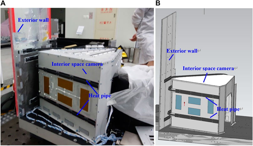
FIGURE 1. Space camera’s installation. (A) Installation of real sample. (B) 3D model assembly.

Therefore, the heat transfer path of the IR camera inside the spacecraft can be simplified as Figure 2. The IR camera is connected to one end of the heat pipe through the thermal interface material, and then, the other end of the heat pipe is connected to the exterior surface of the spacecraft through the thermal interface material.

FIGURE 2

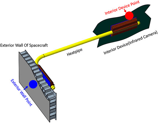
FIGURE 2. The heat transfer path of interior space camera to exterior spacecraft wall.

As shown in Figure 3, there are certain similarities between spacecraft and buildings when performing thermal transient analysis. The designer of a building can evaluate the delay and attenuation of the internal temperature response caused by changes in the temperature or heat flow on the exterior walls (Xing Jin et al., 2012; Lazaros Elias Mavromatidis et al., 2012). The same approach can be used for spacecraft design to evaluate the internal temperature variations caused by heat flow changes on the exterior surface.

FIGURE 3

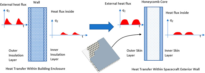
FIGURE 3. Similarities between buildings and spacecraft in the exposure to periodic external heat fluxes.

Transfer Function Analysis Method for Heat Transfer of Space Application

As a rapid and straightforward analytical method, the transfer function method is computationally small and the physical meaning of the analytical results is well defined. Compared with the current mainstream numerical simulation algorithms, it allows the designer to quickly obtain computational results and to enhance the understanding of the physical processes of heat transfer (A.B. Sproul, 2017).

Fourier Transform of Periodic External Heat Flow

For external heat flow with periodic fluctuations, the time-varying external heat flow can be converted into multiple sinusoidal waves with different frequencies and phases using the time-domain and frequency–domain conversion methods commonly used in electronic signal processing (Liao et al., 2021). In engineering practice, periodic functions (whose frequencies are called fundamental waves) can be decomposed into a finite number of sinusoids (called harmonics) with integer multiples of the fundamental waveform.

The concept of the discrete Fourier transform could be introduced and the fast Fourier transform (FFT) algorithm utilized. The external heat flow function could then be decomposed into several sinusoids with different amplitudes, frequencies, and phases. This is shown in Eq. 3.

$q\left(\tau \right)=\overline{q}+{{\displaystyle \sum }}_{n=1}^{\infty }{a}_{n}sin\left(\frac{2\pi n\tau }{T}+{\psi }_n\right)(2)$

where $\overline{q}$ denotes the average value of the external heat flow; $a_n$ denotes the amplitude of the corresponding frequency; $T$ denotes the period of the external heat flow function; and ${\phi }_n$ denotes the phase of the corresponding frequency, respectively.

When using the FFT algorithm for conversion between the time and frequency domains, the external heat flow is first sampled, and the following two restrictions must be considered when sampling.

1) Sampling theorem, also known as Nyquist’s theorem. The sampling frequency must be at least twice as large as the frequency of the signal of interest. For example, if we want to extract and calculate the fifth-order harmonics of the external heat flow for a 24-h conversion period, the fundamental frequency of the external heat flow is $\frac{1}{24\text{h}}$ and the fifth-order harmonic frequency is $\frac{5}{12\text{h}}$, and the sampling frequency used to discretize the continuous external heat flow signal must be greater than $\frac{5}{6\text{h}}$.

2) The quantity of samples required by the FFT algorithm. The FFT uses the parity feature of the data sequence to decompose each computational sequence into even and odd sequences, and then, using the concept of complex real and imaginary parts, the time complexity of the discrete Fourier transform can be reduced from $\text{O}\left({\text{N}}^2\right)$ to $\text{O}\left(\text{N}\log \text{N}\right)$. Therefore, the number of samples must be increased to the power of 2, i.e., $\text{N}=2^{\text{m}}$.

By introducing Euler’s formula ${\text{e}}^{\text{ix}}=\text{cosx}+\text{isinx}$, the trigonometric functions in the Fourier transform can be transformed into complex exponential functions. Figure 4 illustrated the Fourier transform of a periodically varying external heat flow used in this paper later.

$q\left(\tau \right)=\overline{q}+\text{Im}{\displaystyle \sum }_{n=1}^{\infty }{a}_n{e}^{i\left(\frac{2\pi n\tau }{T}+{\psi }_n\right)}(3)$

FIGURE 4

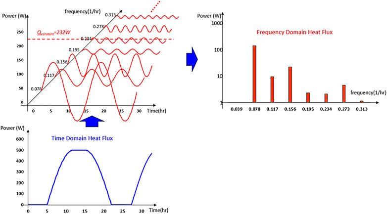
FIGURE 4. Fourier transform from time domain to frequency domain.

Governing Equation

Aforementioned, the exterior wall of the spacecraft consists of three parts, with a honeycomb layer in the middle and thin aluminum skin layers on either side. For each layer of the structure, which can be considered as a thin shell, its heat transfer can also be considered as a one-dimensional heat transfer problem.

The transfer function method is utilized to solve this one-dimensional transient heat transfer problem. The solution is carried out by the set of transient heat transfer partial differential equations shown in Eq. 4.a and Eq. 4.b

$\frac{\partial t\left(x,\tau \right)}{\partial \tau }=\alpha \frac{\partial t^2\left(x,\tau \right)}{\partial x^2}$(4.a)

$q\left(x,\tau \right)=-\lambda \frac{\partial t\left(x,\tau \right)}{\partial x}$(4.b)

where $\alpha$ is the thermal diffusivity which is given by $\alpha =\raisebox{1ex}{$\lambda $}\!\left/ \!\raisebox{-1ex}{$c\rho $}\right.$.

Laplace Transform

The transfer function method is resolved by a mathematical Laplace transformation. Through this method, the partial differential equations are turned into the corresponding algebraic equations. After resolving the algebraic equations, the inverse Laplace transform equations should be used to obtain the corresponding heat flow and temperature values.

$L\left[t\left(x,\tau \right)\right]\tau =\underset{0}{\overset{\infty }{{\displaystyle \int }}}t\left(x,\tau \right)e^{-s}d\tau =T\left(x,s\right)$(5.a)

$L\left[q\left(x,\tau \right)\right]\tau =\underset{0}{\overset{\infty }{{\displaystyle \int }}}q\left(x,\tau \right)e^{-s\tau }d\tau =Q\left(x,s\right)$(5.b)

Transfer Function Matrix

The transfer function matrices of each layer structure for heat flow and temperature are finally obtained by solving the Laplace transform of the governing equation (Eq. 6).

$\left[G\right]=\left[\begin{array}{cc}A\left(s\right)& -B\left(s\right)\\ -C\left(s\right)& D\left(s\right)\end{array}\right]=\left[\begin{array}{cc}ch\left(\sqrt{\frac{s}{\alpha }}x\right)& -sh\left(\sqrt{\frac{s}{\alpha }}x\right)/\lambda \sqrt{\frac{s}{\alpha }}\\ -\lambda \sqrt{\frac{s}{\alpha }}sh\left(\sqrt{\frac{s}{\alpha }}x\right)& ch\left(\sqrt{\frac{s}{\alpha }}x\right)\end{array}\right](6)$

Utilizing the transfer function matrix, once the Laplace transform values of the temperature and heat flow on one side of the thin-walled structure are known, the Laplace transform values of the temperature and heat flow on the other side of the thin-walled structure can be solved.

$\left[\begin{array}{c}T\left(i,s\right)\\ Q\left(i,s\right)\end{array}\right]=\left[G\right]\left[\begin{array}{c}T\left(o,s\right)\\ Q\left(o,s\right)\end{array}\right](7)$

where $\text{T}\left(\text{i},\text{s}\right)$ and $\text{Q}\left(\text{i},\text{s}\right)$ denote the Laplace transform values of the temperature and heat flow inside the thin-walled structure, respectively, and $\text{T}\left(\text{o},\text{s}\right)$ and $\text{Q}\left(\text{o},\text{s}\right)$ denote the Laplace transform values of the temperature and heat flow outside the thin-walled structure, respectively.

Considering that the object under analysis possesses a three-layer structure, the overall transfer function matrix of the exterior surface of the spacecraft from the outside to the inside is

$\left[\text{G}\right]=\left[{\text{G}}_1\right]\left[{\text{G}}_2\right]\left[{\text{G}}_3\right](8)$

where $\left[{\text{G}}_1\right]$ denotes the heat transfer function matrix of the exterior aluminum skin, $\left[{\text{G}}_2\right]$ denotes the heat transfer function matrix of the honeycomb panel core plate, and $\left[{\text{G}}_3\right]$ denotes the heat transfer function matrix of the interior aluminum skin.

Heat pipes and thermal interface materials can be considered as purely thermally resistive devices, and they have a limited and negligible heat capacity; therefore, their transfer function matrices are as follows (Jie Zhu et al., 2010; Ádám Bácsi, 2019):

$\left[G\right]=\left[\begin{array}{cc}1& R\\ 0& 1\end{array}\right](9)$

where $R$ denotes the thermal resistance of the heat pipe or thermal interface material.

The matrix of transfer functions on the whole heat transfer path is illustrated in Figure 5.

FIGURE 5

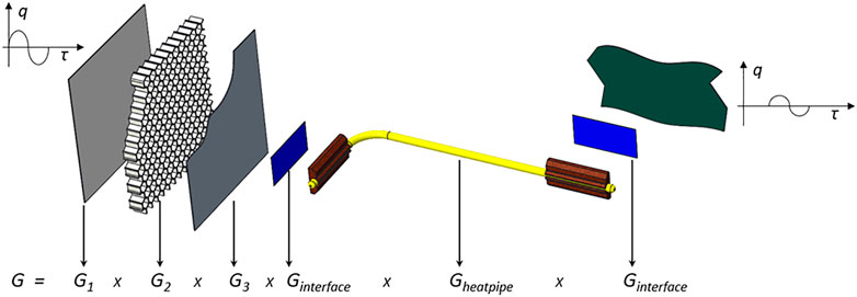
FIGURE 5. Transfer function matrix along the heat transfer path.

After solving the governing equations and obtaining the Laplace domain solutions for temperature and heat flow, the inverse Laplace transform can be used to obtain the solutions for temperature and heat flow.

In the heat transfer process, there is a certain lag in the heat transfer process due to the existence of the heat capacity of the shell itself. The time delay from the peak time of the exterior surface temperature waveform to the peak of the interior surface temperature waveform can be defined as ξ, expressed as Eq 10.

$\xi =t_{i,max}-t_{o,max}(10)$

Aforementioned, the temperature response of the equipment inside the spacecraft to external heat flow has limited relevance to radiation and depends mainly on the time required for heat transfer to reach equilibrium along the conduction path.

Temperature disturbances of different frequencies are applied to the exterior surfaces of the spacecraft walls. The temperature response delay time of the equipment inside the spacecraft can be determined by solving the transfer function matrix and the correlation equation.

Case Studies

The thermophysical parameters along the heat dissipation path of the IR camera device as the object of research are presented in Table 1.

TABLE 1

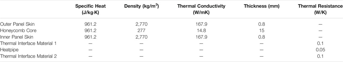
TABLE 1. Thermal properties of different material through the heat transfer path.

Time Delay Analysis

The time lag of temperature response calculated are shown as Figure 6.

FIGURE 6

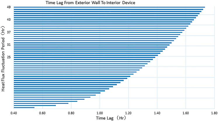
FIGURE 6. Time lag from exterior wall to interior device of different heat flux fluctuation.

The commercial software TMG is utilized for transient thermal simulation to obtain the temperature response of the internal device when the external heat flow varies periodically. By observing the delay in the peak time of the internal device temperature response relative to the peak time of the wall temperature, it is feasible to compare the consistency of the delay values of the different methods. Figure 7 shows the temperature change from the exterior surface of the spacecraft to the interior device and its time delay under external heat flow with different frequencies of sinusoidal waves. The results simulated by commercial software are compared with the calculated values of the methods described in this paper.

FIGURE 7

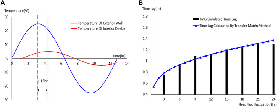
FIGURE 7. Time lag comparison between transfer function method and TMG simulation. (A) Time lag for fluctuations with a period of 12.8 hrs. (B) Time lag caused by fluctuations at different cycles.

As shown in Figure 7, the time lag from the exterior wall to the interior unit calculated by the transfer function method used in this paper is consistent with the results obtained from the TMG software simulation. This also proves that the method used in this paper is reliable in calculating the time response, although it does not require a detailed model.

Figure 7A illustrates the time lag between the exterior wall and the interior equipment for a heat flux with 12.8-h cycle fluctuations. Figure 7B shows a comparison of the time lags calculated with the TMG tool and the transfer matrix method.

Attenuation Calculation

When the external heat flow varies, the temperature of the outer surface of the spacecraft varies first, and, after a certain time lag, the temperature of the interior devices also varies. The parameter of most concern when assessing the effect of external heat flow fluctuations is the magnitude of the interior device temperature variation.

On the basis of the aforesaid analysis and calculation of the time delay, it can be observed that the time delay is basically within 2 h. Therefore, if the variation period of external heat flow is more than 12 h, then the transient heat transfer can be considered as several steady processes. See Figure 8.

FIGURE 8

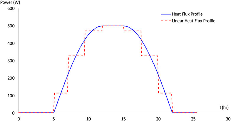
FIGURE 8. Linearization of periodic external heat flux.

After linearizing the external heat flux, as illustrated in Figure 8, it is possible to calculate the value of the temperature variation of the exterior walls of the spacecraft and the interior equipment for different power levels of external heat flux.

For the convenience of the analysis, $\text{θ}$ is defined as the temperature rise due to a certain level of heat flux. In addition, the attenuation ratio of the temperature change of the internal device to the magnitude of the temperature change outside the spacecraft can be defined, as shown in Eq. 11.a and Eq. 11.b.

$\theta =t_{max}-t_{initial}$(11.a)

$f=\frac{{\theta }_{interior device}}{{\theta }_{exterior wall}}$(11.b)

Figure 9 demonstrates a schematic of the thermal path from the exterior wall of the spacecraft to the interior IR camera.

FIGURE 9

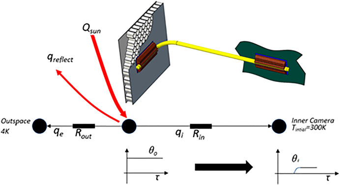
FIGURE 9. Schematic diagram of the thermal transfer path.

Commercial software TMG was used to solve the temperature changes of the exterior wall and the inner IR camera after reaching a steady state under various external heat flux densities.

Figure 10 illustrates the spacecraft temperature distribution simulated by TMG when the external heat flux is 500 W per square meter, where the blue dots represent the temperature monitoring point of the exterior wall of the spacecraft, and the red dots represent the interior device monitoring point of the IR camera.

FIGURE 10

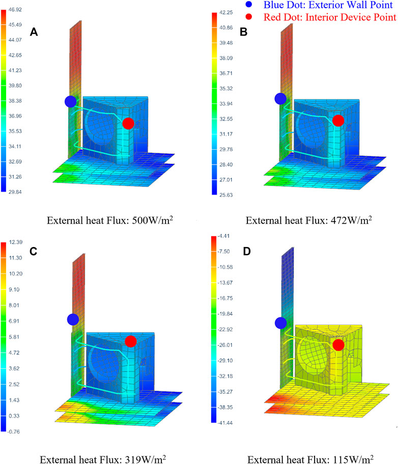
FIGURE 10. Temperature contours of the interior device under different external heat flux. A-D show the temperatures at different heat fluxes.

Table 2 shows a summary of the simulation results. The attenuation rates of the temperature rise at the two monitoring points at different external heat fluxes are presented here.

TABLE 2

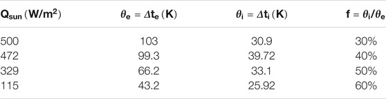
TABLE 2. Attenuation ratio when different heat flux applied.

Experiment Validation

Figure 11 illustrates the test environment setup. The test results were obtained by monitoring the temperature of one monitoring point on the exterior wall of the spacecraft and another monitoring point on the interior unit of the IR camera (see Figure 12). It can be seen that the time lag between these two monitoring points when an external heat flux is applied is consistent with the values archived from the transfer function method and the simulation results of TMG. In addition, the temperature variations of the exterior wall monitor and the interior equipment monitor are in agreement with the simulation results of TMG.

FIGURE 11

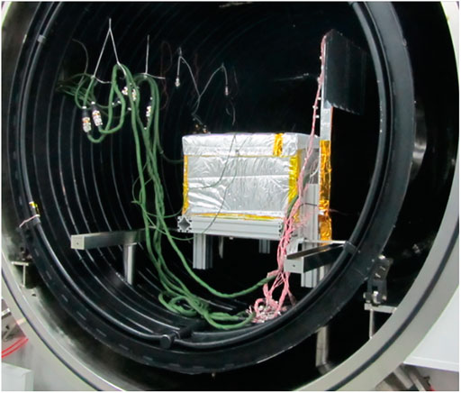
FIGURE 11. Experiment setup.

FIGURE 12

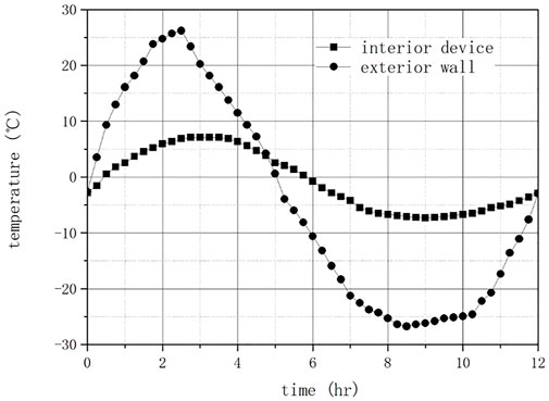
FIGURE 12. Temperature profile of two monitor points under different heat flux.

Conclusion

In this paper, the concept of transfer function is innovatively applied to thermal control design and provides a unique perspective for designers. The solution process and results have a clear physical meaning. This not only enables the thermal designer to clearly communicate the design concept and its results to other designers but also provides clear access to the influence of the parameters of each part of the product in the heat transfer process, which is crucial in subsequent optimization.

The calculation method used in this paper is reliable compared to conventional commercial software and experimental results. As an analytical method for numerical heat transfer, it is computationally small and, therefore, suitable for embedding the algorithm in the control unit of the on-board equipment to actively predict the effect on the internal devices when the external heat flow changes.

Meanwhile, it must also be emphasized by the authors that the analytical method only considers the influence of limited parameters and its accuracy cannot be compared with the mainstream numerical simulations, the limitations of which is obvious; firstly, the heat transfer path must be simple and, also, the results need to be compared with those of certain numerical simulations before the approach can be safely applied to product design.

In product design, there will certainly be numerous situations and cases where the application of transfer functions is applicable. How these applications can be specifically carried out, how they can be verified in later simulations and experiments, how they can be applied to deliver shorter product development cycles and lower development costs, and how they can be integrated with other optimization methods and thermal control algorithms to bring about performance improvements are all topics that can be studied in the next work.

Data Availability Statement

The raw data supporting the conclusion of this article will be made available by the authors, without undue reservation.

Author Contributions

JQ performed the data analyses and wrote the manuscript. LS provided corresponding technical support and advice on writing the paper. All authors contributed to the article and approved the submitted version.

Funding

The work was supported by the Youth Innovation Promotion Association of the Chinese Academy of Sciences (2018273) and the National Key R&D Program of China (2016YFB0500601).

Conflict of Interest

The authors declare that the research was conducted in the absence of any commercial or financial relationships that could be construed as a potential conflict of interest.

Publisher’s Note

All claims expressed in this article are solely those of the authors and do not necessarily represent those of their affiliated organizations or those of the publisher, the editors, and the reviewers. Any product that may be evaluated in this article, or claim that may be made by its manufacturer, is not guaranteed or endorsed by the publisher.

Supplementary Material

The Supplementary Material for this article can be found online at: https://www.frontiersin.org/articles/10.3389/fenrg.2022.833071/full#supplementary-material

References

Bácsi, Á. (2019). The Number of Independent Elements in Heat Transmission Matrices. Int. J. Therm. Sci. 138, 496–503. doi:10.1016/j.ijthermalsci.2019.01.005

CrossRef Full Text | Google Scholar

Batsale, M. J.-C., Jean-Christophe Batsale, J., and Morikawa, J. (2020). Quadrupole Modelling of Dual Lock-In Method for the Simultaneous Measurements of thermal Diffusivity and thermal Effusivity. Int. J. Heat Mass Transfer 162, 120337. doi:10.1016/j.ijheatmasstransfer.2020.120337

CrossRef Full Text | Google Scholar

Davidson, J. N., Stone, D. A., and Foster, M. P. (2014). Required Cauer Network Order for Modelling of thermal Transfer Impedance. Electron. Lett. 50 (4), 260–262. doi:10.1049/el.2013.3426

CrossRef Full Text | Google Scholar

Derakhtenjani, A. S., and Athienitis, A. K. (2021). A Frequency Domain Transfer Function Methodology for thermal Characterization and Design for Energy Flexibility of Zones with Radiant Systems. Renew. Energ. 163, 1033–1045. doi:10.1016/j.ijheatmasstransfer.2020.120600

CrossRef Full Text | Google Scholar

El Maakoul, A., Degiovanni, A., and Bouhssine, Z. (2020). Transient Linear Analytical Heat Transfer Model for a Building, Validation with a Non-linear Coupled Finite Volume Code. Therm. Sci. Eng. Prog. 20, 100756. doi:10.1016/j.tsep.2020.100756

CrossRef Full Text | Google Scholar

Evola, G., and Marletta, L. (2013). A Dynamic Parameter to Describe the thermal Response of Buildings to Radiant Heat Gains. Energy and Buildings 65, 448–457. doi:10.1016/j.enbuild.2013.06.026

CrossRef Full Text | Google Scholar

Ginestet, S., Bouache, T., Limam, K., and Lindner, G. (2013). Thermal Identification of Building Multilayer walls Using Reflective Newton Algorithm Applied to Quadrupole Modelling. Energy and Buildings 60, 139–145. doi:10.1016/j.enbuild.2013.01.011

CrossRef Full Text | Google Scholar

Janicki, M., Torzewicz, T., and Napieralski, Z. K. A. (20212013). Accuracy and Boundary Condition independence of Cauer RC Ladder Compact thermal Models. Microelectronics J. 44 (Issue 7), 619–622. doi:10.1016/j.mejo.2013.02.020

CrossRef Full Text | Google Scholar

Jin, X., Zhang, X., Cao, Y., and Wang, G. (2012). Thermal Performance Evaluation of the wall Using Heat Flux Time Lag and Decrement Factor. Energy and Buildings 47, 369–374. doi:10.1016/j.enbuild.2011.12.010

CrossRef Full Text | Google Scholar

Koutsakis, G., Nellis, G. F., and Ghandhi, J. B. (2020). Surface Temperature of a Multi-Layer thermal Barrier Coated wall Subject to an Unsteady Heat Flux. Int. J. Heat Mass Transfer 155, 119645. doi:10.1016/j.ijheatmasstransfer.2020.119645

CrossRef Full Text | Google Scholar

Liao, L., Zhang, C., and Gang, W. (2021). Frequency thermal Characteristic and Parametric Study of Multi-Functional Building Envelope for Coolth Recovery and thermal Insulation: Modelling and Experimental Validation. Energy & Buildings 253, 1115412. doi:10.1016/j.enbuild.2021.111541

CrossRef Full Text | Google Scholar

Mavromatidis, L. E., El Mankibi, M., Michel, P., and Santamouris, M. (2012). Numerical Estimation of Time Lags and Decrement Factors for wall Complexes Including Multilayer Thermal Insulation, in Two Different Climatic Zones. Appl. Energ. 92, 480–491. doi:10.1016/j.apenergy.2011.10.007

CrossRef Full Text | Google Scholar

Miao, Y., Huang, C., Yu, L., Lv, L., Qiao, L., and Wang, X. (2020). Study on the Calculation of Unsteady Radiant Heat Transfer Load with Stratified Air Distribution Based on Harmonic Reaction Method. Energy and Buildings 226, 110401. doi:10.1016/j.enbuild.2020.110401

CrossRef Full Text | Google Scholar

Pailhes, J., Pradere, C., Battaglia, J.-L., Toutain, J., Kusiak, A., Aregba, A. W., et al. (2012). Thermal Quadrupole Method with Internal Heat Sources. Int. J. Therm. Sci. 53, 49–55. doi:10.1016/j.ijthermalsci.2011.10.005

CrossRef Full Text | Google Scholar

Sproul, A. B. (2017). Admittance/Fourier Series Revisited: Understanding Periodic Heat Flows. Proced. Eng. 180, 292–302. doi:10.1016/j.proeng.2017.04.188

CrossRef Full Text | Google Scholar

Thomas, L. P., Marino, B. M., and Muñoz, N. (2020). Steady-state and Time-dependent Heat Fluxes through Building Envelope walls: A Quantitative Analysis to Determine Their Relative Significance All Year Round. J. Building Eng. 29, 101122. doi:10.1016/j.jobe.2019.101122

CrossRef Full Text | Google Scholar

Wang, J., Wang, S., Xu, X., and Chen, Y. (2009). Short Time Step Heat Flow Calculation of Building Constructions Based on Frequency-Domain Regression Method. Int. J. Therm. Sci. 48, 2355–2364. doi:10.1016/j.ijthermalsci.2009.05.005

CrossRef Full Text | Google Scholar

Yumrutaş, R., Ünsalb, M., and Kanoğlu, M. (2005). Periodic Solution of Transient Heat Flow through Multilayer walls and Flat Roofs by Complex Finite Fourier Transform Technique. Building Environ. 40, 1117–1121. doi:10.1016/j.buildenv.2004.09.005

CrossRef Full Text | Google Scholar

Zhu, J., Tang, D., Wang, W., Liu, J., Holub, K. W., and Yang, R. (2010). Ultrafast Thermoreflectance Techniques for Measuring thermal Conductivity and Interface thermal Conductance of Thin Films. J. Appl. Phys. 108, 094315. doi:10.1063/1.3504213

CrossRef Full Text | Google Scholar