IGV Optimization for a Large Axial Flow Fan Based on MRGP Model and Sobol’ Method

Large axial flow fans with inlet guide vanes (IGVs) have been widely used in building ventilation systems. However, it does not readily satisfy the increasing demand for energy saving, high efficiency, or noise reduction. The rotor-stator interaction between the IGVs and the impeller is particularly important for the aerodynamic performance and noise of the fans. Therefore, this article takes a large axial fan, combined with parameterization methods to optimize the IGVs. Based on numerical simulation analysis, the multiple-response Gaussian process (MRGP) approximate model was established to optimize the IGVs structure, and the Sobol´ method was employed for sensitivity analysis. The best model was selected for proofing analysis, and the experimental and numerical simulation results show that the total pressure of the optimized fan increased by 144.4 Pa and the noise decreased by 7.2 dB. These results verify that the multi-objective optimization design method combining the MRGP approximate model and the Sobol´ method demonstrates high credibility and provides a key design direction for the design optimization of large axial flow fans. This novel optimization method also has easy-to-understand parameters and the coupling relationships between parameters and responses, which has potential value for the design of other types of fluid machinery and provides new ideas for the optimization of fluid machinery.

Introduction

The performance of the ventilation systems is a key concern because its aerodynamic performance and acoustic characteristics are closely related to the user experience (Liu et al., 2013). Large-scale axial flow fans are the main working components of building ventilation systems, and their characteristic parameters determine the overall system’s performance (Kim and Oh, 2018; Carassale et al., 2020).

The three-dimensional flow inside the fan essentially comprises an extremely complex, unsteady, three-dimensional viscous flow (Imtiaz et al., 2018), wherein the interference of the rotor and motion between multi-level rows of blades contribute to periodic unsteadiness inside the fan (Zhou et al., 2018). There are two main interference factors between blade rows: One is caused by the potential flow field in the fan channel, and the other is caused by the wake of the upstream blade row entering the downstream blade row (Thongsri and Pimsarn, 2015; Wang et al., 2015; Hayat et al., 2018). Therefore, understanding the problem of interference between blades and exploring the internal interference mechanisms are crucial for improving the performance of fluid machinery and reducing operating noise.

An axial fan is one of the most used fluid machineries. And most of the research related to fluid machinery focuses on the adjustable blades (Li et al., 2007) and the rotor tip area (Zhang et al., 2019). Varade et al. (Varade et al., 2015) used a three-dimensional Navier-Stokes equations simulation method to study the effects of swept and leaned blades on the fan flow field. Pogorelov et al. (Pogorelov et al., 2016) studied the influence of blade tip gap width on the flow field based on large eddy simulation, and reduced blade tip gap width would enhance the flow of tip gap vortex, thus reducing fan noise. Jung et al. (Jung et al., 2013) studied the impacts of five leading-edge sweep angles on the aerodynamic performance of centrifugal compressors, and they observed that the pressure ratio and efficiency were enhanced to a certain extent at low sweep angles. But at this time, the centrifugal compressors were in uneven flow distribution and poor airflow diffusion efficiency. Therefore, not only the pressure ratio and efficiency of the fan but also the internal flow should be paid attention to. Scholars have carried out multi-objective optimizations considering the strong nonlinearity and discrete variables involved in fluid machinery optimization. The proposed optimization models and methods are universal for fluid machinery designs (Hassan and Crossley, 2015; Li et al., 2017; Liu et al., 2017). Quin D et al. (Quin et al., 2004) explored the influence of different Reynolds numbers on the internal flow characteristics of axial flow fans through the combination of numerical simulation and experimental verification. The installation angle of blades and speed were optimized, and the fan efficiency was improved by 2.4%. Based on the Hicks-Henne equation, Huaxin Zhou et al. (Zhou et al., 2020) designed the optimal route for implementing multi-blade centrifugal fan blades, optimized the blade inlet and outlet installation angles, and improved the air volume and efficiency of the fan. Tolga Baklacioglua et al. (Baklacioglu et al., 2015) modified the algorithm parameters based on the characteristics of algorithms and applied this method to the field of turboprop engines.

Research regarding large-scale axial flow fans considers design standards for high efficiency, high pressure, and low noise. It considers the inlet flow a decisive factor affecting the fan’s efficiency. The (inlet guide vanes) IGVs are used as the guide part of the inlet to deflect the airflow in front of the fan impeller, and its unreasonable design has a great impact on the performance of the fan system. A suitable guide vane structure can reduce dynamic and static interferences, the angle of attack loss, and aerodynamic noise (Burgos et al., 2009; Hyuk and Won-Gu, 2019).

Numerous scholars have investigated blade optimization through approximate models. However, this method has certain limitations. It cannot show the coupling relationships between parameters and responses for practical engineering issues. The present study involved the parametric design of an axial flow fan’s IGVs considering the total pressure and noise as the optimization objectives; the multiple-response Gaussian process (MRGP) approximate model was established to optimize the parameters of the IGVs, and a global sensitivity analysis method based on variance—Sobol ' method was used to clarify the influence of each parameter on the optimization objectives. Finally, numerical simulations and proofing were used to verify and analyze the changes in the flow field characteristics before and after the improvement, while exploring changes in the acoustic characteristics. The proposed multi-objective optimization design method combining an MRGP approximate model and Sobol ' method is universal and adapts to the design optimization of similar machinery.

Research Object

This research focused on the structure of a large axial flow fan, as shown in Figure 2A. The structure is mainly composed of casing, Inlet Guide Vanes (IGVs), moving blades (the only work component), Outlet Guide Vanes (OGVs), cowl, motor, and diffuser tube. The structural parameters are as follows: impeller diameter, D = 1,250 mm; number of moving blades, Z = 14; number of IGVs and OGVs, m₁ = 15, m₂ = 15; rotating speed, n = 1,485 r/min; flow rate, Q = 82400 m³/h at 25°C; total pressure, p_tf = 2,300 Pa; noise, sound pressure level (SPL) = 110.7 dB.

The whole optimization process is shown in Figure 1. Due to CFD calculations and experimental verification, we confirmed that the IGVs are optimization’s objects. The geometric petameters fit the IGVs, then 55 groups of IGVs samples are established. By establishing the MRGP model of relevant optimization variables and the target response, the NSGA-II algorithm was used to solve the model. At the same time, after verifying the feasibility of replacing experiments with numerical simulations, the sample database for the training of MRGP model is calculated by CFD numerical method. After obtaining an optimized IGVs structure, the results were analyzed via proofing verification and numerical simulation analysis. Moreover, Sobol ' method was used to clarify the influence of each parameter on the optimization objectives.

FIGURE 1

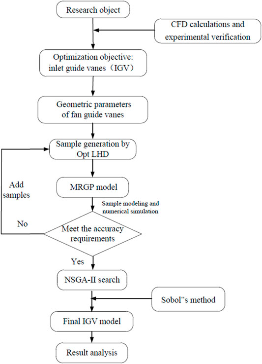
FIGURE 1. Optimization flow chart.

Numerical Simulation Calculation Method and Experimental Verification

The sample database for the MRGP model training is calculated by the CFD numerical method validated by the experiment setup of this paper.

Calculation Model and Meshing

To simplify the geometric model of the fan and extract the internal flow channel area of the fan, the entire axial flow fan was divided into five ducts: the inlet duct, the IGVs duct, the Rotation duct, the OGVs duct, and the outlet duct. Figure 2B shows a simplified diagram of the fan flow domain.

FIGURE 2

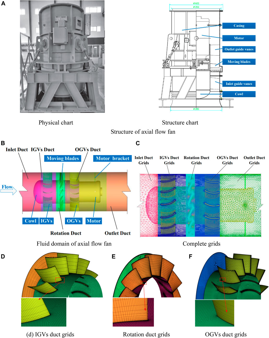
FIGURE 2. Geometric models and meshes. Physical chart Structure chart (A) Structure of axial flow fan (B) Fluid domain of axial flow fan (C) Complete grids (D) IGVs duct grids (E) Rotation duct grids (F) OGVs duct grids.

The complete grids are shown in Figure 2C. The key areas (moving blades, inlet guide vanes, outlet guide vanes) are divided by structured grids to improve the quality of the grid. The grid of the IGVs duct grids, the Rotation duct grids and the OGVs duct grids is shown in Figures 2D–F. Other flow components use unstructured grids. The entire fan grid is shown in Figure 2C. In this case, the first node must be arranged in the area of the viscous bottom layer, with its y⁺ value ≤ 5. The empirical formula for y⁺ is given by Eq. 1 (Moaveni, 1999):

$Y_{\mathrm{w}\mathrm{a}\mathrm{l}\mathrm{l}}=6{\left(\frac{V_{\mathrm{r}\mathrm{e}\mathrm{f}}}{v}\right)}^{-\frac{7}{8}}{\left(\frac{L_{\mathrm{r}\mathrm{e}\mathrm{f}}}{2}\right)}^{\frac{1}{8}}{y}^{+}(1)$

Where Y_wall is the flow field and the thickness of the first layer of the wall, V_ref is the reference speed (m/s), L_ref is the reference length (m), v is the fluid kinematic viscosity (m²/s), and y+ is a dimensionless parameter. According to the empirical formula, the height of the first layer of the boundary layer grid should be < 0.65 mm.

Once the quality of the grids satisfies the requirements, the independence of the computing grids must be verified. As shown in Figure 3, when the total grids number of the fan reaches about 7×10⁶, the total pressure value of the fan obtained by the numerical simulation is generally unchanged, and the total pressure efficiency varies within 1%. Therefore, considering the calculation accuracy and computational time, the number of grids in the entire fan flow domain was 7,230,356.

FIGURE 3

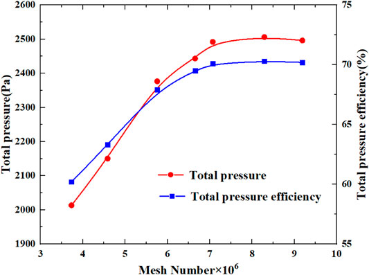
FIGURE 3. Grid independence verification.

Comparative Analysis of Fan Aerodynamic Performance

Air at 25°C was selected as the working fluid, the impeller flow domain was set as the rotation domain, the steady calculation adopted a multiple reference system model (MRF), and the inlet and outlet boundary conditions were set as Mass-flow-inlet and Pressure-outlet. The solution adopted the pressure-based implicit solution, and the standard k-ε turbulence model was used to solve the three-dimensional Reynolds average Navier-Stokes (N-S) equation.

The equation of the standard k-ε turbulence model is as follows:

$\frac{\partial \left(\rho k\right)}{\partial t}+\frac{\partial \left(\rho k{u}_i\right)}{\partial x_i}=\frac{\partial }{\partial x_j}\left[\left(\mu +\frac{{\mu }_i}{{\sigma }_k}\right)\frac{\partial k}{\partial x_i}\right]+G_k-\rho \epsilon (2)$

$\frac{\partial \left(\rho \epsilon \right)}{\partial t}+\frac{\partial \left(\rho \epsilon u_i\right)}{\partial x_j}=\frac{\partial }{\partial x_j}\left[\left(\mu +\frac{{\mu }_i}{{\sigma }_c}\right)\frac{\sigma \epsilon }{\sigma x_j}\right]+\frac{C_{1\epsilon }\epsilon }{k}{G}_k-C_{2\epsilon }\rho \frac{{\epsilon }^{\prime }}{k}(3)$

Where ε is energy loss due to Reynolds stress; σ_k is 1; σ_ε is1.3; C_1ε is 1.44; C_2ε is 1.92; C_μ is 0.09.

Three-dimensional Reynolds-averaged N-S simulations are performed in Fluent to obtain the steady flow field in the test fan, whose governing equations are as follows:

$\frac{\partial \rho }{\partial t}+\frac{\partial \left(\rho u_i\right)}{\partial x_i}=0(4)$

$\frac{\partial \left(\rho u_i\right)}{\partial t}+\frac{\partial }{\partial x_j}\left(\rho u_i{u}_j\right)=-\frac{\partial p}{\partial x_i}+\frac{\partial }{\partial x_j}\left(\mu \frac{\partial u_i}{\partial x_j}-\rho \overline{u_i^{\prime }{u}_j^{\prime }}\right)+S_i(5)$

Where u_i represents the velocity components that are averaged in the x_i direction; ρ, t, μ, and p are the air density, time, dynamic viscosity of the fluid, and average pressure, respectively.

The SIMPLE algorithm was applied to couple the pressure and velocity, and the index parameters of each aerodynamic performance were set to the second-order upwind. The calculation is considered converged when the residual value is less than the convergence residual (1 × 10⁻⁵).

According to the requirements of “GB/T 1236-2017 Standardized Air Duct Performance Experimental for Industrial Ventilators for Air Ducts” (GB/T 1236-2017, 2017), the aerodynamic performance of the large axial flow fan evaluated in this work was tested using a C-type air chamber.

The measured average static pressure differential △p in the pressure relief cylinder at each operating point was obtained. The inlet total pressure is $p_{tf}$, the outlet total pressure is atmospheric pressure P_out, the total pressure of the fan is defined as the difference of total pressure ∆P_b. The flow rate Q and total pressure efficiency ${\eta }_B$ under the standard air condition at each working point were calculated through Eqs., respectively.

$p_{tf}=\frac{\rho }{{\rho }_a}\mathrm{\Delta }p+K\left(\frac{\rho }{2}\right)\times {\left(\frac{Q}{\frac{\pi }{4}\times D_4^2}\right)}^2(6)$

$\mathrm{\Delta }{p}_b=p_{out}-p_{tf}(7)$

$Q=1.111\times \alpha d^2\times \sqrt{\frac{\mathrm{\Delta }p}{{\rho }_a}}(8)$

${\eta }_b=\frac{Q\times \mathrm{\Delta }{p}_b}{P}\times 100\%(9)$

Where $\rho$ is the air density under standard air conditions, ${\rho }_a$ is the air density under test conditions, and $P$ is motor input power, α is flow coefficient.

In the actual measurement, the standard measuring error calculation formula is:

$\sigma =\sqrt{\frac{{\displaystyle \sum {\left(\overline{p}-p_i\right)}^2}}{n-1}}(10)$

Where σ is the standard error values, n is the number of measurements, p_i is the deviation of the measured values from the average, $\overline{p}$ is average values.

Test 10 sets of static pressure data at the design flow Q, as shown in the following Table 1:

TABLE 1

TABLE 1. Static pressure data at the design flow.

Therefore, the standard error values can be calculated by the formula:

$\sigma =\sqrt{\frac{{\displaystyle \sum {\left(\overline{p}-p_i\right)}^2}}{n-1}}=\sqrt{\frac{83.36}{9}}=3.04$

The error analysis of other parameters is the same. According to the standard method, it can be known that the measuring error values are within a reasonable range.

Figure 4A is the schematic diagram of the air performance and field experimental devices. A comprehensive atmospheric pressure, temperature, and air humidity tester was situated at the front end of the inlet collector (air velocity is zero) and used to record the corresponding air parameter values of the axial flow fan under various operating conditions. The performance tests were conducted under normal temperature and pressure. The opening of the cylinder and the flow rate were changed during the experiment by adjusting the intake throttle device. The pressure differences of the Pitot hydrostatic tube and the inlet and outlet pressure were recorded under ten sets of flow conditions.

FIGURE 4

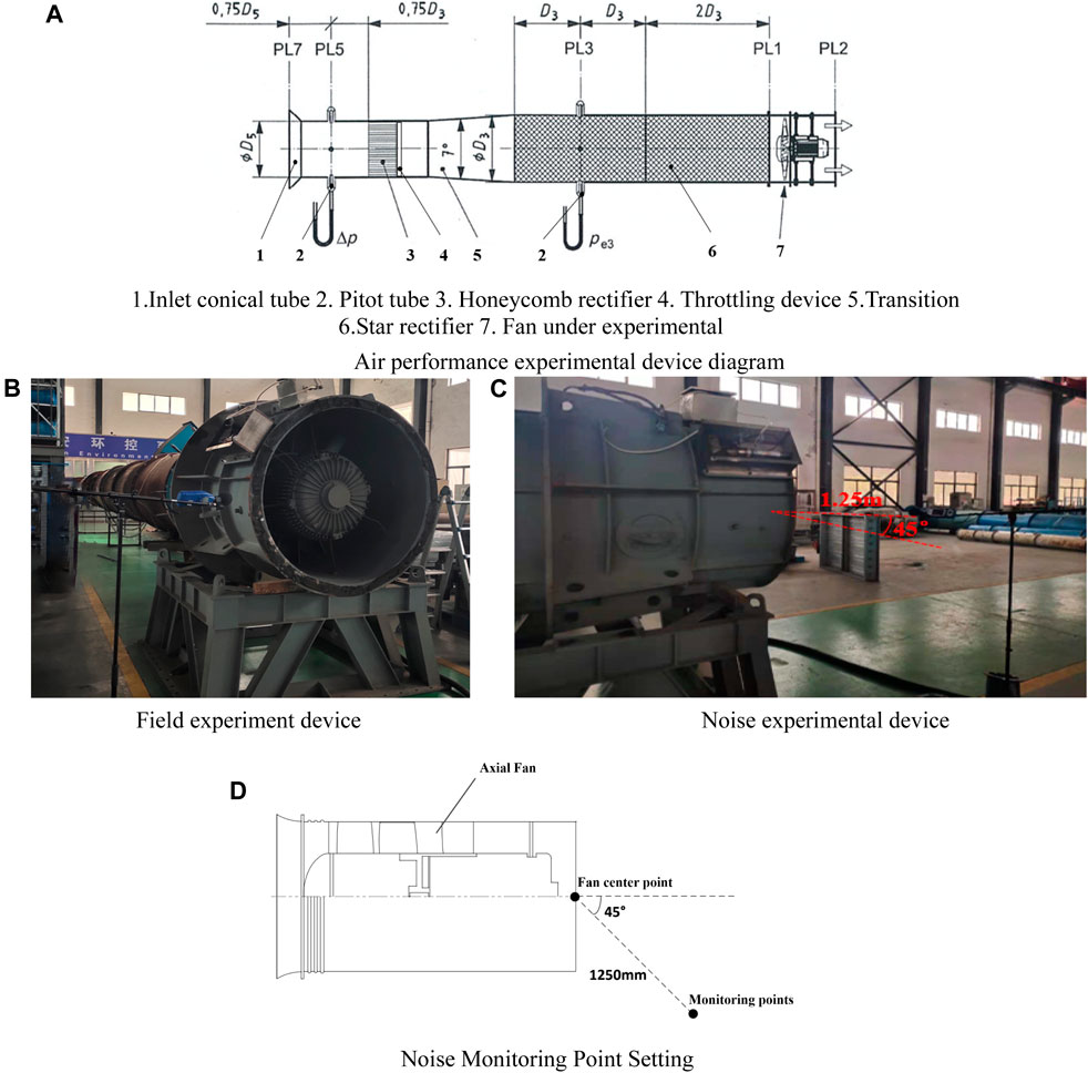
FIGURE 4. Experimental devices. 1. Inlet conical tube 2. Pitot tube 3. Honeycomb rectifier 4. Throttling device 5. Transition 6. Star rectifier 7. Fan under experimental (A) Air performance experimental device diagram (B) Field experiment device (C) Noise experimental device (D) Noise Monitoring Point Setting.

Through CFD calculation, the total pressure $p_{tf}$ (at surface of inlet), $p_{out}$ (at surface of outlet), static pressure $p_i$ (at surface of inlet), flow rate Q (at surface of outlet) and shaft power P₁ of the corresponding position can be directly obtained. Rotating speed, n = 1,485 r/min. The total pressure was calculated by Eq. 7, and the efficiency was calculated by the following equation:

${\eta }_b=\frac{Q\times \mathrm{\Delta }{p}_b}{n\times P_1}\times 100\%(11)$

As shown in Figure 5A, the performance of the original predicted by the numerical simulation was compared with the experimental value. It is clear that the numerical simulation results are well consistent with the experimental values when the flow rate is near the designed flow rate of 80,000–85,000 m³/h. As the flow rate decreases, the pressure simulation value of each operating point is slightly lower than the experimental value, and the maximum error reaches 5%. In contrast, as the flow rate increases, the simulated pressure value at each working point is slightly higher than the experimental value, but the maximum error remains <5%. In contrast, the error between the efficiency experimental and simulated values is small, and the overall error is less than 3%.Therefore, it is considered that the method has high reliability.

FIGURE 5

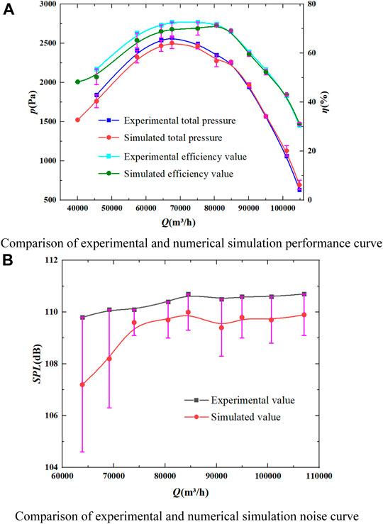
FIGURE 5. Comparison of experimental and simulation results. (A) Comparison of experimental and numerical simulation performance curve (B) Comparison of experimental and numerical simulation noise curve.

Noise Comparative Analysis

Noise simulations adopted the large eddy combined with sound analog theory. The equation of the Ffowcs Williams and Hawkings (FW-H) model (Li et al., 2021) is as follows:

$\frac{1}{c_0^2}\frac{{\partial }^2}{\partial t^2}\left[pH\left(f\right)\right]-{\mathit{\nabla }}^2\left[pH\left(f\right)\right]=\frac{\partial }{\partial t}\left[{\rho }_0{V}_i\frac{\partial f}{\partial x_i}\delta \left(f\right)\right]-\frac{\partial }{\partial x_i}\left[p_{ij}\frac{\partial f}{\partial x_j}\delta \left(f\right)\right]+\frac{{\partial }^2}{\partial x_i\partial x_j}\left[T_{ij}H\left(f\right)\right](12)$

Where c₀ is the sound velocity of the undisturbed fluid, $p$ is the pressure in the fluid, $x_i$ is the space fixed coordinate system, $T_{ij}$ is the fluid viscous stress tensor. And the steady calculation result was used as the initial flow field for the unsteady calculations; the time required for the impeller to rotate 1° is represented by the time step Δt, where Δt = 1/(6n). Therefore, the time step in this study was set to 0.0001 s to obtain near-field flow field information. The commercial software Fluent solves the FW-H equation by calculating the time domain integral and area fraction to determine the fan’s far-field noise. According to the noise test standard “GB/T2888-2008 Fan and Roots Blower Noise Measurement Method” (GB/T2888-2008, 2008), the noise receiving point was set at a horizontal position 45° from the center of the exit surface at a distance equal to the diameter (1,250 mm). Figure 4D presents a schematic diagram showing the setting of noise monitoring points, and Figures 4B,C is a diagram of the experimental device.

The sound field calculation results were obtained via fast Fourier transform to determine each measuring point’s sound pressure level (SPL) and noise spectrum. When CFD calculates the SPL, the time domain solution of the far-field instantaneous sound pressure p' of the FW-H model is first obtained, and then the frequency domain solution is obtained through FFT transformation. The formula for the time domain solution of the instantaneous sound pressure p' can be summarized as (Chen and Zhou, 2021):

$p^{\prime }=\frac{1}{4\pi }{\displaystyle {\int }_{f=0}\left[\frac{L_r}{r^2}\right]}\text{d}S+\frac{1}{4\pi }{\displaystyle {\int }_{f=0}\left[\frac{\stackrel{·}{L_r}}{r^2}\right]}\text{d}S(13)$

In the formula: $L_r=L_i{\widehat{r}}_i$, ${\stackrel{·}{L}}_r={\stackrel{·}{L}}_i{\widehat{r}}_i$, where "." represents the derivative of time, $L_i=p{n}_i$, $n_i$ is the wall normal vector, ${\widehat{r}}_i=\frac{x_i-y_i}{\sqrt{{\left(x_i-y_i\right)}^2}}$, ${\widehat{r}}_i$ represents the unit vector from the sound source to the receiving point, r is the distance from the sound source to the receiving point, c₀ is the speed of sound, taken 340 m/s.

It is clear from Figure 5B that the numerical simulation results are well consistent with the experimental values when the flow rate is above 7,5000 m³/h. As the flow rate decreases, the noise simulation value of each operating point is slightly lower than the experimental value, and the maximum error is less than 3%. When the flow rate is near the designed flow rate, the experiment noise average value was 110.70 dB, the simulated average value was 109.69 dB, and the relative error of the noise value was ≤0.91%.

Guide Vanes Structural Analysis

The fan impeller radial cross-section R = 280 mm (0.5 times blade height) of the flow surface of the blade is selected to study the internal flow characteristics of the fan. Figure 6A shows the schematic diagram of fan impeller radial cross-section.

FIGURE 6

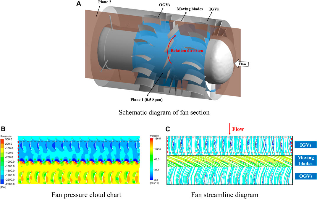
FIGURE 6. Original flow field results. (A) Schematic diagram of fan section (B) Fan pressure cloud chart (C) Fan streamline diagram.

The internal flow field of the original fan was analyzed, and Figure 6B shows the pressure contour of the original fan on plane 1. It is clear from Figure 6B that the negative pressure area of the IGVs of the fan is relatively small, and there is a significant pressure difference in the coupling area between the IGVs and the moving blades, which leads to backflow in the IGVs duct. Figure 6C presents a streamline diagram of the original fan on plane 1, which indicates that the airflow was chaotic before the IGVs optimization, and there was a large amount of backflow in the IGVs duct. Therefore, it can be concluded that the structure has a significant influence on the performance and noise of the fan.

Li J. et al. (Jingyin et al., 2010) found that for an axial flow fan with both inlet and outlet guide vanes, the internal periodic pulsation force is generated by the uneven airflow discharged from the IGVs, which impacts the moving blades. The airflow behind the guide vanes row is uneven because of the wake produced when the airflow through the IGVs, and thus, the absolute velocity of the airflow to the moving blade will change periodically. In addition, Ye Z. (Zengming et al., 2001). determined that the inlet airflow angle and air attack angle relative to the moving blade change periodically. Therefore, the pulsating force of the airflow acting on the moving blade also changes periodically. Because the fan studied in this work has a special structure containing IGVs, the impacts of the IGVs structural parameters on the aerodynamic performance and noise of the fan were analyzed. In addition, Okishi et al. (Okiishi et al., 1970) studied the design of guide vanes profile and found that aerodynamic loss of cascade increases rapidly when the deflector Angle of guide vanes is greater than 35°. Therefore, the pulsating force of the airflow acting on the moving blade also changes periodically. Because the fan studied in this work has a special structure containing IGVs, the impacts of the IGVs structural parameters on the aerodynamic performance and noise of the fan were analyzed.

Selecting the appropriate structural parameters of the IGVs is of great significance for the performance optimization of large-scale axial flow fans. The IGVs is an equal-thickness blade whose shape is formed by thickening the midline of the tip and root of the blade; thus, the blade shape is related to the tip and root deflection angles. Accordingly, the guide vanes tip deflection angle (θ_a) and root deflection angle (θ_b) were selected as two optimization variables.

The blade installation angle reflects the axial installation position of the blade relative to the hub, and it is an important structural factor that affects the operating performance of the fan (Okiishi et al., 1970). As the blade installation angle becomes smaller, the pressure side of the fan blades increases, and the blade load increases accordingly. Moreover, the operating noise of the fan will increase. Extreme blade installation angles may also reduce the performance of the fan. When the blade installation angle is too small, although the load on the blade decreases, the pressure, flow rate, and efficiency of the fan will be reduced. Therefore, the installation angle of the leading vane was selected as one of the optimization variables. As shown in Figure 7, the installation angle of the IGVs is defined as θ_a.

FIGURE 7

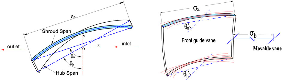
FIGURE 7. Geometric parameters of fan guide vanes.

For axial fans with IGVs, the installation position of the IGVs has a significant impact on the performance and noise of the fan. Considering the mechanism of rotating noise generation, the vortex created by the irregular flow of the IGVs and the airflow at the tip of the moving blade was used to establish a vortex model (Rufu and Hongwu, 1998). The mathematical expression of the relationship between wake performance and the axial distance between the IGVs and the moving blades, Eq. 14 (Dittmar, 1972).

$\frac{V^{\prime }}{V_0}=\frac{1.6\sqrt{C_D}}{{\left({\sigma }_b/{\sigma }_{\text{a}}\right)}^{1/2}}(14)$

Where $V^{\prime }$ is maximum difference from free stream velocity in the wake, length/time (m/s), V₀ is free-stream velocity at upstream blade-row inlet, length/time (m/s), C_D is profile drag coefficient is a constant (determined by leaf shape), σ_b is the distance between moving blades and guide vanes, σ_a is guide vane chord length.

Eq. 14 indicates that as the axial distance σ_b of the guide vanes increases, the vortex velocity decreases, thereby reducing the lift pulsation and noise generated by the irregular flow through the IGVs and ultimately impacting the rotor. Theoretically, increasing the axial distance can weaken the interaction between the moving blade and the IGVs, thus reducing the noise.

The parameters of the guide vanes of the large axial flow fans is: σ_a = 292 mm, σ_b = 260 mm, θ_a = 72°, θ_b = 62°.

Sensitivity Analysis of Combined MRGP and Sobol´’s Method

The chord length of the leading blade σ_a, the axial distance σ_b from the IGVs to the moving blades, the tip deflection angle of the guide vanes θ_a, and the root deflection angle of the guide vanes θ_b were used as input variables, and the total pressure and noise value of the fan were the output values used to establish a multi-dimensional respond to the Gaussian proxy model. Meanwhile, Sobol'’s method was used for the sensitivity analysis of the variables. In this way, an active learning sensitivity method based on the combined MRGP and Sobol' method was established for large-scale axial flow fans.

The MRGP model is an extension of the Kriging model because the traditional Kriging model could only deal with problems involving multivariate single response output. Multiple Kriging models must be constructed; however, this approach does not account for the coupling-related issues affecting the response values. Therefore, the MRGP model for multi-variable and multi-response problems has gradually attracted attention.

Zhen et al. (2017) was the first to propose the MRGP model, which combines m functions into a concrete realization of a multi-response Gaussian process (Dittmar, 1972).

$G\left(x\right)=f{\left(x\right)}^{\text{T}}B+Z\left(x\right)(15)$

Among them, the polynomial regression function f(x) is the same as the Kriging model, but the regression coefficient B is an n×m matrix, and Z(x) is expanded to a 1×m row vector. The covariance of Z(x) is represented by an m×m covariance matrix, i.e., Σ^m.

${\displaystyle {\sum }^m}=\left[\begin{array}{ccc}{\sigma }^2\left(g_1,g_2\right)& \cdots & {\sigma }^2\left(g_1,g_m\right)\\ ⋮& \ddots & ⋮\\ {\sigma }^2\left(g_m,g_1\right)& \cdots & {\sigma }^2\left(g_m,g_m\right)\end{array}\right](16)$

The specific principle governing the association of the two responses is shown in Figure 8 below.

FIGURE 8

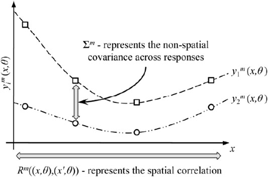
FIGURE 8. Schematic diagram of MRGP model.

FIGURE 9

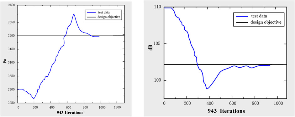
FIGURE 9. Matlab global optimization.

In the present work, the MRGP model was selected as the approximate function, and 55 sets of variables and corresponding response sample datapoint (obtained by Opt LHD combined with numerical simulations) were used to establish an approximate model. The first 50 sets were used as sample matrix data, and the last five sets were used as test data.

Selecting the range of 20% fluctuation of the original parameters as the variable range, and the variation range of the design variable parameters is: σ_a = 233.6∼350.4mm, σ_b = 208∼312mm, θ_a = 57.6∼86.4°, θ_b = 49.6∼74.4°.

The limitations of parameter selection led to certain errors in the constructed MRGP model. Therefore, to verify the accuracy of the model, it must be tested with the relevant experimental accuracy formula before the prediction is solved. This study applied global sensitivity analysis based on Sobol ' method, which is a Monte Carlo method based on analysis of variance. Sobol ' method uses the total variance D to indicate the degree of influence of all parameters on the model results, which can be expressed as shown in Eq. 17:

$D={\displaystyle \int f^2\left(x\right)}\text{d}x-f_0^2(17)$

The partial variance D_i is used to indicate the degree of influence of a single parameter or the effect of the parameters on the model result, this term is expressed by Eq. 18:

$D_{i_1,i_2,\cdots ,i_t}={\displaystyle \int f_{i_1,i_2,\cdots ,i_3}^2}\text{d}{x}_{i_1}\text{d}{x}_{i_2}\cdots \text{d}{x}_{i_s}(18)$

The Sobol´ method is used to evaluate the sensitivity of the approximate function obtained by MRGP by solving the first-order and overall global sensitivity parameters of each influencing factor. The first-order sensitivity indicates the degree of influence of a single factor on the total pressure and noise of the fan. The overall sensitivity indicates the degree of influence of a single factor on the total pressure and noise of the fan and reflects the interactions with other influencing factors. Therefore, when the first-order sensitivity of a variable differs significantly from the overall sensitivity, it can be concluded that factor has a significant interaction (Table 2).

TABLE 2

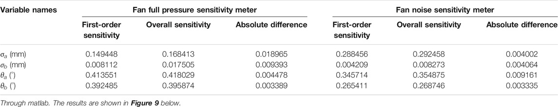
TABLE 2. Fan sensitivity meter.

Table 3 shows the structural parameters corresponding to the optimal solution and the total pressure and noise at the design operating point. It is clear that at the design operating point, the total pressure of the fan has increased by 126.86 Pa, and the noise has dropped by 6.85 dB.

TABLE 3

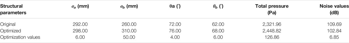
TABLE 3. Structural parameters corresponding to the optimal solution.

Results Analysis

Figure 10A shows the optimized the IGVs shapes. Comparing the optimized geometries of the inlet and outlet vanes revealed that the chord length of the IGVs σ_a was increased by 6 mm, the axial distance from the IGVs to the moving blades σ_b was increased by 50 mm, and the tip deflection angle θ_a of the IGVs was increased by 4°, while the root deflection angle θ_b increased by 6°. Figure 10 confirms the optimization of the fan (Original vs Optimized).

FIGURE 10

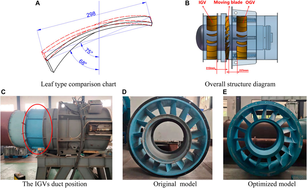
FIGURE 10. The proofing model Original and Optimized. (A) Leaf type comparison chart (B) Overall structure diagram (C) The IGVs duct position (D) Original model (E) Optimized model.

Analysis of Test Results

The optimization significantly improved the aerodynamic performance of the fan. The optimized fan was sampled to facilitate the analysis of the original versus optimized results, and its aerodynamic performance was analyzed experimentally. Figure 11 shows the fan performance curves before and after optimization. The performance curve of the optimized fan was consistent with the original fan’s performance curve; The optimized fan’s total pressure and total pressure efficiency under various operating conditions were improved. Specifically, at the design operating point, the fan’s total pressure increased by approximately 144.4 Pa. The efficiency of the fan improved at low flow, and was essentially unchanged at the design operating point.

FIGURE 11

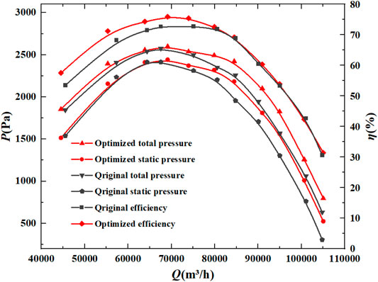
FIGURE 11. Fan performance curves original and optimized.

Table 4 shows the noise values of the original and optimized IGVs structures under various working conditions, revealing that the fan noise was significantly reduced after optimization. Under low flow conditions, the SPL was only reduced by 6.5 dB. As the flow rate increased, the optimized fan’s SPL could be reduced by 7.2 dB, and when the air volume exceeded 70000 m³/h, the SPL changed only slightly with the air volume. At the design operating point, the fan’s SPL was reduced by 7.2 dB (from 110.4 to 103.2 dB), which was a clear noise reduction effect.

TABLE 4

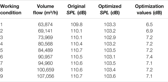
TABLE 4. Experimental the noise value under each working condition.

To accurately analyze the noise, a B&K microphone was used to obtain the noise spectrum; Figure 12A shows the B&K experimental equipment. According to the noise test standard “GB/T2888-2008 Fan and Roots Blower Noise Measurement Method”, the B&K microphone was arranged at a horizontal position at 45° from the center of the outlet surface at a distance equal to the diameter (1250 mm) (GB/T2888-2008, 2008). The experimental device is shown in Figure 12B.

FIGURE 12

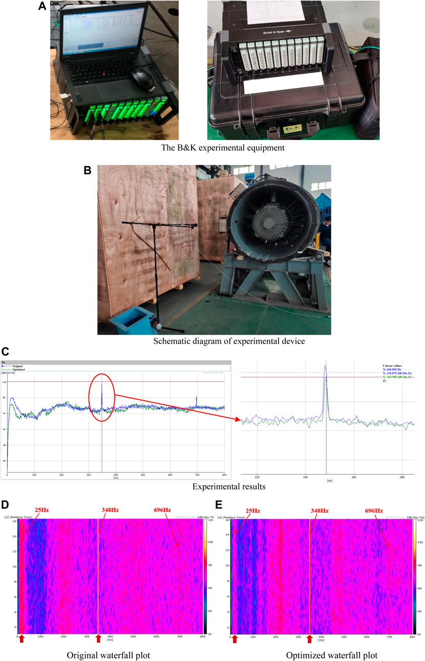
FIGURE 12. Noise experimental results. (A) The B&K experimental equipment (B) Schematic diagram of experimental device (C) Experimental results (D) Original waterfall plot (E) Optimized waterfall plot.

The test results indicate that the original and optimized SPL spectral distributions reached their peaks at the fundamental frequency and its multiples. This is because over the tested frequency range, the contribution of the discrete component of the fan noise to the far-field noise is less than that of the turbulent broadband noise, and therefore, fan noise changes from discrete noise to turbulent noise. The noise reduction was more obvious in the 25–75 Hz low-frequency range. Specifically, after optimization, the fundamental frequency peak was reduced from 110.9 to 103.6 dB (a reduction of 7.3 dB); the resulting noise spectrum is shown in Figure 12C. Waterfall plot of noise characteristics was shown in Figures 12D,E. Rotating frequency of the motor is 25 Hz, blade-passing frequency of the moving blades is 348 Hz, and double blade-passing frequency of the moving blades is 696 Hz. Figures 12D,E compares the waterfall plot of the original and the optimized fan. After optimization, the noise level of the fan in the low-frequency region near the motor frequency is reduced, and the noise level at the blade passing frequency 348 Hz is also significantly reduced, indicating that the noise optimization effect of the fan is well.

Numerical Calculation Analysis Before and After Optimization

Figure 13 shows the fan performance curve obtained by numerical simulation before and after optimization. It can be clearly seen from the figure that the performance of the fan has improved after optimization. At the same time, it is found that with the flow rate increases, the optimal value of the total pressure before and after optimization is higher, but the difference in fan efficiency is decreasing. When the fan flow rate is around the design flow Q = 82400 m³/h, the total pressure of the fan is increased. At the same time, the efficiency has also increased to a certain extent, indicating that the aerodynamic performance of the fan has been optimized after the modification.

FIGURE 13

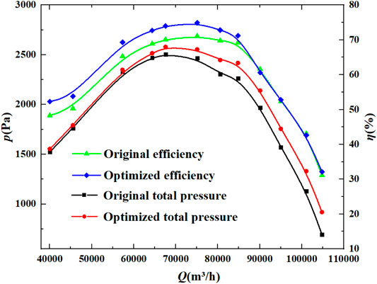
FIGURE 13. Fan performance curves original and optimized obtained by numerical simulation.

It can be seen from Figure 14A that the entropy of the fan between the leaves of the IGVs is relatively large before the optimization, and the distributions are similar in 0.1 span, 0.5 span and 0.9 span. The leading edge of the moving blades has obvious entropy change, mainly caused by the displacement and impact of the air-flow when the fan is working. At the same time, an area of greater entropy is formed on the suction surface of the rotor blade. The area with larger entropy value is also the area with more reflux, which is prone to vortex noise. After optimization, the entropy of the fan is significantly reduced. The entropy value of each area is reduced, especially in the IGVs duct, the entropy value between the leaves is significantly reduced. At the same time, at 0.9Span, the high entropy increase area of the suction surface of the bucket disappears, and the entropy value decreases. Small entropy can reduce eddy current noise, thereby improving the efficiency and stability of the fan.

FIGURE 14

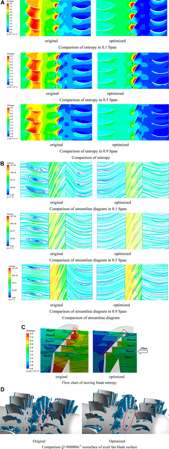
FIGURE 14. Comparative analysis of flow field results. Comparison of entropy in 0.1 Span comparison of entropy in 0.5 Span comparison of entropy in 0.9 Span (A) Comparison of entropy. Comparison of streamline diagram in 0.1 Span comparison of streamline diagram in 0.5 Span comparison of streamline diagram in 0.9 Span (B) Comparison of streamline diagram (C) Flow chart of moving blade entropy (D) Comparison Q=900000s⁻² isosurface of axail fan blade surface.

Obtain streamlines of 0.1, 0.5 and 0.9 Spans through the steady calculation results. Figure 14B show the comparison of the original and optimized streamlines. Streamlines can display the flow between fan stages based on velocity in the relative frame. There are obvious backflows and vortices between the IGVs and the OGVs of the 0.1Span original fan, causing flow loss and reducing fan efficiency. After the optimization model at 0.1 Span, the vortex between the IGVs disappears, and the number of vortices between the OGVs is significantly reduced. In 0.5Span and 0.9Span, the original fan has obvious backflow between the IGVs. The optimized fan eliminates the vortex and backflow between the IGVs, making the streamline more stable, and improving the aerodynamic performance and efficiency of the fan.

In order to compare the flow optimization before and after optimized, the streamlines and the contours of entropy on five selected planes (Plane 1 to Plane 5) are demonstrated in Figure 14C. These five planes are all produced nearly normal to the rotor tip chord direction. It can be seen from the figure that the entropy values on the suction side of the original fan is higher, and there is a larger vortex area at the tip of the blade. At the same time, the entropy value is larger at the leading edge and trailing edge of the moving blade, and the flow vortex is more obvious. After optimized, the five planes streamlines selected are smoother, and the entropy value is also significantly reduced, indicating that the internal flow characteristics of the fan have been greatly improved through optimization.

The Q isosurface can be used to judge the vortex distribution and vortex intensity around the fan. The way Q is defined (Hunt et al., 1988; Gang et al., 2020) is:

$Q=\frac{1}{2}\left({\omega }_{ij}^2-{\sigma }_{ij}^2\right)(19)$

${\omega }_{ij}=\frac{1}{2}\left(\frac{\partial u_i}{\partial x_j}-\frac{\partial u_j}{\partial x_i}\right)(20)$

${\sigma }_{ij}=\frac{1}{2}\left(\frac{\partial u_i}{\partial x_j}+\frac{\partial u_j}{\partial x_i}\right)(21)$

Where: ${\omega }_{ij}$ is the rotational angular velocity of the fluid; ${\sigma }_{ij}$ is the deformation rate of the fluid. By using the Q criterion, the structure and position of the vortex core can be visually identified. Figure 14D shows an example of Q = 900000s⁻² to illustrate the difference in vortex structure before and after optimization.

The divergence of the Coriolis acceleration received by the airflow was the primary cause of airflow-induced noise. This was a manifestation of the vortex sound caused by the expansion of the vortex in the velocity field, i.e., the stretching and destruction of the vortex generates aerodynamic noise, as described by the vortex-acoustic expression in Eq. 22 (Chunxu et al., 2010)

$\left[c_0^{-2}\left({\sigma }^2/{\sigma }^{2}t\right)-{\nabla }^2\right]\mathit{H}=\text{div}\left(\mathit{\omega }\times \mathit{v}\right)(22)$

Where H is the total enthalpy of the fluid, w is the flow vortex vector, and v is the velocity vector. The basic factors affecting the flow are the tension and breakdown of the vortex. Because the overall velocity of the flow field does not change significantly, the turbulent vortex w has an appreciable influence on the noise of the fan. The left side of Eq. 22 represents the propagation of sound waves in the fluid, and the right side represents the source of the vortex sound. Theoretically, the airflow radiation noise in the vortex is related to the size of the vortex, and the size, changes, and movement of the vortex in the flow field can reflect the noise distribution of the radiated sound field. Therefore, decreasing the vorticity can reduce the aerodynamic noise generated by the stretching and squeezing of the vortex, thereby also reducing the fan noise.

As shown in Figure 14D, there are large-scale vortices between IGVs and moving blades, and the vortex core in the red circle disappears after optimization. And the vortex will occupy the space of the flow path and cause the deterioration of the flow field. The vortex core in the red circle disappears after optimization, so it can be inferred that the noise performance of the optimized fan is better than that of the original one. In order to verify this conjecture, the acoustic characteristics of the impeller original and optimized were tested.

Depending on the intake angle of attack, separation occurs on the ventral surface of the guide vane in the intake direction Figure 14D, which results in a clear separation vortex that occupies a larger flow channel space in the blade channel. The separation vortex continues to develop along the path of the blade, which deteriorates the downstream flow field. Figure 14D shows the optimized vorticity diagram. The size and distribution range of the separation vortex in this area were significantly reduced, which improved the internal flow structure of the fan. Meanwhile, there was no clear vortex at the tail of the optimized moving blades because of the weakened separation vortex interference.

From the perspective of the flow structure, the vortex between the blade stages can be reduced by optimized the guide vanes, and the size of the streamline vortex is also reduced. Combined with the vortex sound theory described above, it can be seen that the optimization of the flow structure can effectively improve the eddy current noise. Based on the optimization effect of the flow field, the simulation calculation of the noise optimization of the fan will be further carried out below.According to GB/T 3767-1996 “Acoustics-Sound Pressure Method to Determine the Sound Power Level of Noise Sources-Engineering Method for Approximate Free Field Above the Reflecting Surface” (GB/T 3767-1996, 1996), a hemispherical field unit with 19 field points was established. Figure 15 shows the sound pressure distribution cloud diagram of the 19 domain points near the center frequency point under rated conditions. The position of the ring line A in Figure 15A is 45° from the outlet of the fan, which the distance equal to the diameter away from the center of the outlet. The sound pressure distribution cloud diagram indicates that the sound pressure value is the largest near the ring line A, which gradually decreases toward both ends. Figure 15B shows that the sound pressure value in the area near loop line A decreased significantly after optimization, indicating that the optimized fan structure exhibits a better noise reduction effect.

FIGURE 15

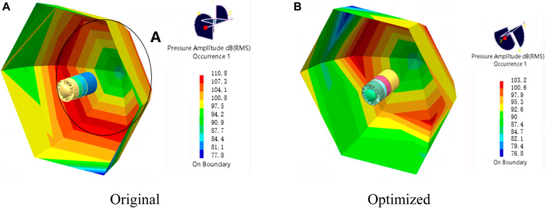
FIGURE 15. Comparison of the sound pressure distribution cloud diagram. (A) Original (B) Optimized.

Conclusion

This report describes the multi-objective optimization design of a large axial flow fan based on the MRGP model and verifies its feasibility and effectiveness through experiments and numerical simulations. The main conclusions from this work are as follows.

1) The MRGP model combined with a parameterization method was applied to optimize the design of the guide vanes in a large axial flow fan, which verified the feasibility of coupling the multi-Gaussian model and the multi-objective algorithm for the design of large axial flow fans. Comparison between the flow field and the sound field shows that the optimized fan flow field was more stable, and the strength of the eddy current on the flow direction is weakened, so the vortex-induced noise in the flow direction is also reduced. Through further experiments on the aerodynamic performance of the fan before and after optimization, it was found that the change trend of the performance curve of the fan after optimization is consistent with that of the original fan, and the total pressure and total pressure efficiency under different working conditions have been effectively improved. At the design working point, the total pressure increased by 144.4 Pa, the noise was reduced by 7.2 dB, and the low-frequency noise was also significantly reduced.

2) Under the premise of fewer design variables, this method revealed the coupling relationships between parameters and responses. The developed optimization process can be extended to optimize the designs of similar fluid machinery (Zhen et al., 2017).

Data Availability Statement

The original contributions presented in the study are included in the article/Supplementary Material, further inquiries can be directed to the corresponding author.

Author Contributions

Conceptualization, YH; methodology, YH; software, LL validation and SZ; writing—original draft preparation, YH; writing—review and editing, LL and ZG; project administration, SZ; funding acquisition, SZ.

Conflict of Interest

The authors declare that the research was conducted in the absence of any commercial or financial relationships that could be construed as a potential conflict of interest.

Publisher’s Note

All claims expressed in this article are solely those of the authors and do not necessarily represent those of their affiliated organizations, or those of the publisher, the editors and the reviewers. Any product that may be evaluated in this article, or claim that may be made by its manufacturer, is not guaranteed or endorsed by the publisher.

References

Baklacioglu, T., Turan, O., and Aydin, H. (2015). Dynamic Modeling of Exergy Efficiency of Turboprop Engine Components Using Hybrid Genetic Algorithm-Artificial Neural Networks. Energy 86, 709–721. doi:10.1016/j.energy.2015.04.025

CrossRef Full Text | Google Scholar

Burgos, M. A., Contreras, J., and Corral, R. (2009). “Validation of an Efficient Unstructured Time-Domain Rotor-Stator Interaction Method[C],” in Proceeding of the ASME Turbo Expo 2009: Power for Land, Sea, and Air, Orlando, Florida, USA, June 2009, 69–78.

Google Scholar

Carassale, L., Cattanei, A., Zecchin, F. M., and Moradi, M. (2020). Leakage Flow Flutter in a Low-Speed Axial-Flow Fan with Shrouded Blades. J. Sound Vibration 475, 115275. doi:10.1016/j.jsv.2020.115275

CrossRef Full Text | Google Scholar

Chen, W., and Zhou, Y. (2021). Research on Aerodynamic Noise of Tandem Double Cylinders Based on K-FWH Sound Comparison Method [J]. J. Beijing Univ. Aeronautics Astronautics 47 (10), 11. doi:10.13700/j.bh.1001-5965.2020.0365

CrossRef Full Text | Google Scholar

Chunxu, W., Tao, Z., and Guoxiang, H. (2010). Underwater Jet Noise Prediction Based on Vortex Sound Theory[J]. Ship Mech. 14 (6), 8. doi:10.3969/j.issn.1007-7294.2010.06.011

CrossRef Full Text | Google Scholar

Dittmar, J. H. (1972). Methods for Reducing Blade Passing Frequency Noise Generated by Rotor-Wake - Stator interaction[J].

Google Scholar

Gang, L., Lei, W., and Xiaomin, L. (2020). Numerical Study on the Influence of Tip Winglets on the Aerodynamic Performance and Noise Characteristics of Axial Flow Fans[J]. J. Xi'an Jiaotong Univ. 54 (7), 9. doi:10.7652/xjtuxb202007013

CrossRef Full Text | Google Scholar

GB/T2888-2008 (2008). Fan and Roots Blower Noise Measurement Method. Beijing: China Standard Press.

Google Scholar

Gb/T 1236-2017, (2017). Standardized Air Duct Performance Test for Industrial Ventilators. Beijing: China Standard Press.

Google Scholar

GB/T 3767-1996 (1996). Acoustics-Sound Pressure Method to Determine the Sound Power Level of Noise Sources-Engineering Method for the Approximate Free Field above the Reflecting Surface. Beijing: China Standard Press.

Google Scholar

Hassan, R. A., and Crossley, W. A. (2015). Multi-Objective Optimization of Communication Satellites with Two-Branch Tournament Genetic Algorithm[J]. J. Spacecraft Rockets 40 (2), 266–272. doi:10.2514/2.3942

CrossRef Full Text | Google Scholar

Hayat, T., Qayyum, S., Shehzad, S. A., and Alsaedi, A. (2018). Cattaneo-Christov Double-Diffusion Theory for Three-Dimensional Flow of Viscoelastic Nanofluid with the Effect of Heat Generation/absorption. Results Phys. 8, 489–495. doi:10.1016/j.rinp.2017.12.060

CrossRef Full Text | Google Scholar

Hunt, J., Wray, A. A., and Moin, P. (1988). “Eddies, Streams, and Convergence Zones in Turbulent Flows[J],” in Proc. CTR Summer Program, December 1988 (Stanford University).

Google Scholar

Hyuk, J. J., and Won-Gu, J. (2019). Analysis on Hub Vortex and the Improvement of Hub Shape for Noise Reduction in an Axial Flow Fan[C]. Department Mech. Eng. 259 (9), 472–481. doi:10.1007/s12206-020-0617-2

CrossRef Full Text | Google Scholar

Imtiaz, M., Kiran, A., Hayat, T., and Alsaedi, A. (2018). Three-dimensional Unsteady Flow of Maxwell Fluid with Homogeneous–Heterogeneous Reactions and Cattaneo–Christov Heat Flux[J]. J. Braz. Soc. Mech. Sci. Eng. 40 (9), 1–11. doi:10.1007/s40430-018-1360-9

CrossRef Full Text | Google Scholar

Jingyin, L., Weiwei, C., and Feng, L. (2010). Numerical Study of a New Type of Reversible Axial Flow Fan with Front and Rear Guide Vanes[J]. Chin. J. Mech. Eng. 46 (002), 139–144. doi:10.3901/JME.2010.02.139

CrossRef Full Text | Google Scholar

Jung, Y., Choi, M., Park, J-Y., and Baek, J. H. (2013). Effects of Recessed Blade Tips on the Performance and Flow Field in a Centrifugal Compressor[J]. Proc. Inst. Mech. Eng. A J. Power Energ. 227 (a2), 157–166. doi:10.1177/0957650912465278

CrossRef Full Text | Google Scholar

Kim, J. K., and Oh, S. H. (2018). A Study on the Structure of Instantaneous Flow Fields of a Small-Size Axial Fan by Large Eddy Simulation[J]. J. Korean Soc. Power Syst. Eng. 22, 28–35. doi:10.9726/kspse.2018.22.6.028

CrossRef Full Text | Google Scholar

Li, Y., Ouyang, H., and Du, Z. H. (2007). Optimization Design and Experimental Study of Low-Pressure Axial Fan with Forward-Skewed Blades[J]. Int. J. Rotating Machinery 2007 (1), 10. doi:10.1155/2007/85275

CrossRef Full Text | Google Scholar

Li, Y., Ye, Q., Liu, A., Meng, F., Zhang, W., Xiong, W., et al. (2017). Seeking Urbanization Security and Sustainability: Multi-Objective Optimization of Rainwater Harvesting Systems in China. J. Hydrol. 550, 42–53. doi:10.1016/j.jhydrol.2017.04.042

CrossRef Full Text | Google Scholar

Li, W., Yue, W., Huang, T., and Ji, N. (2021). Optimizing the Aerodynamic Noise of an Automobile Claw Pole Alternator Using a Numerical Method. Appl. Acoust. 171, 107629. doi:10.1016/j.apacoust.2020.107629

CrossRef Full Text | Google Scholar

Liu, H., Lee, S., Kim, M., Shi, H., Kim, J. T., Wasewar, K. L., et al. (2013). Multi-objective Optimization of Indoor Air Quality Control and Energy Consumption Minimization in a Subway Ventilation System. Energy and Buildings 66 (nov.), 553–561. doi:10.1016/j.enbuild.2013.07.066

CrossRef Full Text | Google Scholar

Liu, R., Li, J., Fan, J., Mu, C., and Jiao, L. (2017). A Coevolutionary Technique Based on Multi-Swarm Particle Swarm Optimization for Dynamic Multi-Objective Optimization[J]. Eur. J. Oper. Res. 261, 1028–1051. doi:10.1016/j.ejor.2017.03.048

CrossRef Full Text | Google Scholar

Moaveni, B. (1999). S. Finite Element Analysis Theory and Application with ANSYS [M]. Beijing, China: Prentice-Hall.

Google Scholar

Okiishi, T. H., Junkhan, G. H., and Serovy, G. K. (1970). “Experimental Performance in Annular Cascade of Variable Trailing-Edge Flap, Axial-Flow Compressor Inlet Guide Vanes[C],” in Proceeding of the Asme International Gas Turbine Conference & Products Show, Brussels, Belgium, May 1970, 8.

Google Scholar

Pogorelov, A., Meinke, M., and Schröder, W. (2016). Effects of Tip-gap Width on the Flow Field in an Axial Fan[J]. Int. J. Heat Fluid Flow 61, 466–481. doi:10.1016/j.ijheatfluidflow.2016.06.009

CrossRef Full Text | Google Scholar

Quin, D., Grimes, R., Walsh, E., Davies, M., and Kunz, S. (2004). “The Effect of Reynolds Number on Microfan Performance[C],” in Proceeding of the ASME 2004 2nd International Conference on Microchannels and Minichannels, New York, USA, June 2004, 81–86.

Google Scholar

Rufu, H., and Hongwu, Y. (1998). Research on Reducing Mutual Interference Noise between Moving Blades and Stationary Blades [J]. J. Huainan Mining Inst. 17 (4), 6. CNKI:SUN:HHJS.0.1998-02-020.

Google Scholar

Thongsri, J., and Pimsarn, M. (2015). Optimum Airflow to Reduce Particle Contamination inside Welding Automation Machine of Hard Disk Drive Production Line. Int. J. Precis. Eng. Manuf. 16 (3), 509–515. doi:10.1007/s12541-015-0069-2

CrossRef Full Text | Google Scholar

Varade, V., Agrawal, A., Prabhu, S. V., and Pradeep, A. M. (2015). Velocity Measurement in Low Reynolds and Low Mach Number Slip Flow through a Tube. Exp. Therm. Fluid Sci. 60, 284–289. doi:10.1016/j.expthermflusci.2014.10.001

CrossRef Full Text | Google Scholar

Wang, E., Zhang, H., Fan, B., Ouyang, M., Yang, K., Yang, F., et al. (2015). 3D Numerical Analysis of Exhaust Flow inside a Fin-And-Tube Evaporator Used in Engine Waste Heat Recovery. Energy 82, 800–812. doi:10.1016/j.energy.2015.01.091

CrossRef Full Text | Google Scholar

Zengming, Y., Yixing, L., and Yehui, W. (2001). Optimization of Exit Airflow Angle α2 of Axial Flow Rotor Blade with Front Guide Vane[J]. Fluid Machinery 2001 (06), 11–13. doi:10.3969/j.issn.1005-0329.2001.06.003

CrossRef Full Text | Google Scholar

Zhang, Y., Wang, Y., and Li, J. (2019). Volume Flow Rate Optimization of an Axial Fan by Artificial Neural Network and Genetic Algorithm[J]. Open J. Fluid Dyn. 09 (3), 207–223. doi:10.4236/ojfd.2019.93014

CrossRef Full Text | Google Scholar

Zhen, J., Arendt, P. D., Apley, D. W., and Wei, C. (2017). Multi-response Approach to Improving Identifiability in Model Calibration[M]. Springer International Publishing.

Google Scholar

Zhou, G., Xu, K., and Liu, F. (2018). Grid-converged Solution and Analysis of the Unsteady Viscous Flow in a Two-Dimensional Shock Tube[J]. Phys. Fluids 30, 016102. doi:10.1063/1.4998300

CrossRef Full Text | Google Scholar

Zhou, H., Zhou, S., Gao, Z., Dong, H., and Yang, K. (2020). Blades Optimal Design of Squirrel Cage Fan Based on Hicks-Henne Function [J]. Proc. Inst. Mech. Eng. C: J. Mech. Eng. Sci. 235, 3844–3858. doi:10.1177/0954406220969728

CrossRef Full Text | Google Scholar

Glossary

FW-H Ffowcs Williams and Hawkings

c₀² Represents the sound velocity of the undisturbed fluid

C_D Profile drag coefficient is a constant

D Impeller diameter(mm)

H The total enthalpy of the fluid

IGVS Inlet guide blades

L_ref The reference length (m)

MRGP multiple-response Gaussian process

m₁ Number of IGVS

m₂ Number of OGV

OGV Outlet guide blades

O_pt LHD Optimal Latin hypercube design

P Motor input power(W)

p_tf Total pressure(Pa)

Q The fan volume flow (m³/h)

SPL Sound pressure level Sound pressure level(dB)

SPL Sound pressure level Sound pressure level(dB)

t Time(s)

$T_{ij}$ The fluid viscous stress tensor

Δt 1/(6n)

u_i The velocity components

V_ref The reference speed (m/s)

$V^{\text{'}}$ Maximum difference from free stream velocity in the wake (m/s)

V₀ Free-stream velocity at upstream blade-row inlet(m/s)

w The flow vortex vector

χ_i The space fixed coordinate system

y+ A dimensionless parameter

Y_wall The first layer of the wall

Z Number of moving blade

k The turbulent kinetic energy

ε The turbulent dissipation

v The fluid kinematic viscosity (m²/s)

ρ The air density(kg/m³)

μ Dynamic viscosity of the fluid(m²/s)

ρ_a The air density under test conditions(kg/m³)

σ_a The chord length of the guide blade(mm)

σ_b the distance between moving blade and IGVS (mm)

θ_a The tip deflection angle of the guide vanes (°)

θ_b The root deflection angle of the guide vanes (°)