 Li-Xia Chen
 Chao Yuan
 Jun-Long Zhao1
 Yu Ma
Yu Ma- 1Sino-French Institute of Nuclear Engineering and Technology, Sun Yat-sen University, Zhuhai, China
- 2School of Aeronautics and Astronautics, Sun Yat-sen University, Shenzhen, China
- 3Key Laboratory of Efficient Utilization of Low and Medium Grade Energy, MOE, School of Mechanical Engineering, Tianjin University, Tianjin, China
The flow and heat transfer characteristics of the lead–bismuth eutectic (LBE) (Prandtl number Pr = 0.025) passing over a circular cylinder at Re = 500 are studied by direct numerical simulation and compared with the case of the air (Pr = 0.71). This article makes two major contributions: (1) heat transfer characteristics for the LBE flowing past a circular cylinder. For the case of air, the results show that a similarity exists among the wake structure of instantaneous temperature, fluctuating temperature, and velocity. However, these fields differ severely for the case of LBE. The local time-averaged Nusselt number (
1 Introduction
As single-phase coolants with good performance, liquid metals are widely used in advanced nuclear reactor systems (Todreas and Kazim, 2011), chip cooling (Khalaj and Halgamuge, 2017; Muhammad et al., 2020), spallation particle sources (Batta et al., 2015), and other applications with extremely high heat loads. The larger thermal conductivity of liquid metals, resulting in a lower molecular Prandtl number (Pr ∼10−2), guarantees higher heat exchange efficiency. Unlike ordinary fluids (Pr ∼1), the temperature field in a flow of fluids with a low Pr differs significantly from its velocity field (Zhang et al., 2019), leading to many open problems in the understanding of the underlying physical mechanism and characteristics of its heat transfer.
Molten lead–bismuth eutectic (LBE), a typical kind of liquid metals, is the coolant in lead–bismuth alloy-cooled fast reactors, that is, LFRs, one of Gen IV reactors (Abram and Ion, 2008). In a helical coil steam generator of an LFR system, LBE in the shell side transfers the heat taken from the nuclear reactor core to the cooling water in the tube side, which makes it of great importance to analyze the flow and heat transfer behavior when LBE sweeps the tube bundle of the steam generator. The Pr of LBE under the operating conditions of LFRs is within the range of 0.01–0.03 (Greenspan et al., 2008; Concetta, 2015; Guo et al., 2015). Experimental researches on thermohydraulic characteristics of LBE have been widely carried out, and many heat transfer correlations have been derived (Knebel et al., 2002; Ma et al., 2006; Shen et al., 2021). However, data obtained by experimental techniques are yet insufficient. Limited by the opaque and strong corrosiveness of LBE and the current experimental measurement techniques, these experiments mainly focus on the pressure drop, temperature difference, and heat transfer coefficient, while the details of the temperature and velocity fields are difficult to measure (Marocco et al., 2012; Zhang et al., 2020). In addition, most experimental studies on the characteristics of flow and heat exchange focus on the pipes, annular cavities, or longitudinally flow through fuel rods (Lefhalm et al., 2004; Tarantino et al., 2008; Cho et al., 2011). Few researches on external flows such as LBE sweeping the tube bundle in a helical coil steam generator have been reported yet.
Computational fluid dynamics (CFD) (Versteeg and Malalasekera, 2007) can be divided into three categories, including the direct numerical simulation (DNS) method, the large eddy simulation method, and the Reynolds-averaged Navier–Stokes (RANS) method, which provides another research approach. As the most practical option of industrial relevance, the RANS method needs the least computational costs. The key issue in the RANS simulation of liquid metals such as LBE is the closure of the turbulent heat flux term. Simple gradient diffusion hypothesis (Weigand et al., 1997), generalized gradient diffusion hypothesis (Ince and Launder, 1989), second-moment closures (Roelofs, 2019), and Algebraic Heat Flux Model (AHFM) series models (Shams et al., 2019) have been put forward to solve this issue. Nevertheless, models based on gradient diffusion hypothesis provide reliable results only for fluids with a Pr in the order of unity. Second-moment closures and AHFM series models give reasonable results for fluids with a low Pr under simple configuration conditions. The performance of these models needs to be improved under complex configuration conditions such as flows with separations (De Santis and Shams, 2018).
In recent years, DNS has been used to study the fluids with a very low Pr due to the high-fidelity data it can provide (Roelofs et al., 2015). For example, Kawamura et al. (1998) and Kawamura et al. (1999) investigated the influence of Pr and Reynolds number (Re) on the turbulent heat transfer in a channel by means of DNS, the Pr of which varies from 0.025 to 5.0. Redjem-Saad et al. (2007) used DNS to analyze the flow and turbulent heat transfer characteristics of fluids with the Pr within the range of 0.026 to 1.0 in a pipe. DNS is also used in the simulation of forced and mixed convention in a backward-facing step under a uniform heat flux boundary condition for fluids with different Pr to study the influence of Pr on turbulent Pr (Prt) (Zhao et al., 2018). These studies have confirmed that the heat transfer characteristics of fluids with a low Pr are significantly different from those of fluids with Pr ∼1. Particular patterns of Prt and time constant ratio occur for fluids with a low Pr, especially when flow separation happens, thus bringing a necessity to look into it more deeply.
So far, researches on the flow and heat transfer characteristics of fluids with a low Pr by DNS focus on simple configurations such as a channel, backward-facing step, annular cavity, and pipes. Investigations on the characteristics of external flow and heat transfer such as the phenomenon when LBE sweeps the tube bundle have been rarely reported. High-fidelity data of temperature and velocity fields under these conditions are insufficient. In this article, the flow and heat transfer characteristics of LBE passing a circular cylinder, the basic unit of a tube bundle, are studied by DNS as the beginning of a series of research. In addition, the case of air is also simulated for comparison.
The rest of this article is organized as follows. In Section 2, the problem definition and the methodology are described. The detailed results and discussion about the Nusselt number (Nu), the temperature field, the further analysis of velocity and temperature defect laws in the wake, and so on, are presented in Section 3. The conclusions are given in Section 4.
2 Problem Description and Methodology
2.1 Problem Description
This article is focused on the heat transfer when high-temperature fluid passes a circular cylinder at a constant low temperature. Three-dimensional incompressible flows without buoyancy are investigated at Pr = 0.025 (LBE) and Pr = 0.71 (air), simulating the situation within a limited temperature variation range. The governing equations are nondimensionalized by such characteristics: the diameter of the cylinder (D), the velocity of inflow (U∞), the temperature difference between inflow and cylinder (T∞ − Twall), the characteristic time (D/U∞), the density of inflow (ρ∞), and the characteristic pressure (ρ∞U∞2). Dimensionless governing equations are written as follows:
where u is the velocity; t is the time; p is the pressure; and T is the temperature difference between local fluid temperature and the cylinder. All data and physical quantities in this article are nondimensionalized, if not particularly illustrated.
The computational domain is a cuboid (50D × 40D × 6D), and the origin of which is placed at the center of the cylinder, as shown in Figure 1. The outlet is set as a constant boundary condition with zero reference pressure. Periodic boundary condition is imposed in the spanwise direction of the domain.
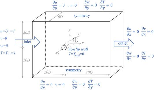
FIGURE 1. Schematic diagram of the computational domain and corresponding boundary conditions. u, v, and w represent the x-, y-, and z- components of u.
It should be noted that the thermal expansion rate of LBE is large, and the buoyancy should not be ignored under many operating conditions in LFRs. The physical properties of LBE are dependent on the temperature. Besides, Re in LFRs varies from zero to hundreds of thousands. However, every consideration mentioned previously causes extra burden on computational cost of DNS. Therefore, constant physical properties and moderate Re (Re = U∞D/ν = 500, where ν is the kinematic viscosity) without buoyancy are taken into consideration in this article as the beginning of a series of studies. Even in such cases, the present study still provides significantly important information for the liquid metals with very low Pr, especially when the temperature variation is within a limited range.
2.2 Numerical Schemes
The governing equations are discretized by the finite volume method and solved via the open-source CFD software OpenFOAM. The convergence criterion for all equations is 10−7. The time derivative term is discretized by Euler method. The convection and diffusion terms are discretized by Gauss QUICK scheme and Gauss linear corrected scheme, respectively. The pressure–velocity decoupling is dealt by PISO (pressure implicit with splitting of operators) algorithm. The preconditioned conjugate gradient method with geometric–algebraic multigrid (GAMG) as the preconditioner and diagonal incomplete Cholesky as the smoother are used to solve the pressure equation. The merge level in GAMG is chosen to be 2 to speed up the solving process.
2.3 Numerical Settings and Grid Independence Validation
Two sets of mesh with different resolutions are generated, and three cases are carried out: Pr = 0.71 with mesh A, Pr = 0.71 with mesh B, and Pr = 0.025 with mesh B, where the two cases of the air (Pr = 0.71) are used for mesh independence validation. The detailed settings of mesh A and B are listed in Table 1, and a view of mesh B is presented in Supplementary Figure S1. Uniform nodes are configured in the spanwise direction. Both sets of mesh are refined near the wall and in the wake region. The time step for the cases with mesh A and mesh B are set to 6.25 × 10⁻⁴ and 5 × 10⁻⁴, respectively, where the Courant–Friedrichs–Lewy (CFL) number is within 0.14 for both cases, meeting the CFL limit (Jiang, 2020). Each case was simulated for 10 flow-through times (500 dimensionless time); that is, 104 vortex shedding cycles after the statistically steady state of turbulence were reached. The results presented below are analyzed using the latest 500 dimensionless time. In total, 400,000 CPU hours were consumed for the three cases via Tianhe-2 platform, the national supercomputer center in Guangzhou, China.
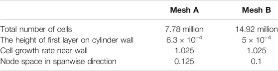
TABLE 1. Parameters of grid generation.
Table 2, Figure 2, and Supplementary Figure S2 provide some results for the case of Pr = 0.71. The meanings of involved symbols are as follows: dimensionless wall distance

TABLE 2. y+, St,

FIGURE 2. Statistical convergence of
Evidences are found from Table 2 that both sets of grids meet the number and refinement requirements in the boundary layer as the circumferentially averaged y+ in both cases is smaller than 0.1. The simulated results of St,
Therefore, mesh B was selected as the mesh for the case of Pr = 0.71. In a forced convection, the mesh resolution is determined by the velocity field when Pr < 1; therefore, there is no need to carry out the grid independence validation for the case with LBE. Accordingly, the data and analysis in the following sections are based on mesh B for both Pr = 0.025 and Pr = 0.71 cases. The above validation shows evidences that the numerical mesh resolution used in this study is adequate to simulate the fluid flow and heat transfer in the near wall region and the main stream region.
3 Results and Discussion
3.1 Forces on the Cylinder
In this article, the velocity and pressure relevant results are discussed regardless of Pr, as the temperature is considered as a passive scalar; that is, the heat transfer under different Pr has no effect on the flow field.
Temporal evolutions of the lift coefficient CL and drag coefficient CD are shown in Supplementary Figure S3 and Supplementary Figure S4, where
In Supplementary Figure S6, the variations of the time-averaged skin-friction coefficient
3.2 Instantaneous Fields and Vortex Structure
Instantaneous fields and the vortex structure of the two cases are demonstrated in Figure 3 and Figure 4, wherein the vortex structure is visualized via Q method (Jinhee and Hussain, 1995). The isosurface of Q = 0.2 indicates that the flow develops three-dimensionally in the near-wake region, where the vortices form a wavy spanwise structure, as revealed in Figure 3. For the case of air, a similarity among the wake structure of instantaneous temperature, fluctuating temperature, and velocity exists as Pr is close to 1 (Figure 4). The larger Pr gives a result that the influence of wall temperature spreads to a thinner region. Therefore, the temperature rapidly recovers to close to T∞ within about 2D downstream of the cylinder. On the contrary, the Pr of LBE is much smaller than 1, which leads to a significant enhancement of the diffusion effect. The instantaneous temperature field and the fluctuating temperature field differ severely from the velocity field (Figure 4).
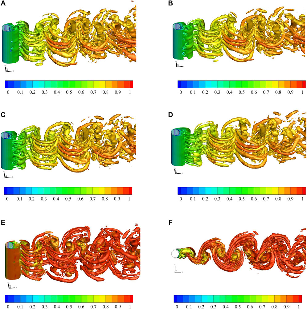
FIGURE 3. Instantaneous vortex shown by isosurfaces of Q = 0.2 for five instants of time. Note that these five instants stand for five typical moments in one vortex shedding period since the vortex shedding period tvs is 4.854 (according to the value of St in Table 2). In A–D, the isosurfaces are colored by the temperature for the case of LBE (Pr = 0.025). In E and F, the isosurfaces are colored by the temperature for the case of air (Pr = 0.71). (A) t = t0 (a typical moment), (B) t = t0 + 1, (C) t = t0 + 2, (D) t = t0 + 3, (E) t = t0 + 4, and (F) t = t0 + 4.
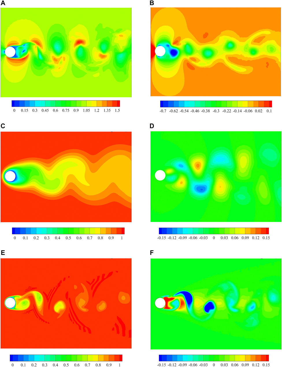
FIGURE 4. Distributions of pressure, velocity and temperature at a typical moment (at z = 0 plane). (A) Magnitude of velocity; (B) pressure; (C) transient temperature (LBE, Pr = 0.025); (D) fluctuating temperature T′ (T′ = T −
3.3 Nusselt Number
Figure 5A and Table 3 show the information of the local
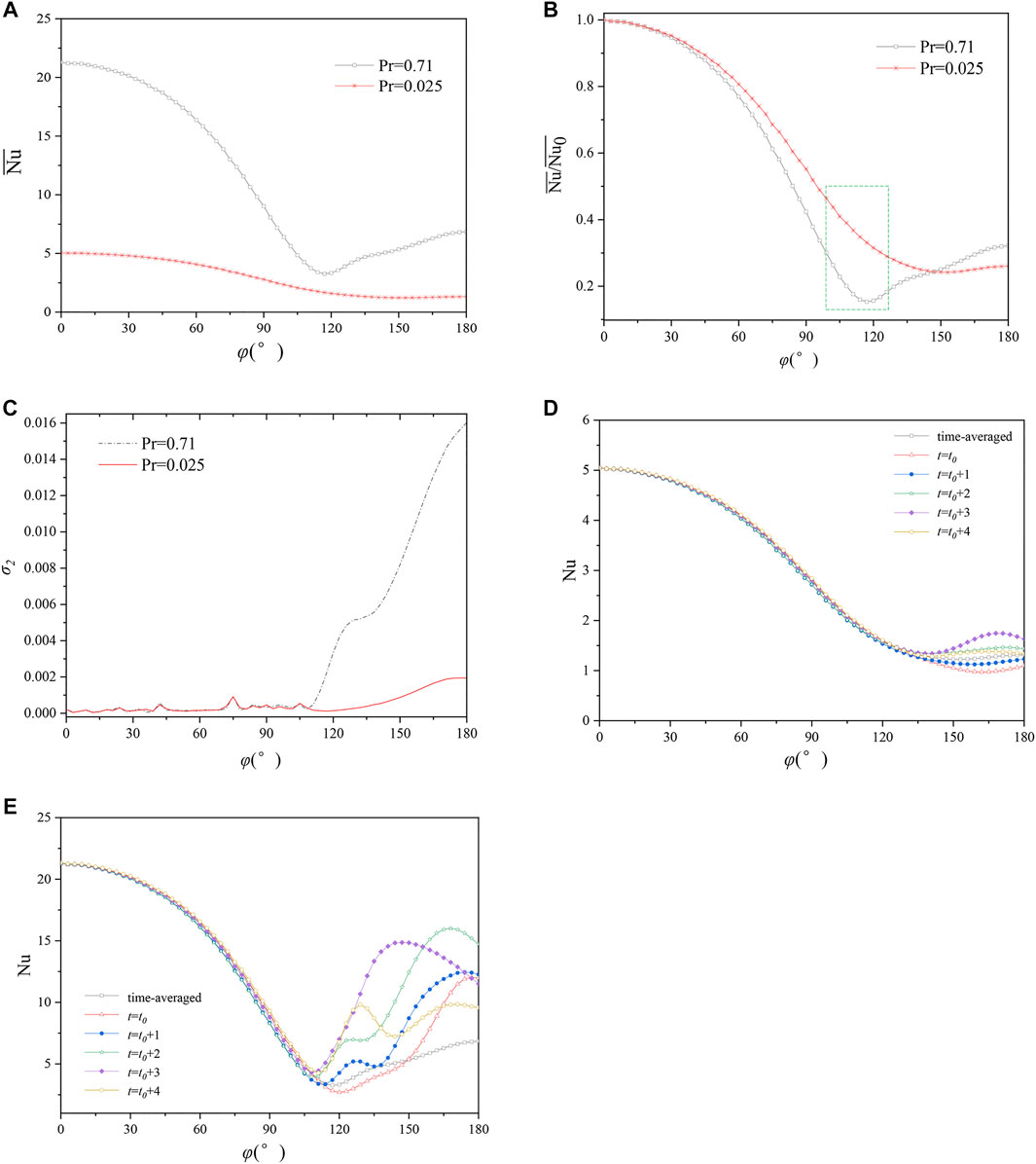
FIGURE 5. Distribution of Nu. The five instants of time in D and E are explained in Figure 3. (A) Variation of local
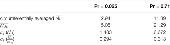
TABLE 3.
The parameter σ1 in Table3 is the circumferentially standard deviation, which reflects the circumferential uniformity. Results show that σ1 (
On the other hand, the two curves in Figure 5B almost coincide with each other when φ < 50° and then separate beyond this range, which can be explained together with Supplementary Figure S6 and Eq. 3. In the regions of φ < 50°,
Considering
where the subscript “n” represents the normal component, it is obvious that
The parameter σ2 in Figure 5C represents the standard deviations in the spanwise direction. For both cases, the values of σ2 are almost equal and smaller than 0.001 when φ < 110°, demonstrating a uniform spanwise distribution of
The comparison between local
3.4 Characteristics of Temperature Field
The characteristics of the time-averaged temperature field are shown in Figure 6. The mean temperature boundary layer is thicker for the case of LBE; therefore, the time-averaged temperature
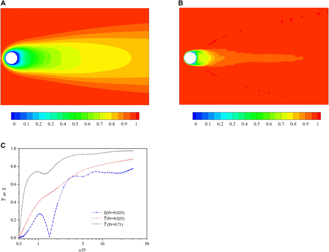
FIGURE 6. Distributions of time-averaged temperature fields. (A)
The R.M.S. of T′ and the turbulence kinetic energy k (
FIGURE 7. Distributions of root mean square fields. (A) T′rms on the plane of z = 0 (LBE, Pr = 0.025); (B) T′rms on the plane of z = 0 (air, Pr = 0.71); (C) k on the plane of z = 0; (D) variation of T′rms along the wake axis.
The transverse distribution of mean temperature and T′rms at different downstream locations are displayed in Figure 8. For the case of LBE, the distribution of
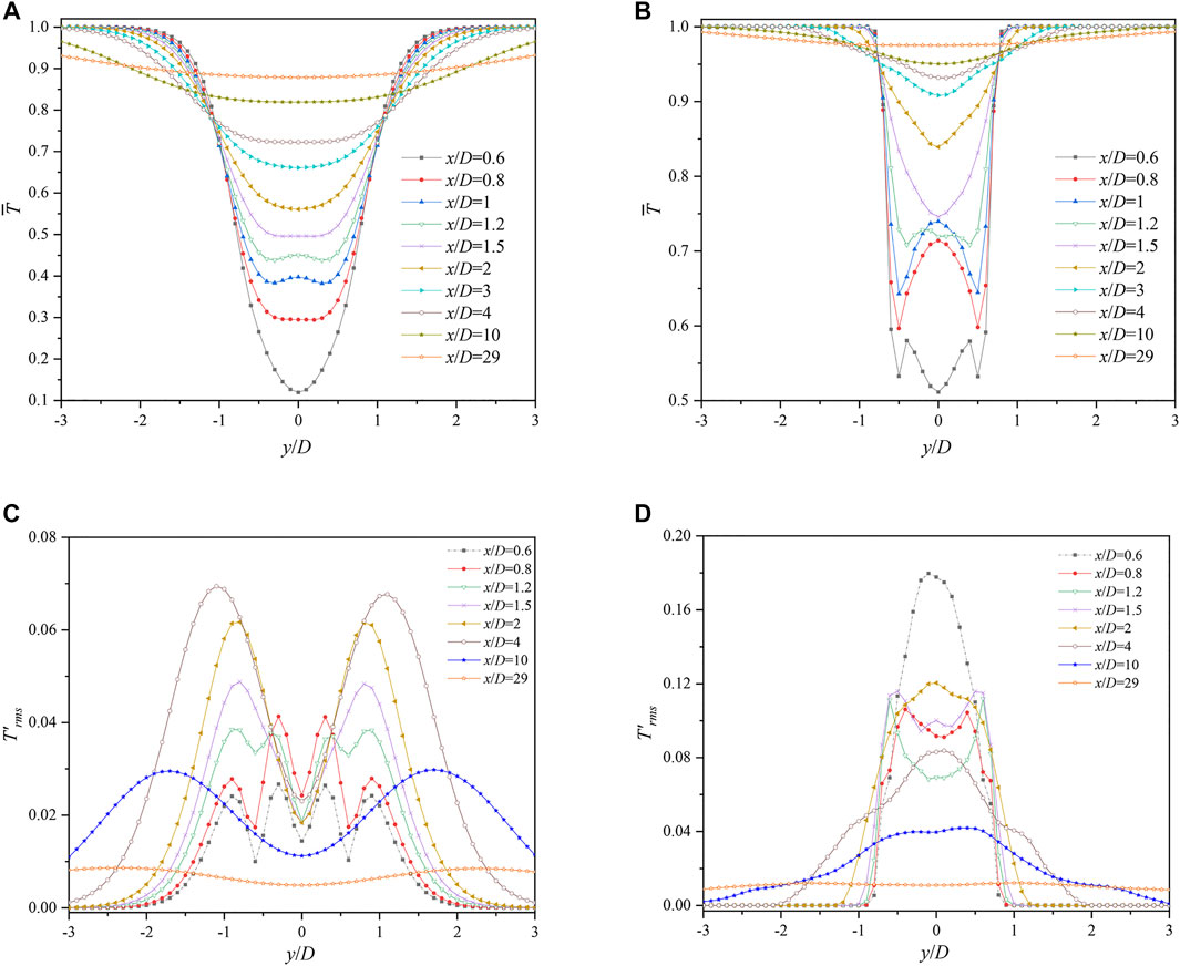
FIGURE 8. Transverse distributions of
For LBE, T′rms near the cylinder (x/D = 0.6–1) is smaller than those at x/D = 1.5–4. Four peaks appear at x/D ≤ 1.2, and double peaks for other locations. However, only one peak occurs for air at almost all x-locations, except for x/D = 0.8–1.5. T′rms near the wall (x/D = 0.6) is the largest. The attenuation rate of T′rms in the transverse direction in the LBE is smaller than that in the air.
These circumstances match with Figure 7 and Figure 4. The fluctuation of the temperature in the air is mostly dependent on the fluctuation of velocity; hence, a resemblance between the distribution of T′rms and k can be recognized. The wake structure of instantaneous and fluctuating temperature is close to Karman vortex, and the vortices on both sides affect the wake axis. Therefore, the transverse maxima of T′rms appears on the wake axis for most of streamwise locations. However, none of such wake structures can be observed from the fields of instantaneous temperature and fluctuating temperature for the case of LBE. The temperature fluctuation mainly occurs on both sides of the wake axis, resulting in four or double peaks in the transverse direction as shown in Figure 8C.
The fluctuations of typical variables near the cylinder wall are also discussed. In general, there is one local maximum for the cases with small angles, whereas two for other curves with larger angles, as illustrated in Figure 9, where Δr is the radial distance to the wall. The first local maximum or the first plateau is attributed to the wall effect, and the second one is due to vortex shedding. However, the characteristics of temperature fluctuations in the air and LBE are different.
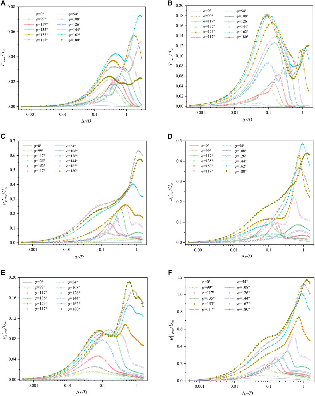
FIGURE 9. Distributions of several variables along different angles near the cylinder wall. (A) T′rms/T∞ for the case of LBE; (B) T′rms/T∞ for the case of air; (C) uφ′rms/U∞, where uφ means the circumferential component of velocity; (D) ur′rms/U∞, where ur means the radial component of velocity; (E) w′rms/U∞; (F) |u|′rms/U∞.
The transition angle from one maximum to two maxima for T′rms/T∞ in the air is approximately 117°, a little larger than the flow separation angle, which is comparable with Figure 5E. T′rms/T∞ almost increases with the increase in φ, and the first maximum occurs where Δr/D = 0.05–0.15. The radial component of the gradient of temperature is quite large, as can be seen from the contours of temperature (Figure 4), so that the radial variations of temperature are relevant to the fluctuations of ur. Therefore, between Figure 9B and Figure 9D, some similarities of the transition angle and the locations where the first maximum or the first plateau occurs can be observed. It should be noted that first peaks in the near wall region in the graph of uφ′rms/U∞ (Figure 9C), ur′rms/U∞ (Figure 9D), and |u|′rms/U∞ (Figure 9F) are not obvious, resulting from the fact that the diffusion and convection are significantly enhanced in the flow separation region.
T′rms/T∞ of LBE is smaller than that of air. The transition angle from one maximum to two maxima for T′rms/T∞ in the LBE is approximately 135°, which is much larger than the flow separation angle, and the phenomenon is comparable with Figure 5D. Unlike the case of air, the second peak of T′rms/T∞ is larger than the first peak/plateau for the case of LBE, because the smaller Pr of LBE causes a more significant suppression of temperature fluctuation by the wall. The locations where the first maximum or the first plateau of T′rms/T∞ occurs are Δr/D = 0.2–0.6, further than T′rms/T∞ in air and uφ′rms/U∞ for both cases.
3.5 Temperature and Velocity Defect Laws in Wake
The velocity and temperature profiles in the near-wake region are determined by the boundary layer, the shape of the object, and whether a flow separation occurs. There exists a similarity of the velocity or temperature profile in the far wake of a bluff body such as x/D > 50 (Zdravkovich, 1997) or x/D > 100 (Chen, 2002), where the disturbance of the object on the flow or temperature field tends to vanish. It should be noted that this location where the self-preserving flow exists depends on how far it needs to develop the profile from a boundary layer type at the trailing edge of the object to a fully developed similar wake profile. Therefore, this distance is closely related to the specific working conditions. In other words, it has been well established that there exists a velocity scale and a length scale, which are the universal function of x/D, scaled by which the mean velocity profiles and the mean temperature profiles may be self-similar (Wygnanski et al., 1986). The existence of such similar temperature scale under a specific condition or not is a matter to be discussed.
The transverse profile of velocity defect follows the Gaussian distribution for a small-defect wake in a two-dimensional plate wake, detailed deductions of which can be found in the references (Wygnanski et al., 1986; Chen, 2002). In this section, the self-preserving states of the temperature and velocity in the wake are discussed according to the simulation cases by introducing the velocity defect as the velocity scale, the temperature defect as the temperature scale, and the defect width as the length scale, respectively. The similarity or deviation between the Gaussian distribution and the transverse profiles of velocity defect and temperature defect are also discussed.
3.5.1 Velocity Defect, Temperature Defect and Defect Width
The velocity defect along the transverse direction at the downstream position of x/D is defined as follows:
where the defect variable udf is marked by the subscript “df”, and
where udf+ is the normalized velocity defect, udf,c is the velocity defect on the wake axis, that is, the transverse center of the wake, at the downstream location of x/D, and
Correspondingly, the temperature defect Tdf and normalized temperature defect Tdf+ are calculated as follows:
where
Assume that the transverse profile of velocity defect follows the Gaussian distribution, as expressed in Eq. 11. Then the Gaussian parameter σU can be obtained by fitting Eq. 11 with the simulation results of y and udf+. The velocity defect width of wake WU is defined as half of the wake width where udf+ = 1%; that is, WU satisfies that
Figure 10A presents how WU and WT vary with the distance from the cylinder. The variation trends of WT (Pr=0.71) and WU are similar. They increase near the cylinder, experience a plateau in the range of x/D = 3–6, and then keep increasing along the downstream. However, no plateau can be observed for WT (Pr=0.025). In the entire wake, WT (Pr=0.025) > WT (Pr=0.71) > WU, which is consistent with the results shown in the contour of time-averaged temperature field (Figures 6A, B). In LBE, the region where the cylinder influences the temperature in the transverse direction is large. On the contrary, the effect is confined in a very narrow range for the case of air. The transverse influence range of temperature in the LBE is 1.4–2.2 times of that for the air case.
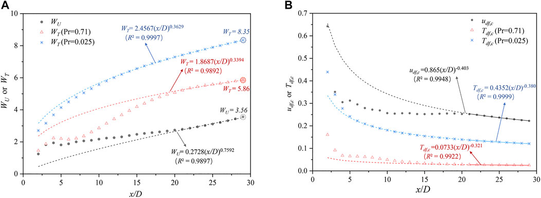
FIGURE 10. Variations of velocity defect width, temperature defect width, velocity defect, and temperature defect in wake. The curves and formulas are fitting results according to the data at locations of x/D ≥ 21 and R2 represents the coefficient of determination. (A) Defect width; (B) velocity defect and temperature defect.
The defect width should be proportional to (x/D)0.5 according to the mathematical model of the far wake with the introduction of linear hypothesis during deduction (Zdravkovich, 1997) and the unknown influence of Pr bring about a necessity of studies on whether the relationship is still established for the wake of cylinder and the scope of the establishment. The power–law relationships fitted by the data of far wake (x/D ≥ 21) are shown in Figure 10A. For the case of LBE, it is obvious that WT = 2.4567 (x/D)0.3629 is almost valid in the whole wake, except for slight deviations at x/D < 5. However, the results for WT (Pr=0.71) and WU deviate sharply from the fitting curves when x/D < 21. It can be concluded that the self-preserving state of temperature appears from the near-wake region (x/D ≥ 5) for the case of LBE, while only in far wake (x/D ≥ 21) for the self-preserving states of temperature in the air and velocity.
Another notable thing is that even though the data of defect width in far wake satisfy the power–law relationships well, which has been validated in Figure 10A by the fact that R2 is close to 1 for the three cases, especially for WT (Pr=0.025), the power–law coefficients differ from the theoretical value 0.5. The main reason is that some assumptions derived from the theory are different from the calculation conditions in this article. For example, the flow and temperature fields in this article are three-dimensional, not two-dimensional, and the observed region is not small-defect wake. This also reflects that the results of the theoretical derivation based on assumptions are not always applicable to the complicated situations such as the flow and heat transfer around a circular cylinder.
The following is to discuss the velocity scale and temperature scale. Figure 10B shows the relationships between udf,c or Tdf,c and x/D on the wake axis. The exponents of formulas for udf,c, Tdf,c (Pr = 0.71), and Tdf,c (Pr = 0.025) are −0.403, −0.321, and −0.380, respectively, which are close to −0.5 with some deviations. As shown in Figure 10A, the power law describes the distribution of Tdf,c well within the range of x/D = 5–30 in the LBE, but x/D > 15 for the case of air.
3.5.2 Transverse Profiles and Fluctuation Attenuation
As explained previously, the transverse profiles of velocity defect follow the Gaussian distribution for a small-defect wake (Wygnanski et al., 1986), that is, the region where udf,c
The normalized transverse coordinates YT and YU, defined as follows, are introduced to illustrate the difference of profiles more clearly,
where yi is the y-coordinate at the location of xi; WT,i and WU,i are the temperature defect width and velocity defect width at the location of xi, respectively. The profiles of normalized temperature defect Tdf+ and normalized velocity defect udf+ with YU and YT are plotted in Figures 11A–C, respectively. Considering the symmetry of the time-averaged field, the results of YU < 0 or YT < 0 are not shown here. According to Eq. 11–Eq. 16, these profiles collapse quite neatly onto a single curve described by the following formula:
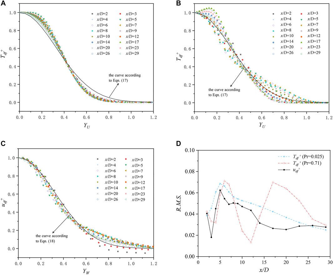
FIGURE 11. Transverse profiles of normalized temperature defect and normalized velocity defect. (A) Tdf+ in the LBE, Pr = 0.025; (B) Tdf+ in the air, Pr = 0.71; (C) udf+; (D) R.M.S. of differences.
Figure 11 illustrates that the Gaussian distribution describes the profiles roughly with certain deviations presented by the R.M.S. of differences shown in Figure 11D.
The pattern of how the relative fluctuations on the wake axis decay, which stands for the dynamic similarity, is investigated before the discussions about the reasons of the deviations in Figure 11. The attenuation profiles of T′rms/Tdf,c, u′rms/udf,c, v′rms/udf,c, and w′rms/udf,c on the wake axis are given in Figure 12, where three stages can be generally observed. First, all relative fluctuations increase rapidly in the near-wake vortex street formation zone until x/D ≈ 5, and then different trends appear after that. Apart from a slight decrease near the location of x/D ≈ 5, T′rms/Tdf,c in the LBE almost maintains until the end of the computational domain, which means that the temperature of LBE experiences self-preserving state in this region. T′rms/Tdf,c in the air keeps declining rapidly after the peak at x/D ≈ 5, and the attenuation rate decreases from x/D ≈ 25, implying that the self-preserving state for the temperature in the air does not appear until x/D ≈ 25. Three components of velocity differ significantly in the entire wake and converge gradually at the end of the computational domain, indicating that the self-preserving state for the velocity does not show up within x/D < 30.
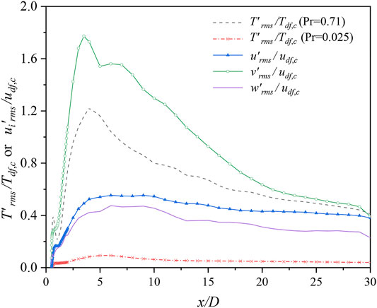
FIGURE 12. Distribution of T′rms/Tdf,c, u′rms/udf,c, v′rms/udf,c and w′rms/udf,c on wake axis.
The fact that the linear hypothesis introduces an assumption that udf,c
The distribution of Tdf+ for the air in Figure 11B is not centralized; therefore, the R.M.S. in Figure 11D is quite large until x/D > 25. The Gaussian distribution tends to overestimate Tdf+ when YT < 0.4 and underestimate it when YT > 0.4 in the region of x/D < 10. Opposite phenomenon is observed in the region of x/D > 12. A local descent appears in the region of 6 < x/D < 12 in Figure 11D due to the presence of transition region 10 < x/D < 12. The descent of the attenuation rate of T′rms/Tdf,c (shown in Figure 12) corresponds to the smaller R.M.S. of difference for air in Figure 11D when x/D > 25.
The R.M.S. of Tdf+ for the case of LBE in Figure 11D declines continuously when x/D > 5; therefore, the transversal profiles are well centered as it is under a self-preserving state. Even so, differences from the Gaussian distribution can be observed in Figure 11A, in which it tends to overestimate Tdf+ when YT > 0.4 and underestimate it near the center of the wake. However, the differences are reasonable, considering that Pr of LBE is much smaller than unity.
3.5.3 Summary
As can be seen from Figure 12 and Figure 11D, the attenuation of relative fluctuation is consistent with the trend of the deviation between normalized temperature/velocity defect and the Gaussian distribution for the temperature in the LBE, the temperature in the air, and the velocity, except for the local descent in Figure 11D as explained above. In addition, Figure 10 shows that the sum of the exponents of temperature defect and temperature defect width is close to zero for both LBE and air cases, which is in good agreement with the law of “velocity defect width*velocity defect = constant” obtained from the wake of two-dimensional plate (Wygnanski et al., 1986; Zdravkovich, 1997), whereas the sum for the velocity deviates from zero. These results demonstrate that the velocity field has not entered the self-preserving state yet, whereas the self-preserving state starts from x/D = 5 for the temperature in the LBE and x/D = 21 for the temperature in the air, from another point of view.
It is obtained that the recovering length and the defect width of the temperature field of LBE flow show much larger than that of the conventional fluid flow (Pr close to 1). It indicates that in a helical coil steam generator, the flow and thermal boundaries may vary for pipes at different locations, and its performance will be significantly affected by the diameter, distance, and arrangement of the bundles. Improper design of bundle geometry may lead to uneven heat transfer, affect the heat exchange efficiency, and result in temperature hotspots. Therefore, a more adequate experimental/numerical verification is needed during the design of helical coil steam generators with LBE as the working fluid.
4 Conclusion
In this article, the flow and heat transfer characteristics of LBE (Pr = 0.025) and air (Pr = 0.71) passing a circular cylinder at Re = 500 are investigated by DNS method. The agreement of the numerical results with the literature verifies the effectiveness of the methodology. For the case of air, there exists a similarity among the instantaneous temperature, fluctuating temperature, and velocity fields in the wake downstream the cylinder, whereas these fields differ severely for the case of LBE. The temperature boundary layer of LBE is thicker than that of air. The downstream temperature is more affected by the wall temperature of the cylinder, and a large region of low temperature can be recognized. The main conclusions are as follows:
1) The circumferentially averaged
2) The temperature fluctuation of LBE is smaller in both the bulk region and the near wall region. A resemblance between the distribution of the R.M.S. of fluctuation temperature T′rms and the turbulence kinetic energy k can be recognized in the air, but it disappears for the case of LBE.
3) By introducing the velocity defect as the velocity scale, the temperature defect as the temperature scale and the defect width as the length scale, the self-preserving state and the similarity or deviation between the Gaussian distribution and the transverse profiles of velocity defect and temperature defect are fully discussed. It is found that the velocity field has not entered the self-preserving state yet, whereas the self-preserving state starts from x/D = 5 for the temperature in the LBE and x/D = 21 for the temperature in the air.
To obtain a more general database, the temperature calculated in this article is nondimensionalized. If extended to dimensional situations, these data will have a certain degree of confidence under the cases within a small temperature variation, where the influence of buoyancy can be ignored. For the case of large temperature difference, the influence of buoyancy cannot be ignored, and constant physical properties are inappropriate. In that way, further simulations are needed to determine the error quantitatively. Considering the amount of calculation, this will be carried out in future work.
In a reactor, LBE experiences various working conditions, including different flow rates and different temperatures. In the initial stage of the research, a series of databases with different Prs and an Re at low/medium level are carried out. Generation of a database with high Res and different Prs is ongoing. In the engineering field, database under an Re of 500 and different Prs can be used not only for comparison and verification with experimental results and RANS simulation, but also for the development of turbulence heat flux models, which will be extended to more complex conditions with higher Re with the supplementation of databases under other Re.
In conclusion, a fruitful description of the flow and heat transfer of the LBE passing a circular cylinder is presented, which is a typical flow in a helical coil steam generator of an LFR. Even without consideration of buoyancy, these highly resolved data on velocity and temperature are valuable for turbulence and heat fluxes modeling in the future, especially for liquid–metal flow with extremely low Prs within a limited variation range of operating temperature.
Data Availability Statement
The original contributions presented in the study are included in the article/Supplementary Material, further inquiries can be directed to the corresponding authors.
Author Contributions
Methodology, L-XC and H-NZ; Software, H-NZ, L-XC, and CY; Formal Analysis, L-XC, and J-LZ; Investigation, F-CL, L-XC, CY, and J-LZ; Supervision and resources, YM and F-CL; Writing—Original Draft, L-XC and CY; Writing—Review and Editing, L-XC, H-NZ, YM, and F-CL; Funding acquisition, J-LZ, H-NZ, YM and F-CL All authors have read and agreed to the published version of the manuscript.
Funding
This research was funded by the National Natural Science Foundation of China (Grant numbers 51976238, 51776057, 52006249 and U1830118) and the open fund project of Key Laboratory of Thermal Power Technology (Grant number TPL2018B02).
Conflict of Interest
The authors declare that the research was conducted in the absence of any commercial or financial relationships that could be construed as a potential conflict of interest.
Publisher’s Note
All claims expressed in this article are solely those of the authors and do not necessarily represent those of their affiliated organizations, or those of the publisher, the editors, and the reviewers. Any product that may be evaluated in this article, or claim that may be made by its manufacturer, is not guaranteed or endorsed by the publisher.
Supplementary Material
The Supplementary Material for this article can be found online at: https://www.frontiersin.org/articles/10.3389/fenrg.2022.823590/full#supplementary-material
References
Abram, T., and Ion, S. (2008). Generation-IV Nuclear Power: A Review of the State of the Science. Energy Policy 36, 4323–4330. doi:10.1016/j.enpol.2008.09.059
Batta, A., Class, A. G., Litfin, K., Wetzel, T., Moreau, V., Massidda, L., et al. (2015). Experimental and Numerical Investigation of Liquid-Metal Free-Surface Flows in Spallation Targets. Nucl. Eng. Des. 290, 107–118. doi:10.1016/j.nucengdes.2014.11.009
Cho, J. H., Batta, A., Casamassima, V., Cheng, X., Choi, Y. J., Hwang, I. S., et al. (2011). Benchmarking of thermal Hydraulic Loop Models for Lead-Alloy Cooled Advanced Nuclear Energy System (LACANES), Phase-I: Isothermal Steady State Forced Convection. J. Nucl. Mater. 415, 404–414. doi:10.1016/j.jnucmat.2011.04.043
Churchill, S. W., and Bernstein, M. (1977). A Correlating Equation for Forced Convection from Gases and Liquids to a Circular cylinder in Crossflow. J. Heat Transf. 99, 300–306. doi:10.1115/1.3450685
Concetta, F. (2015). Handbook on Lead-bismuth Eutectic Alloy and Lead Properties, Materials Compatibility, Thermal-hydraulics and Technologies. 2015 Edition. Paris: OECD.
De Santis, A., and Shams, A. (2018). Application of an Algebraic Turbulent Heat Flux Model to a Backward Facing Step Flow at Low Prandtl Number. Ann. Nucl. Energ. 117, 32–44. doi:10.1016/j.anucene.2018.03.016
Greenspan, E., Hong, S. G., Lee, K. B., Monti, L., Okawa, T., Susplugas, A., et al. (2008). Innovations in the ENHS Reactor Design and Fuel Cycle. Prog. Nucl. Energ. 50, 129–139. doi:10.1016/j.pnucene.2007.10.022
Guo, C., Lu, D., Zhang, X., and Sui, D. (2015). Development and Application of a Safety Analysis Code for Small Lead Cooled Fast Reactor SVBR 75/100. Ann. Nucl. Energ. 81, 62–72. doi:10.1016/j.anucene.2015.03.021
Habibi Khalaj, A., and Halgamuge, S. K. (2017). A Review on Efficient thermal Management of Air- and Liquid-Cooled Data Centers: From Chip to the Cooling System. Appl. Energ. 205, 1165–1188. doi:10.1016/j.apenergy.2017.08.037
Ince, N. Z., and Launder, B. E. (1989). On the Computation of Buoyancy-Driven Turbulent Flows in Rectangular Enclosures. Int. J. Heat Fluid Flow 10, 110–117. doi:10.1016/0142-727X(89)90003-9
Jeong, J., and Hussain, F. (1995). On the Identification of a Vortex. J. Fluid Mech. 285, 69–94. doi:10.1017/s0022112095000462
Jiang, H. Y. (2020). Separation Angle for Flow Past a Circular cylinder in the Subcritical Regime. Phys. Fluids 32, 014106. doi:10.1063/1.5139479
Kawamura, H., Abe, H., and Matsuo, Y. (1999). DNS of Turbulent Heat Transfer in Channel Flow with Respect to Reynolds and Prandtl Number Effects. Int. J. Heat Fluid Flow 20, 196–207. doi:10.1016/s0142-727x(99)00014-4
Kawamura, H., Ohsaka, K., Abe, H., and Yamamoto, K. (1998). DNS of Turbulent Heat Transfer in Channel Flow with Low to Medium-High Prandtl Number Fluid. Int. J. Heat Fluid Flow 19, 482–491. doi:10.1016/S0142-727X(98)10026-7
Knebel, J. U., Müller, G., and Konys, (2002). “Lead-Bismuth Activities at the Karlsruhe Lead Laboratory KALLA,” in International Conference on Nuclear Engineering (Arlington, VA: ASME). doi:10.1115/icone10-22240
Krall, K. M., and Eckert, E. R. G. (1973). Local Heat Transfer Around a Cylinder at Low Reynolds Number. J. Heat Transf. 95, 273–275. doi:10.1115/1.3450044
Lefhalm, C.-H., Tak, N.-I., Piecha, H., and Stieglitz, R. (2004). Turbulent Heavy Liquid Metal Heat Transfer along a Heated Rod in an Annular Cavity. J. Nucl. Mater. 335, 280–285. doi:10.1016/j.jnucmat.2004.07.028
Ma, W., Bubelis, E., Karbojian, A., Sehgal, B. R., and Coddington, P. (2006). Transient Experiments from the thermal-hydraulic ADS lead Bismuth Loop (TALL) and Comparative TRAC/AAA Analysis. Nucl. Eng. Des. 236, 1422–1444. doi:10.1016/j.nucengdes.2006.01.006
Marocco, L., Loges, A., Wetzel, T., and Stieglitz, R. (2012). Experimental Investigation of the Turbulent Heavy Liquid Metal Heat Transfer in the thermal Entry Region of a Vertical Annulus with Constant Heat Flux on the Inner Surface. Int. J. Heat Mass Transfer 55, 6435–6445. doi:10.1016/j.ijheatmasstransfer.2012.06.037
Muhammad, A., Selvakumar, D., and Wu, J. (2020). Numerical Investigation of Laminar Flow and Heat Transfer in a Liquid Metal Cooled Mini-Channel Heat Sink. Int. J. Heat Mass Transfer 150, 119265. doi:10.1016/j.ijheatmasstransfer.2019.119265
Norberg, C. (2003). Fluctuating Lift on a Circular cylinder: Review and New Measurements. J. Fluids Structures 17, 57–96. doi:10.1016/s0889-9746(02)00099-3
Redjem-Saad, L., Ould-Rouiss, M., and Lauriat, G. (2007). Direct Numerical Simulation of Turbulent Heat Transfer in Pipe Flows: Effect of Prandtl Number. Int. J. Heat Fluid Flow 28, 847–861. doi:10.1016/j.ijheatfluidflow.2007.02.003
Roelofs, F., Shams, A., Otic, I., Böttcher, M., Duponcheel, M., Bartosiewicz, Y., et al. (2015). Status and Perspective of Turbulence Heat Transfer Modelling for the Industrial Application of Liquid Metal Flows. Nucl. Eng. Des. 290, 99–106. doi:10.1016/j.nucengdes.2014.11.006
Roelofs, F. (2019). Thermal Hydraulics Aspects of Liquid Metal Cooled Nuclear ReactorsCambridge. Cambridge: Woodhead Publishing.
Shams, A., De Santis, A., and Roelofs, F. (2019). An Overview of the AHFM-NRG Formulations for the Accurate Prediction of Turbulent Flow and Heat Transfer in Low-Prandtl Number Flows. Nucl. Eng. Des. 355, 110342. doi:10.1016/j.nucengdes.2019.110342
Shen, Y., Peng, S., Yan, M., Zhang, Y., Deng, J., Yu, H., et al. (2021). Study of Flow and Heat Transfer Characteristics of Lead-Based Liquid Metals in a Turbulent Tube Flow and the Impacts of Roughness. Front. Energ. Res. 9, 634964. doi:10.3389/fenrg.2021.634964
Tarantino, M., De Grandis, S., Benamati, G., and Oriolo, F. (2008). Natural Circulation in a Liquid Metal One-Dimensional Loop. J. Nucl. Mater. 376, 409–414. doi:10.1016/j.jnucmat.2008.02.080
Todreas, N. E., and Kazim, M. S. (2011). Nuclear Systems Volume I: Thermal Hydraulic Fundamentals. 2nd edn. Boca Raton: CRC Press.
Versteeg, H. K., and Malalasekera, W. (2007). An Introduction to Computational Fluid Dynamics: The Finite Volume Method. Second Edition. Harlow: Pearson Education Limited.
Weigand, B., Ferguson, J. R., and Crawford, M. E. (1997). An Extended Kays and Crawford Turbulent Prandtl Number Model. Int. J. Heat Mass Transfer 40, 4191–4196. doi:10.1016/S0017-9310(97)00084-7
Wygnanski, I., Champagne, F., and Marasli, B. (1986). On the Large-Scale Structures in Two-Dimensional, Small-Deficit, Turbulent Wakes. J. Fluid Mech. 168, 31–71. doi:10.1017/S0022112086000289
Zdravkovich, M. M. (1997). Flow Around Circular Cylinders Volume 1 Fundamentals. New York: Oxford University Press.
Zhang, Y., Wang, C., Cai, R., Lan, Z., Shen, Y., Zhang, D., et al. (2020). Experimental Investigation on Flow and Heat Transfer Characteristics of lead-bismuth Eutectic in Circular Tubes. Appl. Therm. Eng. 180, 115820. doi:10.1016/j.applthermaleng.2020.115820
Zhang, Y., Wang, C., Lan, Z., Wei, S., Chen, R., Tian, W., et al. (2020). Review of Thermal-Hydraulic Issues and Studies of Lead-based Fast Reactors. Renew. Sustainable Energ. Rev. 120, 109625. doi:10.1016/j.rser.2019.109625
Keywords: lead–bismuth eutectic, flow over circular cylinder, direct numerical simulation, heat transfer, temperature defect law
Citation: Chen L-X, Yuan C, Zhao J-L, Zhang H-N, Ma Y and Li F-C (2022) Direct Numerical Simulation of Heat Transfer of Lead–Bismuth Eutectic Flow Over a Circular Cylinder at Re = 500. Front. Energy Res. 10:823590. doi: 10.3389/fenrg.2022.823590
Received: 27 November 2021; Accepted: 11 January 2022;
Published: 28 February 2022.
Edited by:
Wenxi Tian, Xi’an Jiaotong University, ChinaReviewed by:
Chenglong Wang, Xi’an Jiaotong University, ChinaWeihua Cai, Northeast Electric Power University, China
Copyright © 2022 Chen, Yuan, Zhao, Zhang, Ma and Li. This is an open-access article distributed under the terms of the Creative Commons Attribution License (CC BY). The use, distribution or reproduction in other forums is permitted, provided the original author(s) and the copyright owner(s) are credited and that the original publication in this journal is cited, in accordance with accepted academic practice. No use, distribution or reproduction is permitted which does not comply with these terms.
*Correspondence: Hong-Na Zhang, aG9uZ25hQHRqdS5lZHUuY24=; Yu Ma, bWF5dTlAbWFpbC5zeXN1LmVkdS5jbg==