A Transient Stability Assessment Model Based on Fault Severity Assignment

Maintaining accurate and fast transient stability is essential for safe operation of the power system. With the development of wide-area measurement system, machine learning–based transient stability assessment has become the trend. However, in realistic application of the power system, the impacts on evaluation rules between critical samples and noncritical samples are different. Thus, an improved cost-sensitive coefficient assignment method based on fault severity is proposed. First, the fault severity of each unstable sample is calculated. Then, the correction coefficient of the loss function of the unstable sample is linearized according to different fault severities. The closer the sample is to the critical case, the higher the cost coefficient is. Finally, the improved cost-sensitive method is combined with the deep learning model and tested in the IEEE-39 bus system. As shown in the results, the improved cost-sensitive method, which gives different correction coefficients to samples according to different fault severities, has better performance.

Introduction

The safety and stability of the power systems guarantee social stability and national economy stability (Sobajic and Pao, 1989; Han et al., 2018a; Han et al., 2018b; Zhou et al., 2019). Ensuring the stability of the power system is an important issue for maintaining stability. If the stability of the power system cannot be predicted accurately, the stability of the system will be destroyed, causing cascading failures or even large-scale power outages. Therefore, it is very necessary to find a fast and timely method for stability assessment and strengthen the monitoring of the power system.

The existing traditional transient stability assessment (TSA) methods are mainly the time-domain simulation method (Tang et al., 1994), (Zadkhast et al., 2015) and direct method (Hiskens and Hill, 1989; Chang et al., 1995; Xue, 1998). The mathematical model of the time-domain simulation method is detailed, and the calculation accuracy increases with the complexity of the model, which can be used to verify the effectiveness of the control strategy. However, the time-domain simulation method requires a large amount of calculation, and it is difficult to be applied online. The stability of the system can be quickly calculated and evaluated by the direct method, but the model of the direct method is simple and has adaptability problems in large power systems.

With the development of the wide-area measurement system (Zhu et al., 2017; Yu et al., 2018; Zhang et al., 2018), it is possible to evaluate the power system state in real time. The rise of statistics and data mining technology results in the introduction of machine learning methods into TSA. By data processing and information mining, machine learning can fit the complex mapping relationship between the input and output. Machine learning includes shallow learning and deep learning. Compared with shallow learning, deep learning has stronger data mining capability. Moreover, deep learning can mine complex relationships in massive data. Commonly used deep learning methods include convolutional neural network (Hou et al., 2018; Yan et al., 2019; Li et al., 2021), stacked sparse autoencoder (Mahdi and Genc, 2018; Wang et al., 2020a; Chen et al., 2021; Wang and Wang, 2022), generative adversarial networks (Hu et al., 2021a; Hu et al., 2021b), and deep belief network (DBN) (Wang et al., 2020b; Zheng et al., 2017). Deep belief network (DBN), one of the most popular algorithms, is taken as an evaluation model for its outstanding feature extraction ability and fast convergence speed in this study.

Presently, machine learning–based TSA focuses on the improvement of model accuracy, but 100% accuracy cannot be reached. Therefore, practical research of the TSA model has been paid attention to in recent years. In the large-scale power system, the misclassification costs in stable samples and unstable samples are obviously different. Once stable samples are judged as unstable, certain control measures can be taken, and the stability margin of the power system can be strengthened. On the other hand, if unstable samples are judged as stable, catastrophic accidents such as power system disassembly and grid collapse will be caused (Yan et al., 2018). Therefore, more attention should be paid to the accuracy of unstable samples, and the misclassification probability of unstable samples should be reduced. The introduction of cost-sensitive methods has effectively achieved the points. A higher weight value of unstable samples is endowed by the cost-sensitive method so that the trained TSA model fits the unstable sample more closely. In this way, the misclassification probability of the unstable samples will be reduced. In the study by Chen et al., (2016), a TSA method based on cost-sensitive extreme machine learning is proposed, which can meet the requirement of real-time power system application Tan et al., (2019) propose an imbalanced correction TSA model based on machine learning. By combining nonlinear data synthesis with cost-sensitive integrated learning methods, the accuracy of unstable samples is improved effectively.

In the power system, critical samples and noncritical samples have different effects on the evaluation rules of the deep learning–based model. In this study, the ratio of the mean loss of critical samples and noncritical samples is calculated. The calculation results show that most of misjudgments occur on the critical samples. Moreover, the critical samples have more important influence on the evaluation rules. However, existing cost-sensitive methods pay the same attention to critical samples and noncritical samples. If the recognition of critical samples can be improved and attention to noncritical samples can be reduced simultaneously, the evaluation accuracy of critical samples can be effectively improved. The impact of noncritical samples on evaluation rules can be reduced; furthermore, the whole accuracy of the model can be improved. Hence, different weights based on fault severity are set to each sample. By increasing the misclassification cost of critical samples and reducing the misclassification cost of noncritical samples, the model will pay more attention to critical samples.

This study takes the deep belief network (DBN) as an evaluation model for its outstanding feature extraction ability and fast convergence speed. A cost-sensitive method based on fault severity is introduced. According to the fault duration of each sample, the fault severity can be calculated. Then, the cost coefficient of each unstable sample is assigned by the fault severity. The closer noncritical samples are to the critical zone, the larger the cost coefficient is. That is, the cost coefficient of critical samples is the largest. The improved cost-sensitive method can not only retain a high fit degree of the evaluation model to unstable samples but also improve the whole accuracy of the model by enhancing the discrimination against critical samples.

Deep Belief Network

Deep belief network (DBN) is a multi-hidden-layer generative structure model (Wang et al., 2020b), (Zheng et al., 2017). It uses a restricted Boltzmann machine (RBM) as the basic unit. The DBN comprises several RBMs and a layer of BP neural network. The training process of the DBN includes two stages, unsupervised pre-training and supervised parameter fine-tuning. In the pre-training process, each RBM is individually trained unsupervised. The former RBM is used as the input of the next RBM. In this way, each RBM is trained layer by layer. In the fine-tuning stage, the backpropagation (BP) network is used to calculate the classification error, and the parameters of each network are fine-tuned through backpropagation to achieve the optimal result. The structure of the DBN model is shown in Figure 1.

FIGURE 1

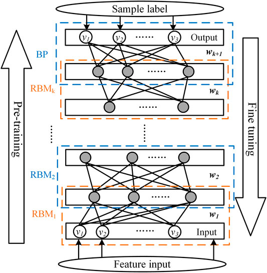
FIGURE 1. Structure of the DBN.

When all RMBs are fully trained, a layer of the BP classifier is added to the top layer to output the classification results. In this study, the classification error is measured by the cross-entropy loss function. The mini-batch stochastic gradient descent is used to supervise and fine-tune the parameters of the whole DBN. The adjustment amount of each backpropagation depends on the value of the loss function and the learning rate in the fine-tuning stage.

Cost-Sensitive Model Based on Fault Severity

In the power system, the misclassification costs of stable samples and unstable samples are obviously different. In addition, the impact of each training sample on the evaluation rules is also different. Therefore, a cost-sensitive method based on fault severity is proposed in this study.

Cost-Sensitive Method

The weight of the sample is changed, and one class is given a higher weight by the cost-sensitive method. In this way, the fitting degree of the evaluation model to the mentioned class is improved. For the machine learning–based model, the misclassification in the training process can correct the model. In general, the weight coefficients of all samples of the evaluation model are equal. For a binary classification problem, the cross-entropy function (Chen and Wang, 2021) is usually used as the loss function, as shown in Equation 1.

$L_i=-g^{\left(i\right)}\log g{\text{'}}^{\left(i\right)}-\left(1-g^{\left(i\right)}\right)\log \left(1-g{\text{'}}^{\left(i\right)}\right),(1)$

where $g^{\left(i\right)}$ is the true label of the ith sample; $g{\text{'}}^{\left(i\right)}$ is the predicted label of the ith sample.

The prediction accuracy of each sample is considered by the cross-entropy function. If the model is of low accuracy, the model will give a larger loss value to strengthen the learning of samples; otherwise, a smaller loss value is given. However, when the numbers and misclassification costs of various types are different, the traditional cross-entropy function is no longer applicable. Hence, a cost-sensitive method is introduced.

A weight coefficient is introduced in the cost-sensitive method on the basis of (1) so that the calculation of the loss function is biased toward the expected direction. In power system application, the weight coefficient of unstable samples is increased to make the evaluation rules tend toward unstable samples, thereby improving the accuracy of unstable samples. The loss function combined with the cost-sensitive method is modified as (2).

${L^{\prime }}_i=-g^{\left(i\right)}\log g{\text{'}}^{\left(i\right)}-\alpha \left(1-g^{\left(i\right)}\right)\log \left(1-g{\text{'}}^{\left(i\right)}\right),(2)$

where $\alpha$ is the misclassification cost coefficient of unstable samples. The larger the value of $\alpha$ is, the better the model fits the unstable samples and the higher the accuracy of unstable samples.

Cost-Sensitive Method Based on Fault Severity

In this work, the relative clearing time is used as a measure of fault severity. The fault severity x_i of each unstable sample is calculated by (3). The smaller the absolute value of x_i, the closer the sample is to the critical state.

$x_i=\frac{t_L-t_i}{t_L},(3)$

where x_i represents the fault severity of the ith sample; t_i represents the fault duration of the ith sample; and t_L represents the fault critical clearing time of the ith sample.

In the power system, fault samples can be divided into critical samples and noncritical samples according to fault severity. Since critical samples and noncritical samples have different influences on the evaluation rules, the influence degree of the two should be compared. The loss function can be used to measure the difference between the predicted value and true value. It can quantify the sample fitting situation and reflect the evaluation performance of the model. The model parameters are modified based on the loss function to improve the sample fitting degree in the training process. Therefore, the ratio of the mean loss of critical samples and noncritical samples is calculated. Then, the influence of the critical samples and the noncritical samples on the evaluation rule can be compared.

The influence difference of critical samples and noncritical samples on evaluation rules is not considered in the traditional cost-sensitive method. The traditional cost-sensitive method treats the two types in the same way and assigns them equal weights. For critical samples are more easily to be misjudged than noncritical samples, critical samples should be assigned a larger weight. In this way, the model will pay more attention to the loss value of critical samples and improve the accuracy of critical samples. Therefore, a cost-sensitive method based on fault severity is proposed in this study. Different weights of critical samples and noncritical samples are assigned so that the cost coefficient of critical samples is increased and that of noncritical samples is reduced at the same time. By this method, the evaluation model focuses on the judgment of critical samples and improves the rationality of cost-sensitive assignments, thereby improving the global accuracy of the model.

Firstly, the fault severity x_i of each unstable sample is calculated; then, according to the fault severity x_i, weight coefficient ${\beta }_i$ is assigned to each sample. A linear or nonlinear function can be used as the cost function, as long as the weight coefficient of critical samples is higher than that of noncritical samples in the cost function. The simplest and clearest linear function as shown in Equation 5 is utilized in this study to prove the feasibility of the proposed method. The loss function of the ith sample is expressed as (4).

${L^{″}}_i=-g^{\left(i\right)}\log g{\text{'}}^{\left(i\right)}-{\beta }_i\left(1-g^{\left(i\right)}\right)\log \left(1-g{\text{'}}^{\left(i\right)}\right),(4)$

${\beta }_i=\left(x_i+\mathrm{k}\right)\times \mathrm{b,}(5)$

where b is the adjustment coefficient, which determines the slope of the cost coefficient of the unstable samples; k is any positive real number; and k and b jointly determine the maximum value of the cost coefficient of the unstable samples.

Taking the fault severity as the abscissa and the cost coefficient as the ordinate, Figure 2 shows the assignment method of the cost coefficient based on fault severity.

FIGURE 2

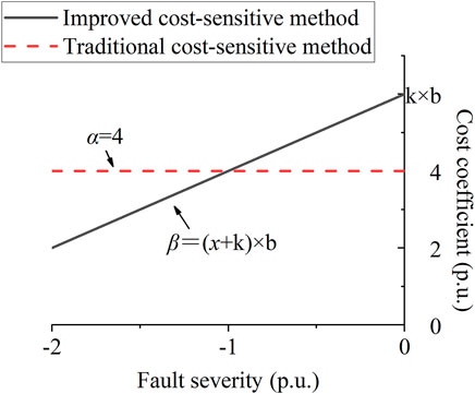
FIGURE 2. Cost sample based on fault severity.

The improved cost-sensitive method linearizes the cost coefficient of unstable samples. The closer unstable samples to the critical situation, the higher the cost coefficient. Compared with traditional cost-sensitive methods, the proposed method assigns lower cost coefficients to noncritical samples and higher cost coefficients to critical samples so that the evaluation rules are more reasonable.

Transient Stability Assessment Model

The construction of the DBN-based TSA model includes feature extraction, sample labeling, model training, and performance evaluation. Specific steps are as follows.

(Ⅰ) Feature extraction: four important moments (the moment before the fault occurs, the moment when the fault occurs, the moment when the fault is cleared, and the moment after the fault is cleared) are selected as the feature extraction time step. The power angle, angular velocity, active power, and reactive power of each generator of the four moments are extracted.

(Ⅱ) Sample labeling: The transient stability state of samples is determined according to the maximum power angle difference of any two generators. (6) is used to determine whether the sample is stable.

$\phi =\mathrm{36}{\mathrm{0}}^{\text{o}}-|\Delta {\delta }_{\max }|.(6)$

If φ ≤ 0, the sample is stable and the label is 1; if φ > 0, it is unstable and the label is 0.

(Ⅲ) Model training: Unsupervised pre-training and supervised fine-tuning are adopted. Unsupervised pre-training can make the model search for a better initial value; supervised fine-tuning can ensure that the trained model matches the real evaluation rules.

(Ⅳ) Performance evaluation: The test set is utilized to test the performance of the DBN after training. The evaluation indexes are the recall rate R₀ of unstable samples, the recall rate R₁ of stable samples, and the whole accuracy rate A of all samples. Those evaluation indexes are defined as follows.

$R_0=\frac{TN}{TN+FP},(7)$

where TN is the number of unstable samples accurately predicted; FP is the number of unstable samples mispredicted.

$R_1=\frac{TP}{TP+FN},(8)$

where TP is the number of stable samples accurately predicted; FN is the number of stable samples mispredicted.

$A=\frac{TP+TN}{TP+FP+TN+FN}.(9)$

Case Study

The IEEE 39-bus system is adopted as the test system; its topology is shown in Figure 3 (Ma et al., 2021; Zhang et al., 2019). The system frequency is 60 Hz. The simulation software PSD-BPA of Chinese Academy of Electric Power Sciences is adopted for time-domain simulation. The load level of the IEEE39-bus system is 90, 95, 100, 105, and 110%. Three-phase short-circuit faults are set at 10, 50, and 90% of each transmission line length. The system frequency is 60 Hz. The fault duration is 6–18 cycles. A simulation test is carried out every half cycle, a total of 25 types. 12,375 kinds of fault conditions are randomly simulated by PSD-BPA. 4,374 samples are randomly selected as the training set and 2000 as the test set. The ratio of unstable samples and stable samples is 1: 1 in the training set and test set.

FIGURE 3

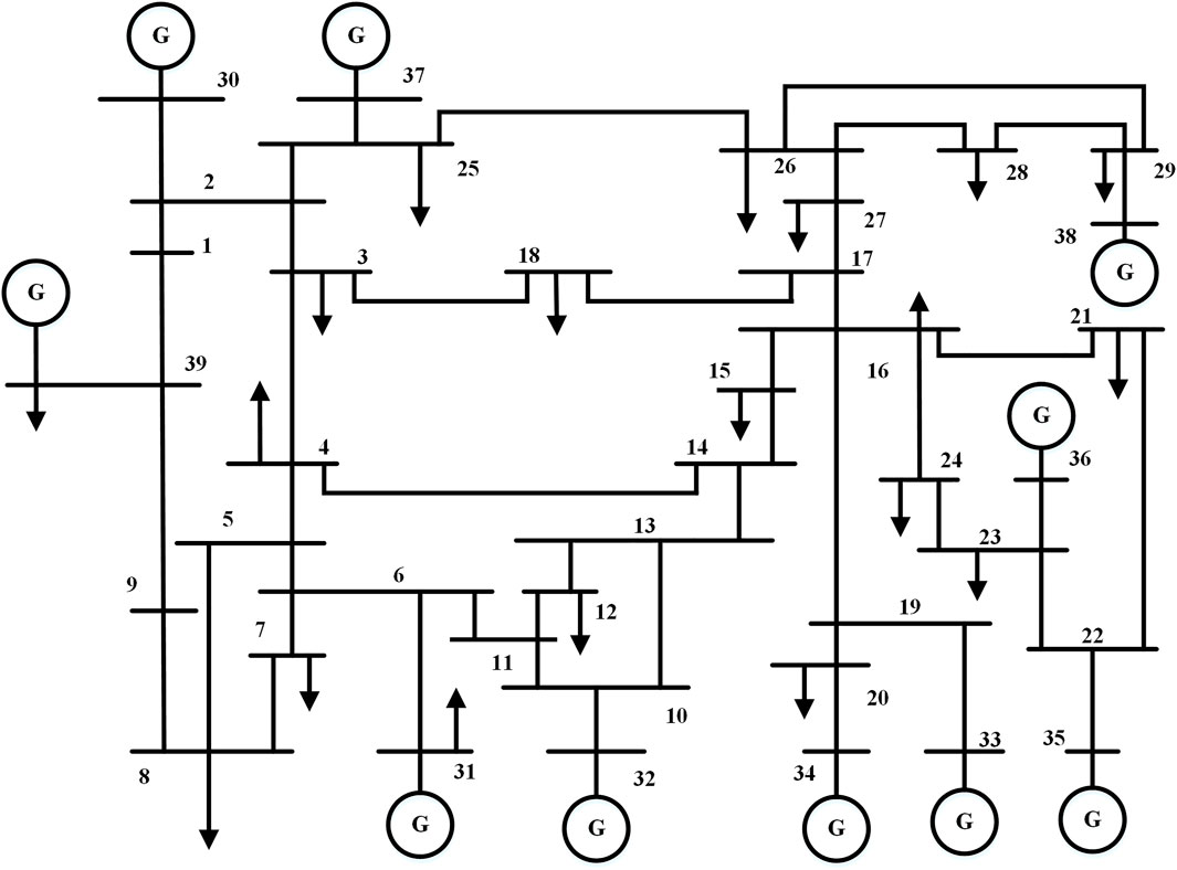
FIGURE 3. Structure of the IEEE 39-bus system.

Performance Analysis of the DBN Model

To verify the effectiveness of the DBN, it is compared with two commonly used machine learning algorithms, support vector machine (SVM) (You et al., 2013) and decision tree (DT) (Zhang et al., 2019). In this study, the five-fold cross-validation is applied to select DBN parameters. Finally, the learning rate in the pre-training stage of the DBN is 0.5, and the learning rate in the fine-tuning stage is 0.2. The number of neurons in each hidden layer is 256, 128, 64, and 32. The number of training times is 100. SVM uses radial basis function as the kernel function. DT uses the CART algorithm. Five training sets are randomly simulated, and the average of the five results is used as the final result, as shown in Table 1.

TABLE 1

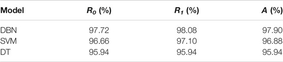
TABLE 1. Accuracy of different models.

It is shown in Table 1 that the whole accuracy of DBN, SVM, and DT all can reach more than 95%. The evaluation indexes R₀, R₁, and A are higher than those of other models. DBN has powerful feature extraction capabilities and its deep architecture can abstract deep features layer by layer so that it can improve the evaluation accuracy. Compared with other shallow learning methods, DBN has better evaluation performance.

Effectiveness of the Improved Cost-Sensitive Method

In this part, the improved cost-sensitive method is compared with the original data and traditional cost-sensitive methods to verify the feasibility of the proposed method. The cost coefficients of the unstable samples of the improved cost-sensitive method b, k are taken as 3 and 3, respectively; the cost coefficients of the unstable samples of the traditional cost-sensitive method α are taken as 3, 6, and 9.

Figure 4 shows the cost-sensitive assignment of five models to unstable samples.

FIGURE 4

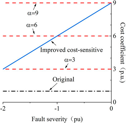
FIGURE 4. Unstable sample cost-sensitive assignment method of different models.

To overcome the interference caused by the randomness of the data, the training set and the test set are randomly sampled five times, and the average of the five experimental results of the test set is taken as the final result. The three evaluation indexes R₀, R₁, and A of each method are calculated to reflect the model performance. The results are shown in Table 2. The number of samples is taken as the horizontal axis, and each evaluation index is taken as the vertical axis to show the results in Figure 5–7.

TABLE 2

TABLE 2. Evaluation results of different models.

FIGURE 5

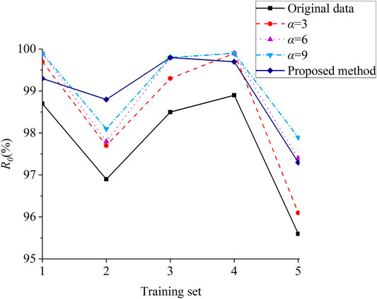
FIGURE 5. Accuracy of test set unstable samples.

FIGURE 6

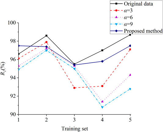
FIGURE 6. Accuracy of test set stable samples.

FIGURE 7

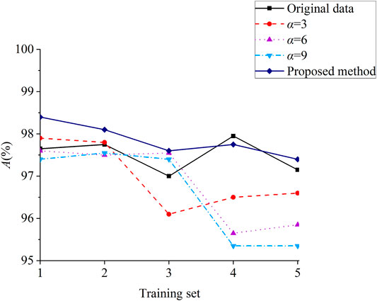
FIGURE 7. Global accuracy of test set samples.

It can be seen from the results that compared with the original data, the traditional cost-sensitive method has a certain improvement in the evaluation accuracy of unstable samples. However, the evaluation accuracy of stable samples is reduced more. This is because traditional cost-sensitive samples pay more attention to unstable samples. Though the fitting degree of unstable samples is significantly improved, and the results tend to be judged as unstable, the evaluation accuracy of stable samples is greatly reduced. Moreover, the whole accuracy of the TSA model is also decreased. With the increase of α in the traditional cost-sensitive method, the whole accuracy of the method is decreased accordingly.

According to different fault severities, different weight values are assigned by the improved cost-sensitive method. This improved method ensures that the model performance is better than that of the traditional cost-sensitive method. Compared with the original data, the accuracy of unstable samples is significantly improved while the accuracy of stable samples is not decreased greatly. Of course, the proposed method performs best in whole accuracy with 97.85%. Compared with the traditional cost-sensitive method (α = 3, α = 6), the accuracy of unstable samples and stable samples is higher in the proposed method. Compared with the method with higher cost-sensitive value (α = 9), the accuracy of unstable samples is not much different, while the accuracy of stable samples of the proposed method is greatly improved.

Real-Time Performance of the Improved Cost-Sensitive Method

In order to illustrate the real-time performance of the improved cost-sensitive method, the simulation time is calculated. A computer with i7-9750H 2.6 GHz CPU and 16 GB RAM is applied for simulation. The training time is 100. The simulation time is shown in Table 3.

TABLE 3

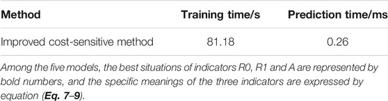
TABLE 3. Simulation time of the proposed method.

It can be seen from Table 3 that the training time of the improved cost-sensitive method is 81.18s, while the prediction time of a sample is only 0.26 ms. For the deep learning–based TSA, the training process is carried out offline, so it can be allowed a long training time. At the same time, due to short prediction time, sufficient time is reserved for the implementation of the next control measures. In addition, with the improvement of computer performance, the evaluation performance of the proposed model will be further improved. Consequently, the proposed method can meet the requirements of real time.

Conclusion

A cost coefficient assignment method based on fault severity is proposed in this study. By this method, the fault severity of each unstable sample is calculated according to the fault duration time. Different weights are assigned to samples with different fault severities. The closer to the critical situation, the greater the weight value is. This assignment method takes full account of the different impacts of critical samples and noncritical samples on the evaluation model. Moreover, the recognition of critical samples is improved by the proposed method. At the same time, the interference of noncritical samples to the evaluation rules is reduced, making the rules more reasonable. DBN is taken as an example to carry out simulation tests.

Combined with the proposed cost-sensitive method, the DBN-based TSA model can achieve the optimization of the evaluation results. Compared with traditional cost-sensitive methods, the proposed method not only retains the high fitting degree of unstable samples but also improves the evaluation accuracy of stable samples and whole accuracy. Therefore, in the power system, the improved cost-sensitive method can enable the machine learning–based TSA model to be better applied to transient stability.

Data Availability Statement

The original contributions presented in the study are included in the article/Supplementary Materials; further inquiries can be directed to the corresponding author.

Author Contributions

JL: conceptualization, methodology, writing–review and editing, and supervision. RC: software and writing–original draft. ZZ: writing–revised manuscript.

Funding

The study was supported by Reform of the Four-in-One Three-dimensional Electrical Application-Oriented Talent Training Mode for New Engineering project (grant agreement number FBJG20190204).

Conflict of Interest

The authors declare that the research was conducted in the absence of any commercial or financial relationships that could be construed as a potential conflict of interest.

Publisher’s Note

All claims expressed in this article are solely those of the authors and do not necessarily represent those of their affiliated organizations, or those of the publisher, the editors, and the reviewers. Any product that may be evaluated in this article, or claim that may be made by its manufacturer, is not guaranteed or endorsed by the publisher.

Abbreviation

DBN, deep belief network; DT, decision tree; BP, backpropagation; RBM, restricted Boltzmann machine; SVM, support vector machine; TSA, transient stability assessment.

References

Chang, H., Chu, C., and Cauley, G. (1995). Direct Stability Analysis of Electric Power Systems Using Energy Functions: Theory, Applications, and Perspective. Proc. IEEE 83 (11), 1497–1529. doi:10.1109/5.481632

CrossRef Full Text | Google Scholar

Chen, Q., Lin, N., and Wang, H. (2021). Transient Stability Assessment Model with Parallel Structure and Data Augmentation. Int. Trans. Electr. Energ. Syst. 31 (5), e12872. doi:10.1002/2050-7038.12872

CrossRef Full Text | Google Scholar

Chen, Q., and Wang, H. (2021). Time-adaptive Transient Stability Assessment Based on Gated Recurrent Unit. Int. J. Electr. Power Energ. Syst. 133, 107156. doi:10.1016/j.ijepes.2021.107156

CrossRef Full Text | Google Scholar

Chen, Z., Xiao, X., Li, C., Zhang, Y., and Hu, Q. (2016). Real-time Transient Stability Status Prediction Using Cost-Sensitive Extreme Learning Machine. Neural Comput. Applic 27 (2), 321–331. doi:10.1007/s00521-015-1909-9

CrossRef Full Text | Google Scholar

Han, T., Chen, Y., Ma, J., Zhao, Y., and Chi, Y.-y. (2018). Surrogate Modeling-Based Multi-Objective Dynamic VAR Planning Considering Short-Term Voltage Stability and Transient Stability. IEEE Trans. Power Syst. 33 (1), 622–633. doi:10.1109/tpwrs.2017.2696021

CrossRef Full Text | Google Scholar

Han, T., Chen, Y., and Ma, J. (2018). Multi-objective Robust Dynamic VAR Planning in Power Transmission Girds for Improving Short-Term Voltage Stability under Uncertainties. IET Generation, Transm. Distribution 12 (8), 1929–1940. doi:10.1049/iet-gtd.2017.1521

CrossRef Full Text | Google Scholar

Hiskens, I. A., and Hill, D. J. (1989). Energy Functions, Transient Stability and Voltage Behaviour in Power Systems with Nonlinear Loads. IEEE Trans. Power Syst. 4 (4), 1525–1533. doi:10.1109/59.41705

CrossRef Full Text | Google Scholar

Hou, J., Xie, C., Wang, T., Yu, Z., Lu, Y., and Dai, H. (2018). “Power System Transient Stability Assessment Based on Voltage Phasor and Convolution Neural Network,” in Proceeding of the the 2018 IEEE International Conference on Energy Internet (ICEI), Beijing, China, May 2018 (IEEE), 247–251.

CrossRef Full Text | Google Scholar

Hu, X., Zhang, H., Ma, D., and Wang, R. (2021). A tnGAN-Based Leak Detection Method for Pipeline Network Considering Incomplete Sensor Data. IEEE Trans. Instrumentation Meas. 70, 3510610. doi:10.1109/tim.2020.3045843

CrossRef Full Text | Google Scholar

Hu, X., Zhang, H., Ma, D., and Wang, R. (2021). Hierarchical Pressure Data Recovery for Pipeline Network via Generative Adversarial Networks. IEEE Trans. Automat. Sci. Eng., 1–11. doi:10.1109/TASE.2021.3069003

CrossRef Full Text | Google Scholar

Li, X., Yang, Z., Guo, P., and Cheng, J. (2021). An Intelligent Transient Stability Assessment Framework with Continual Learning Ability. IEEE Trans. Ind. Inf. 17 (12), 8131–8141. doi:10.1109/tii.2021.3064052

CrossRef Full Text | Google Scholar

Ma, D., Hu, X., Zhang, H., Sun, Q., and Xie, X. (2021). A Hierarchical Event Detection Method Based on Spectral Theory of Multidimensional Matrix for Power System. IEEE Trans. Syst. Man. Cybern, Syst. 51 (4), 2173–2186. doi:10.1109/tsmc.2019.2931316

CrossRef Full Text | Google Scholar

Mahdi, M., and Genc, V. M. I. (2018). Post-fault Prediction of Transient Instabilities Using Stacked Sparse Autoencoder. Electric Power Syst. Res. 164, 243–252. doi:10.1016/j.epsr.2018.08.009

CrossRef Full Text | Google Scholar

Sobajic, D. J., and Pao, Y.-H. (1989). Artificial Neural-Net Based Dynamic Security Assessment for Electric Power Systems. IEEE Trans. Power Syst. 4 (1), 220–228. doi:10.1109/59.32481

CrossRef Full Text | Google Scholar

Tan, B., Yang, J., Tang, Y., Jiang, S., Xie, P., and Yuan, W. (2019). A Deep Imbalanced Learning Framework for Transient Stability Assessment of Power System. IEEE Access 7, 81759–81769. doi:10.1109/access.2019.2923799

CrossRef Full Text | Google Scholar

Tang, C. K., Graham, C. E., El-Kady, M., and Alden, R. T. H. (1994). Transient Stability index from Conventional Time Domain Simulation. IEEE Trans. Power Syst. 9 (3), 1524–1530. doi:10.1109/59.336108

CrossRef Full Text | Google Scholar

Wang, H., and Wang, Q. (2022). Adaptive Cost-Sensitive Assignment Method for Power System Transient Stability Assessment. Int. J. Electr. Power Energ. Syst. 135, e107574. doi:10.1016/j.ijepes.2021.107574

CrossRef Full Text | Google Scholar

Wang, H., Wang, Q., and Chen, Q. (2020). Transient Stability Assessment Model with Improved Cost-Sensitive Method Based on the Fault Severity. IET Generation, Transm. Distribution 14 (20), 4605–4611. doi:10.1049/iet-gtd.2020.0967

CrossRef Full Text | Google Scholar

Wang, H., Chen, Q., and Zhang, B. (2020). Transient Stability Assessment Combined Model Framework Based on Cost-Sensitive Method. IET Generation, Transm. Distribution 14 (12), 2256–2262. doi:10.1049/iet-gtd.2019.1562

CrossRef Full Text | Google Scholar

Xue, Y. (1998). “Fast Analysis of Stability Using Eeac and Simulation Technologies,” in POWERCON '98. 1998 International Conference on Power System Technology. Proceedings (Cat. No.98EX151), Beijing, China, Aug. 1998 (IEEE), 12–16.

Google Scholar

Yan, R., -Masood, N.-A., Kumar Saha, T., Bai, F., and Gu, H. (2018). The Anatomy of the 2016 South australia Blackout: a Catastrophic Event in a High Renewable Network. IEEE Trans. Power Syst. 33 (5), 5374–5388. doi:10.1109/tpwrs.2018.2820150

CrossRef Full Text | Google Scholar

Yan, R., Geng, G., Jiang, Q., and Li, Y. (2019). Fast Transient Stability Batch Assessment Using Cascaded Convolutional Neural Networks. IEEE Trans. Power Syst. 34 (4), 2802–2813. doi:10.1109/tpwrs.2019.2895592

CrossRef Full Text | Google Scholar

You, D., Wang, K., Ye, L., Wu, J., and Huang, R. (2013). Transient Stability Assessment of Power System Using Support Vector Machine with Generator Combinatorial Trajectories Inputs. Int. J. Electr. Power Energ. Syst. 44 (1), 318–325. doi:10.1016/j.ijepes.2012.07.057

CrossRef Full Text | Google Scholar

Yu, J. J. Q., Hill, D. J., Lam, A. Y. S., Gu, J., and Li, V. O. K. (2018). Intelligent Time-Adaptive Transient Stability Assessment System. IEEE Trans. Power Syst. 33 (1), 1049–1058. doi:10.1109/tpwrs.2017.2707501

CrossRef Full Text | Google Scholar

Zadkhast, S., Jatskevich, J., and Vaahedi, E. (2015). A Multi-Decomposition Approach for Accelerated Time-Domain Simulation of Transient Stability Problems. IEEE Trans. Power Syst. 30 (5), 2301–2311. doi:10.1109/tpwrs.2014.2361529

CrossRef Full Text | Google Scholar

Zhang, Y., Xu, Y., and Dong, Z. Y. (2018). Robust Ensemble Data Analytics for Incomplete Pmu Measurements-Based Power System Stability Assessment. IEEE Trans. Power Syst. 33 (1), 1124–1126. doi:10.1109/tpwrs.2017.2698239

CrossRef Full Text | Google Scholar

Zhang, Y., Xu, Y., Bu, S., Dong, Z. Y., and Zhang, R. (2019). Online Power System Dynamic Security Assessment with Incomplete PMU Measurements: a Robust white-box Model. IET Generation, Transm. Distribution 13 (5), 662–668. doi:10.1049/iet-gtd.2018.6241

CrossRef Full Text | Google Scholar

Zheng, L., Hu, W., Zhou, Y., Min, Y., Xu, X., Wang, C., et al. (2017). “Deep Belief Network Based Nonlinear Representation Learning for Transient Stability Assessment,” in Power and Energy Society General Meeting, 1–5. doi:10.1109/pesgm.2017.8274126

CrossRef Full Text | Google Scholar

Zhou, Y., Guo, Q., Sun, H., Yu, Z., Wu, J., and Hao, L. (2019). A Novel Data-Driven Approach for Transient Stability Prediction of Power Systems Considering the Operational Variability. Int. J. Electr. Power Energ. Syst. 107, 379–394. doi:10.1016/j.ijepes.2018.11.031

CrossRef Full Text | Google Scholar

Zhu, L., Lu, C., Dong, Z. Y., and Hong, C. (2017). Imbalance Learning Machine-Based Power System Short-Term Voltage Stability Assessment. IEEE Trans. Ind. Inf. 13 (5), 2533–2543. doi:10.1109/tii.2017.2696534

CrossRef Full Text | Google Scholar