Characteristic of Steady-State Flow Force on the Cone Valve Based on Orthogonal Test Method

The steady-state flow force is the fundamental reason that affects the pressure stability, which will reduce the control performance of a hydraulic valve. A mathematical model of the axial steady-state flow force on the valve core is proposed to master the principle and characteristics of steady-state flow force. For understanding the dynamic changes of the steady-state flow force, a two-dimensional axisymmetric model is built to discuss the value of flow force. Different geometric parameters and operating conditions have different effects on the performance of the valve, and analyzing a variety of parameters is difficult because of the complexity of the test. Therefore, the geometric parameters and operating conditions in the steady-state flow force were optimized by the orthogonal test-optimization method. The main significant factors affecting the performance of steady-state flow force on the cone valve core are determined by extreme difference analysis, which are the opening and pressure differential, respectively. Furthermore, a test ring is built to measure the steady-state flow force. The results show that the greater the pressure differential is, the greater the steady-state flow force is. The steady-state flow force does not increase linearly, but increases first and then decreases with the increase of the opening. The study will lay the foundation to precise axial flow force prediction and reference for design optimization of the valve.

Introduction

Cone valve is the main control component of the hydraulic systems, which is widely used due to their advantages of fast dynamic response, high control accuracy, and simple structure. The flow force is one of the most important reasons for the vibration of the cone valve, which has a significant influence on the stability and accuracy of the hydraulic system (Li et al., 2018). In the working process of the cone valve, the flow force will impede the spool displacement, cause the vibration of the cone valve, and reduce the reliability of valve, so far as to shorten the service life of the cone valve. A comprehensive understanding of the flow force is rather complicated, which is closely related to complex flow fields in the valve. Due to the complex flow channel structure of the valve, there may be complex turbulence phenomenon. Because of this complexity and uncertainty in the turbulence flow, it is difficult to effectively estimate the precise information caused by the flow force. Therefore, it is very necessary to fully investigate the reason, influencing factors, and variation characteristics of flow force in conical valve, which is of great significance to improve the control performance of the hydraulic system.

Many scholars have carried out the research on the flow field characteristics of the valve and deepened the research on the flow force (Kang et al., 2020). Jia et al. (2019) studied the fluctuation of the pressure in the cone valve to obtain the L/D parameter, which had the greatest impact on the stability of the system and could be used to predict the more stable flow force output of the system. Gao et al. (2019) took the influence of flow force into account and developed a nonlinear mathematical model to improve the valve’s performance. Han et al. (2017) investigated unsteady cavitation process inside a water hydraulic poppet valve, and pointed that the flow force will increase with the increase of cone angles, and cavitation could slightly decrease the flow force. Zong et al. (2020) got the steady-state flow forces exerted on the valve disk at different valve openings numerically and experimentally. However, it is hard to get how flow force works on different types of valves because of the turbulent flow in the valve. Lei et al. (2018) discussed the flow model of the poppet valve orifice with a novel function of flow discharge coefficient, and the flow force caused by the valve body motion and the flowrate variation are also considered; CFD method (Computational Fluid Dynamics) and experimental evaluation are combined together, predicting the flow force more accurately. Zhang et al. (2019) studied the opening characteristics of the dynamic relief valve by combining numerical calculation and experimental research, and then obtained the correlation between operating parameters and variation characteristics of the flow force. Filo et al. (2019) proposed a new core head geometry to improve the valve’s performance by analyzing the flow force of differential switch valve installed in throttle check valve body. Tan et al. (2019) analyzed the force of the split proportion valve core numerically and got the influence of the valve core structure parameters on the force. Yang et al. (2019a, 2019b) compared and analyzed the continuous micro-jet control flapper nozzle pilot valves with traditional nozzle and micro-nozzle, then obtained the influence of different structural parameters on the flow force. Lin et al. (2018) presented a novel method to reduce the overflow loss using an energy recovery unit and pointed that the steady-state flow force decreases dramatically with increasing return line pressure. Scuro et al. (2018) pointed that average normal disc force is about 19% lower than theoretical ASME force, which could prevent the valve oversizing. Kang et al. (2020) pointed that the fluctuation of the flow force of the pilot stage will affect the output stability of the servo valve. However, most research focus on flow force in the slide valve rather than the cone valve, and a single control volume is used to calculate the flow force and the influence of wall surface is not considered. There are many factors affecting the flow force, such as opening, the inlet and outlet pressure, the cone angle of the conical valve core, the diameter of valve core, the radius of flow channel, and the density of the fluid, not only the geometric parameters but also operating conditions. Different parameters have different effects on the control accuracy of valve, so analyzing a variety of parameters on the flow force is difficult because of the complexity of the test. Although some literature discussed the effect of pressure differential and opening on the flow force, their findings were not comprehensive enough and did not apply the influence degree of each factor.

In this paper, a mathematical model of axial steady-state flow force based on the momentum theorem and Bernoulli equation is derived to perform a detailed force analysis of the control volume in the upstream and downstream flow channels of cone valve. A test ring is used to measure axial steady-state flow force at different conditions to validate the model. In addition, for the comprehensive consideration of geometric parameters and operating conditions, an orthogonal test combined with extreme difference analysis is used to examine factors affecting flow force. The weight between geometric parameters and operating conditions is discussed, and the most significant influence parameters on the flow force are presented. Then the value of flow force on the variation of pressure and opening of the cone valve are investigated. The paper will provide theoretical guidance for the calculation of flow force, give reference for design optimization, and control accuracy improvement of the valve.

Theoretical Analysis of Steady-State Flow Force

As shown in Figure 1A, the flow area of the internal flow cone valve is divided into two control volumes taking the orifice as the interface; the upper valve abcd-a′b′c′d′ is defined as control volume I, the lower valve efghijk is defined as control volume II, and the upward direction is used as the positive direction. The momentum theorem is applied to analyze the force in control bodies I and II, which are shown as follows:

$-m{v}_f-\left(-mv\sin \alpha \right)=-F_{\mathrm{{\rm I}}}+P_s\mathrm{\Delta }A(1)$

$-m{v}_2-\left(-m{v}_f\right)=-F_{\mathrm{{\rm I}}\mathrm{{\rm I}}}+P_2{A}_2(2)$

where m is the mass of fluid passing through flow section per unit time, $v_f$ is the velocity of fluid flowing through the orifice, $v$ is the velocity of fluid flowing into control volume I, α is the angle of horizontal velocity direction in the control volume I, F_II is the axial force acting on control volume I by valve core, Ps is the pressure on the ring ad-a′d′ at the valve seat in control volume I, ΔA is the area on the ring ad-a′d′in control volume I, v₂ is the velocity of fluid flowing out of the control volume II, F_Ⅱ is the axial force acting on control volume II by valve core, P₂ is the outlet pressure, and A₂ is the cross-sectional area of the downstream channel. Combined with Eqs 1, 2, the total axial force F_axis acting on control volume by valve core could be obtained, which is defined as follows:

$F_{axis}=F_{\mathrm{{\rm I}}}+F_{\mathrm{{\rm I}}\mathrm{{\rm I}}}(3)$

FIGURE 1

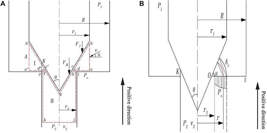
FIGURE 1. Schematic diagram of control valve: (A) control volume; (B) pressure distribution at the shoulder.

According to Newton’s third law of motion, action and reaction are equal and opposite. The force F on the cone valve core could be obtained, which is shown as

$F=-F_{axis}=\rho Qv\sin \alpha -\rho Q{v}_2-P_s\mathrm{\Delta }A-P_2{A}_2(4)$

where ρ is the fluid density and Q is the fluid flow. When the fluid flows into and out of control volume I, the velocity of fluid will change with the position of the flow area. According to the Bernoulli equation, the pressure of fluid from the inlet to the outlet will also change.

As shown in Figure 1B, the control volumes I and II have good symmetry. By using the axisymmetric theoretical model, we usually can get good effect in solving problems. Point O could be obtained by extending the line ad to intersect with the valve core, and then a few equally spaced nodes are set in the line ad to divide it into several smaller segments. Some different length segments could be obtained by connecting each node with the point O, and then the isobaric surfaces at different positions in the line ad could be obtained by drawing an arc with each small segment, which is the radius, and the point O, which is the center of the circle. Therefore, the PsΔA is defined as follows:

$P_s\mathrm{\Delta }A={\displaystyle {\int }_{r_2}^{r_1}2\pi r\left[P_1-\frac{\rho }{2}{\left(\frac{Q}{A_r}\right)}^2\right]}dr(5)$

$A_r=2\pi r\frac{\left(r-r_2+K\tan \theta \right)\cos \theta }{\cos \left(\frac{\pi }{4}-\frac{\theta }{2}\right)}(6)$

where r₁ is the radius of valve core, r₂ is the radius of the flow channel downstream, P₁ is the inlet pressure, A_r is the area of isobaric surface, K is the opening of the valve core, and θ is the half cone angle of the valve core.

Combining Eqs. 4–6, the hydrostatic pressure F_P could be obtained. The mathematical model of the axial steady-state flow force on the internal flow cone valve core is listed as follows:

$F_s=\rho Qv\sin \alpha -\rho Q{v}_2-{\displaystyle {\int }_{r_2}^{r_1}2\pi r{P}_s}dr-P_2{A}_2-F_p(7)$

As shown in Eq. 7, the axial steady-state flow force is not only influenced by geometric parameters but also influenced by operating conditions, such as opening, inlet and outlet pressure, the angle and radius of the valve core, the radius of the flow channel downstream, and the density of the fluid. While other physical conditions all remain unchanged except the opening, the axial steady-state flow force does not simply change linearly with the increase of the opening. In fact, it is a nonlinear process.

Numerical Modelling

Governing Equations and Boundary Conditions

Continuity equation for the mixture is

$\frac{\partial }{\partial t}\left({\rho }_m\right)+\nabla \left({\rho }_m{\overrightarrow{\nu }}_m\right)=0(8)$

The momentum equation for the mixture is

$\frac{\partial }{\partial t}\left({\rho }_m{\overrightarrow{\nu }}_m\right)+\nabla \cdot \left({\rho }_m{\overrightarrow{\nu }}_m{\overrightarrow{\nu }}_m\right)=-\nabla p+\nabla \cdot \left[{\mu }_m\left(\nabla {\overrightarrow{\nu }}_m+\nabla {\overrightarrow{\nu }}_m^T\right)\right](9)$

The net mass transfer from liquid to vapor is often described by Schnerr and Sauer model:

$\frac{\partial }{\partial t}\left(\alpha {\rho }_{\nu }\right)+\nabla \cdot \left(\alpha {\rho }_{\nu }\overrightarrow{\nu }\right)=\frac{{\rho }_v{\rho }_l}{{\rho }_m}\frac{D\alpha }{Dt}(10)$

Here,

$R_e=\frac{{\rho }_l{\rho }_v}{{\rho }_m}\alpha \left(1-\alpha \right)\frac{3}{R_B}{\left(\frac{2}{3}\frac{P_v-P}{{\rho }_l}\right)}^{1/2};P\le P_v(11)$

$R_c=\frac{{\rho }_l{\rho }_v}{{\rho }_m}\alpha \left(1-\alpha \right)\frac{3}{R_B}{\left(\frac{2}{3}\frac{P-P_v}{{\rho }_l}\right)}^{1/2};P\ge P_v(12)$

where ρ_m is the mixture density; α_v is the vapor volume fraction; ${\overrightarrow{\nu }}_m$ and μ_m are the velocity and viscosity of the mixture, respectively; and R_e and R_C are the mass transfer between the vapor and liquid phases in cavitation.

The internal fluid’s flow state is turbulent because the Reynolds number in the cone valve is much greater than the critical Reynolds number. Based on the results of Park and Rhee (2012) and Lain et al. (2002), the RNG k–ε model in turbulent flow is used to study the flow force, which is shown as follows:

$\frac{\partial }{\partial t}\left(\rho k\right)+\frac{\partial }{\partial x_i}\left(\rho k{u}_i\right)=\frac{\partial }{\partial x_j}\left({\alpha }_k{\mu }_{eff}\frac{\partial k}{\partial x_j}\right)+G_k-\rho \epsilon +S_k(13)$

$\frac{\partial }{\partial t}\left(\rho \epsilon \right)+\frac{\partial }{\partial x_i}\left(\rho \epsilon u_i\right)=\frac{\partial }{\partial x_j}\left({\alpha }_{\epsilon }{u}_{eff}\frac{\partial \epsilon }{\partial x_j}\right)+\frac{C_{1\epsilon }}{k}\epsilon G_k-C_{2\epsilon }\rho \frac{{\epsilon }^2}{k}-R_{\epsilon }+S_{\epsilon }(14)$

where $G_k$ is the generation of turbulence kinetic energy due to the mean velocity gradients and ε is the fluid’s turbulent dissipation rate. σ_k and σ_ε are the turbulent Prandtl numbers for k and ε, respectively. C_1ε, C_2ε, and C_3ε are constants. S_k and S_ε are user-defined source terms.

The inlet and the outlet pressure are chosen as the boundary conditions in this paper. No.46 antiwear hydraulic oil is used for the hydraulic fluid, whose density is 889 kg/m³ and viscosity is 4.6 × 10⁻⁵ m²/s. In CFD simulation, according to the study of Han et al. (2017), the force could be expressed as follows:

$F_s=F_p-F_{x-axis}=F_p-{\displaystyle \int P_{dynamics}}{S}_c(15)$

where F_s is the flow force acting on the cone, F_p is the force that generated by the static pressure, P_dynamics is the dynamics pressure distributed on the surface of the spool, and S_c is the axial area of the conical surface.

Geometry and Mesh of the Cone Valve

Considering the axisymmetric structure of the valve, the computational domain could be simplified to a two-dimensional axisymmetric geometric model (Liang et al., 2016; Han et al., 2017). To save calculation time and reduce the complexity of numerical simulation, a two-dimensional axisymmetric model is adopted, as shown in Figure 2. The flow channel in the cone valve is divided into four regions. The structural grid is used in regions ⅰ, ⅱ, and ⅳ, while the unstructured grid and local encryption are used in region ⅲ because the flow field is complex due to the large variation of fluid velocities and pressures at the orifice. $R$ is the radius of the flow channel upstream and $L$ is the total length of flow channel.

FIGURE 2

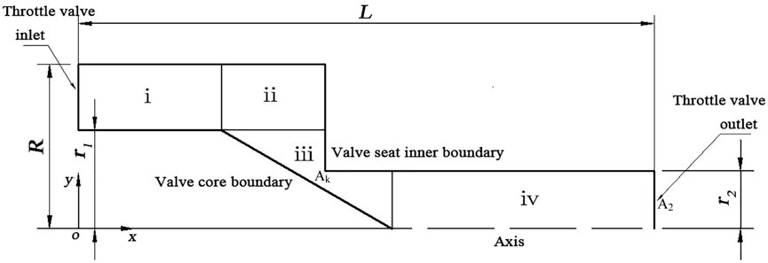
FIGURE 2. Geometric structure of the cone valve.

Figure 3 is the grid independence verification in region ⅲ because of local encryption of the grid under the same operating conditions. It could be found that the grid size gradually reduced in region ⅲ, while the corresponding mass flow rate reduced first, and then increase later, and finally it remains stable. Therefore, the mesh size of 0.032 mm is chosen for the simulation, to maintain the calculation accuracy and save the calculation time. The detailed of meshing near the orifice and partial enlarged drawing are shown in Figure 4, and the final grid number of the whole flow channels is about 80,000.

FIGURE 3

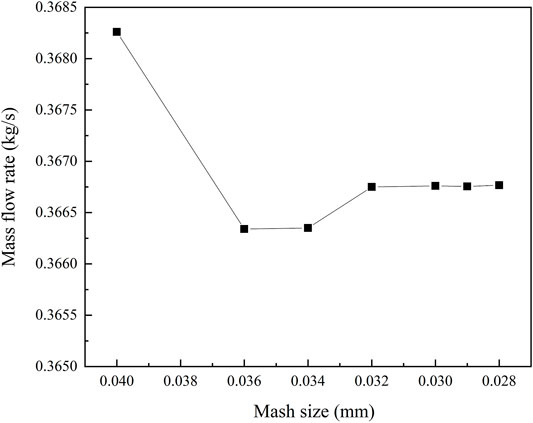
FIGURE 3. Verification of grid size independence at orifice.

FIGURE 4

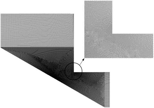
FIGURE 4. The detailed meshing.

Experimental Methods

Orthogonal Tests and Analyses

Different geometric parameters and operating conditions have different effects on the performance of steady-state flow force on the internal flow cone valve core, so analyzing their respective roles for flow force needs a tremendous amount of work. Therefore, the orthogonal test-optimization method is designed to study the combined effect of geometric parameters and operating conditions on the flow force. Table 1 shows the factors affecting the flow force and their levels. In this paper, four factors and four levels are selected for the orthogonal analysis of the flow force.

TABLE 1

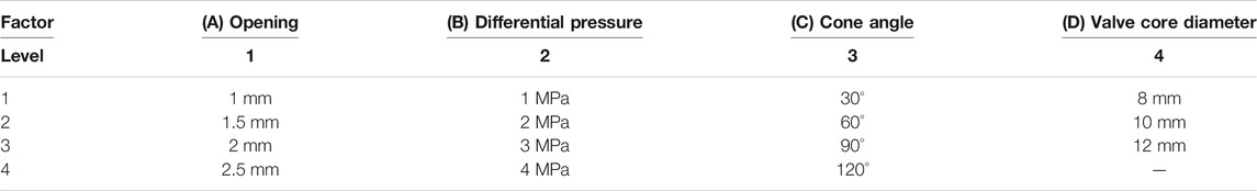
TABLE 1. Table of factor levels

According to the factor level numbers and data processing software SPSS, a suitable orthogonal test table $L_{19}\left(4^4\right)$ is developed and its header is also designed as shown in Table 2. The target of this analysis is to estimate the value of the flow force. According the test scheme shown in Table 2, a numerical simulation could be used to calculate the flow force (Xie et al., 2018), which is $F_s=F_{axis}-F_p$, $F_p=P_1{A}_1+P_2{A}_2=\pi (P_1+P_2)(r_1^2+r_2^2)$.

TABLE 2

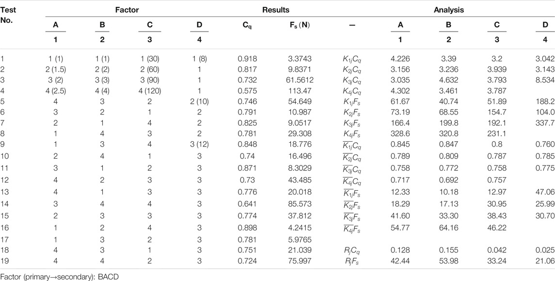
TABLE 2. Orthogonal test table

In Table 2, $K_{ij}$ is the sum of all test factors in column j and the level number i, ${\overline{K}}_{ij}$ is the average value of $K_{ij}$, and the optimal level and combination of factors in column j could be determined by the value of $K_{ij}$. $R_j$ is the extreme difference analysis of factor in column j, $R_j=\max \left\{{\overline{K}}_{ij}\right\}-\text{min}\left\{{\overline{K}}_{ij}\right\}$, which could reflect their variable range if there are fluctuations of the factors in column j. The larger $R_j$ is, the greater effect of this factor on this extreme difference analysis process is. According to the value of $R_j$, we could rank these factors in order of importance. It could been seen from the orthogonal test results in Table 2 that $R_2>R_1>R_3>R_4$. It points out some primary factors affecting the flow force and their important orders are pressure differential > opening > cone angle of valve core > the diameter of valve core. Therefore, these two factors, pressure differential and opening, have the most important influences on the flow force. This orthogonal test-optimization method provides a theoretical basis for the following flow force and its influencing factors.

Figure 5 shows the relationship between influencing factors and indicators, which helps us to better understand the influence of various factors on flow force at the unlimited and given level, so as to better assist the experimental work and save time. It could be found from Figure 5 that the flow force is the minimum when the opening reduces to the minimum $A_1$ and other conditions, such as the pressure differential, remain the same. When the pressure differential reduces to the minimum $B_1$ and other conditions, such as the opening, remain the same, the flow force is the minimum.

FIGURE 5

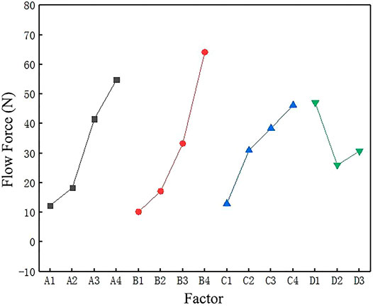
FIGURE 5. Comparison of experimental results of various factors.

Experimental System

The experimental device is shown in Figure 6, which consisted of a hydraulic system and a flow force measuring system. The hydraulic system contains a pump, an air-cooling device, an accumulator, a relief valve, a control valve, two flowmeters, a transparent test valve, a back throttle valve, two pressure gauges, and two pressure sensors. They are all connected by oil tubes. The hydraulic pump is used to provide power for this system. The air-cooling device is used to keep the oil at constant temperature, and the accumulator is used to reduce the pressure pulsation of this system. The relief valve, control valve, and back throttle valve are used to control the pressure and flow of the system. The inlet and outlet pressure of the transparent test valve are displayed by two pressure gauges. Two pressure sensors are used to monitor the inlet and outlet pressure of the test valve in real time. The flow force measuring system consisted of a displacement sensor and a micro-force sensor. The transparent valve is self-designed for installing this flow force measuring system. The opening of this test valve is measured by the displacement sensor, and the micro-force sensor is used to measure the flow force. The measured signals are collected and transmitted to the computer via a data acquisition card. All these components and parts are mounted on a self-designed optical platform to reduce vibration and improve the accuracy of the results.

FIGURE 6

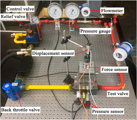
FIGURE 6. Experimental system.

Results and Discussion

As discussed in the aforementioned orthogonal tests, the pressure differential and the opening are the most important factors influencing the characteristics of steady-state flow force. The relationship between the pressure differential, the opening, and steady-state flow force is discussed theoretically, numerically, and experimentally in this section.

Effects of Pressure on Steady-State Flow Force Characteristics of the Valve

Figure 7 shows the relationship among the $A_k$, $A_2$ and the valve core’s opening $K$. The cross-sectional area $A_k$ of the cone valve orifice is defined in Figure 2, which is the minimum flow area. $A_2$ is defined as the maximum area $A_{max}$ (Ye et al., 2014) when $K_{max}$ is 5 mm. It could be seen that $A_k$ increases with the increasing opening of the valve, while the opening is less than 5 mm.$A_k$ is equal to the area of the channel downstream A₂ while k = 5 mm. If the opening continues to increase, A₂ will be smaller than $A_k$, and the throttling effect of the cone valve will disappear. Therefore, the range of the opening in this paper varies from 0 to 5 mm.

FIGURE 7

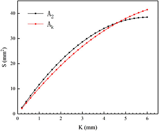
FIGURE 7. The relationship among the cross-sectional area of the orifice and downstream channel and the opening.

To interpret the change of steady-state flow force in the valve, the nephogram of pressure and velocity in the flow channel under different inlet and outlet pressures is shown in Figure 8; at this time, the opening is 1 mm. There is one low-pressure area located near the tip of the valve core, while the other low-pressure area is located at the orifice. When the pressure differential increases gradually, greater pressure variation happens near the orifice. The greater pressure differential is, the larger pressure downstream is. In addition, the size of low pressure area at the orifice gradually increases with the increasing pressure differential. If the low pressure is lower than the saturated vapor pressure of liquid, cavitation will occur (Yuan et al., 2019). Furthermore, the velocity nephogram shows that both the maximum velocity and the average velocity at orifice increase with the increasing pressure differential. The larger pressure differential is, the larger range of high-speed zone is. The high-speed zone is corresponding to the low pressure range. The increment of pressure differential enhances the variation gradient of velocity, and the result is that the variation of pressure gradient near the orifice becomes more obvious. These changes of pressure and velocity in the flow field satisfied Bernoulli equation ignoring the energy loss and gravity potential energy.

FIGURE 8

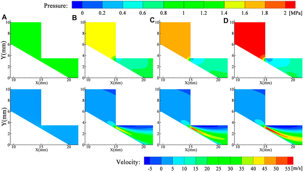
FIGURE 8. Pressure and velocity nephogram with different pressure differentials: (A) Δp = 0.5 MPa; (B) Δp = 0.8 MPa; (C) Δp = 1.1 MPa; (D) Δp = 1. 4 MPa.

To better understand the influence of pressure differential on the flow force, the numerical calculation results of the local pressure distribution along the outline of the valve core tip is shown in Figure 9. The opening and the outlet pressure remain the same, while the inlet pressure increases gradually, that is to say, the pressure differential increases gradually. From Figure 9, we could find that the abscissa of the minimum pressure along the outline of the valve core tip increases gradually with increasing pressure differential, and the position where pressure changes dramatically gradually moved to the valve core tip. The value of this minimum pressure decreases with increasing pressure differential. The changes of the minimum pressure are more obvious under a larger pressure differential.

FIGURE 9

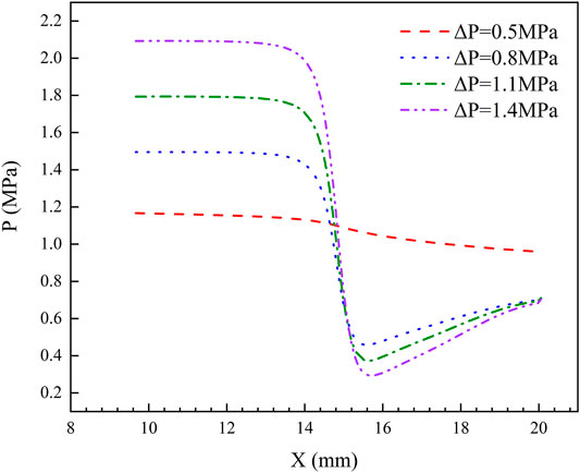
FIGURE 9. The local pressure distribution along the outline of the valve core tip under various differential pressure conditions.

The experimental data, calculation, and simulation results of the axial steady-state flow force under different pressure differentials are shown in Figure 10. The value of axial steady-state flow force increases with the increasing pressure differential at the same opening of the valve. When the differential pressure is 0.3 MPa, the value of flow force is 2.8 N. When the differential pressure increases to 1.4 MPa, the value of flow force reaches 14.1 N. When the pressure difference is small, the flow rate through the orifice is small, which will result in smaller change of fluid momentum, so the steady-state flow force is small. With the gradual increase of the pressure differential, the flow rate and change of fluid momentum through the orifice increase, which also increases the steady-state flow force. The experimental data, calculation, and simulation results agree well with each other, which reveal the reliability and feasibility of the proposed theoretical model. Furthermore, there are also some small deviations among them because of the simplification of the two-dimensional model and assumptions in the calculation. Machining tolerance of the test valve, ignoring the frictional resistance between valve core and valve body, ignoring oil compressibility in the simulation, etc. are all the reasons for this deviation.

FIGURE 10

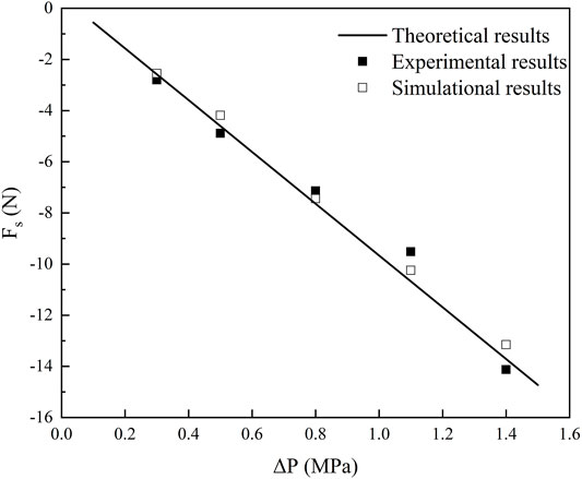
FIGURE 10. The relationship between the differential pressure and steady-state flow force under various differential pressure conditions.

Effects of Opening on Steady-State Flow Force Characteristics of the Valve

Figure 11 shows the pressure and velocity nephogram near the orifice at the same pressure differential and increasing opening of the valve. Although the opening is different, the distribution of pressure is almost the same. The highest pressure is located at the inlet port, and the pressure changes more violently at the orifice. It also could be seen from Figure 11 that there are two low-pressure areas, which locate near the tip of the valve core and the orifice, respectively. With the increase of the valve opening, the pressure decreases first and then increases. The pressure acting on the surface of the valve core will vary with the oil velocity, which satisfies the Bernoulli equation. Furthermore, the change of velocity nephogram shows that the variation of velocity at larger opening is more significant than that at smaller openings. The maximum velocity increases rapidly with increasing valve opening, and the high-velocity area also increases rapidly with increasing valve opening. Also, the average velocity at the orifice rises with increasing opening. Higher flow velocities occurring at the orifice will result in larger value of the flow force.

FIGURE 11

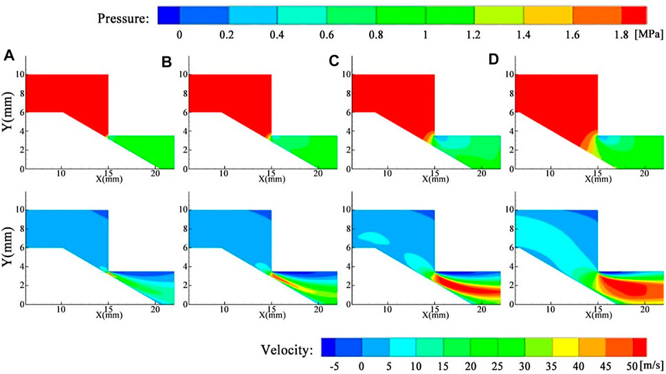
FIGURE 11. Pressure and velocity nephogram at different openings: (A) 0.5 mm; (B) 1 mm; (C) 2 mm; (D) 4 mm.

Figure 12 shows the numerical calculation results of pressure distribution along the outline of the valve core tip at different valve openings. To better demonstrate the change of pressure distribution, this line starts at the bottom of the cone angle. When the opening gradually increases, the pressure along the outline of the valve core tip downstream decreases first and then increases, and the position of the minimum pressure move toward downstream gradually. The position where the dividing point of the pressure near the orifice gradually moves to the cone tip is the same as that shown in the pressure nephogram in Figure 11.

FIGURE 12

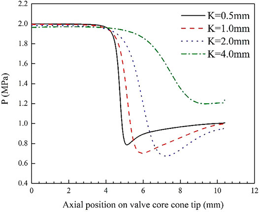
FIGURE 12. Pressure distribution along the outline of the valve core tip at different openings.

Figure 13 shows the variation of the axial steady-state flow force acting on the valve core with changing opening. It could be seen that the value of flow force increases first and then decreases with the increase of opening. When the opening is very small (0–0.5 mm), the flow rate in the valve is relatively small and the momentum change is also small, which will result in small flow force. While the opening of the valve gradually increases (0.5∼2 mm), the flow rate increases significantly, and so does the corresponding change of momentum, which induces a significant increase in the flow force. At the opening of 2 mm, the steady-state fluid force reaches its maximum value. If the opening of the valve is larger than 2 mm, the throttling effect of the conical valve will be seriously affected. Although the flow rate continues to increase, its variation amplitude of momentum begins to decrease, which also decreases the flow force. At the opening of 4–5 mm, the throttling effect of the valve is not obvious; the steady fluid force is tiny but not equal to zero. Furthermore, the change trend of the axial steady-state flow force under different pressure differentials also has similar characteristics.

FIGURE 13

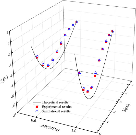
FIGURE 13. The curve of the axial steady-state flow force acting on the valve core with different openings.

The flow force is one of the important factors affecting the performance and control accuracy of the valve, which will lead to poor control performance of the system. Reasonable geometric parameters and operating conditions are beneficial for normal operation of valve, avoiding suffering from the negative impact derived from the flow force, reducing power consumption, and improving efficiency. This paper concerns the rules of how flow force works on the valve core, providing a foundation for the improvement of the valve’s stability.

Conclusion

In this paper, the characteristics of the axial steady-state flow force acting on the internal flow valve core are investigated by theoretical, numerical calculation and experiment investigation. A mathematical model of calculating the steady-state flow force is proposed. Also, the orthogonal test is designed with the help of the four-factor, four-level orthogonal table, which is used to investigate combing geometric parameters and operating conditions affecting the axial steady-state flow force. By extremum difference analysis, the pressure differential and the opening are the main factors affecting the axial steady-state flow force on the internal flow inside the valve. The pressure acting on the surface of the valve core will vary with the changing oil velocity. High flow velocity occurring at the orifice will result in a significant increase in flow force. The larger the pressure differential is, the larger the flow rate and the axial steady-state flow force on the internal flow field of the valve core are. Furthermore, the flow force is small when the opening is very small. With the increase of the valve opening, the flow force increases first and then decreases when the pressure differential remains the same. The results help to improve the reliability, control performance, and service life of the hydraulic systems.

Data Availability Statement

The original contributions presented in the study are included in the article/Supplementary Material, further inquiries can be directed to the corresponding author.

Author Contributions

XL and JH contributed to the conception and design of the study. JM, YZ, SX, and QL contributed to comprehensive tests. BL and FX contributed to discussion. All authors contributed to article revision and read and approved the submitted version.

Funding

This work was supported by the National Natural Science Foundation of China (Grant Number 51875559), the Fundamental Research Funds for the Central Universities (Grant Number 2015XKMS026), and the Priority Academic Program Development of Jiangsu Higher Education Institutions (PAPD).

Conflict of Interest

The authors declare that the research was conducted in the absence of any commercial or financial relationships that could be construed as a potential conflict of interest.

Publisher’s Note

All claims expressed in this article are solely those of the authors and do not necessarily represent those of their affiliated organizations, or those of the publisher, the editors, and the reviewers. Any product that may be evaluated in this article, or claim that may be made by its manufacturer, is not guaranteed or endorsed by the publisher.

References

Filo, G., Lisowski, E., and Rajda, J. (2019). Flow Analysis of a Switching Valve with Innovative Poppet Head Geometry by Means of CFD Method. Flow Meas. Instrumentation 70, 101643. doi:10.1016/j.flowmeasinst.2019.101643

CrossRef Full Text | Google Scholar

Gao, L., Wu, C., Zhang, D., Fu, X., and Li, B. (2019). Research on a High-Accuracy and High-Pressure Pneumatic Servo Valve with Aerostatic Bearing for Precision Control Systems. Precision Eng. 60, 355–367. doi:10.1016/j.precisioneng.2019.09.005

CrossRef Full Text | Google Scholar

Han, M., Liu, Y., Wu, D., Zhao, X., and Tan, H. (2017). A Numerical Investigation in Characteristics of Flow Force under Cavitation State inside the Water Hydraulic Poppet Valves. Int. J. Heat Mass Transfer 111, 1–16. doi:10.1016/j.ijheatmasstransfer.2017.03.100

CrossRef Full Text | Google Scholar

Jia, W., Yin, C., Hao, F., Li, G., and Fan, X. (2019). Dynamic Characteristics and Stability Analysis of Conical Relief Valve. mech 25 (1), 25–31. doi:10.5755/j01.mech.25.1.22881

CrossRef Full Text | Google Scholar

Kang, J., Yuan, Z., and Tariq Sadiq, M. (2020). Numerical Simulation and Experimental Research on Flow Force and Pressure Stability in a Nozzle-Flapper Servo Valve. Processes 8 (11), 1404. doi:10.3390/pr8111404

CrossRef Full Text | Google Scholar

Lain, S., Broder, D., Sommerfeld, M., and Goz, M. F. (2002). Modelling Hydrodynamics and Turbulence in a Bubble Column Using the Euler-Lagrange Procedure. Int. J. Multiphase Flow 28 (8), 1381–1407. doi:10.1016/s0301-9322(02)00028-9

CrossRef Full Text | Google Scholar

Lei, J., Tao, J., Liu, C., and Wu, Y. (2018). Flow Model and Dynamic Characteristics of a Direct spring Loaded Poppet Relief Valve. Proc. Inst. Mech. Eng. C: J. Mech. Eng. Sci. 232 (9), 1657–1664. doi:10.1177/0954406217707546

CrossRef Full Text | Google Scholar

Li, L., Yan, H., Zhang, H., and Li, J. (2018). Numerical Simulation and Experimental Research of the Flow Force and Forced Vibration in the Nozzle-Flapper Valve. Mech. Syst. Signal Process. 99, 550–566. doi:10.1016/j.ymssp.2017.06.024

CrossRef Full Text | Google Scholar

Liang, J., Luo, X., Liu, Y., Li, X., and Shi, T. (2016). A Numerical Investigation in Effects of Inlet Pressure Fluctuations on the Flow and Cavitation Characteristics inside Water Hydraulic Poppet Valves. Int. J. Heat Mass Transfer 103, 684–700. doi:10.1016/j.ijheatmasstransfer.2016.07.112

CrossRef Full Text | Google Scholar

Lin, T., Chen, Q., Ren, H., Lv, R., Miao, C., and Chen, Q. (2018). Computational Fluid Dynamics and Experimental Analysis of the Influence of the Energy Recovery Unit on the Proportional Relief Valve. Proc. Inst. Mech. Eng. Part C: J. Mech. Eng. Sci. 232 (4), 697–705. doi:10.1177/0954406216687790

CrossRef Full Text | Google Scholar

Park, S., and Rhee, S. H. (2012). Computational Analysis of Turbulent Super-cavitating Flow Around a Two-Dimensional Wedge-Shaped Cavitator Geometry. Comput. Fluids 70, 73–85. doi:10.1016/j.compfluid.2012.09.012

CrossRef Full Text | Google Scholar

Scuro, N. L., Angelo, E., Angelo, G., and Andrade, D. A. (2018). A CFD Analysis of the Flow Dynamics of a Directly-Operated Safety Relief Valve. Nucl. Eng. Des. 328, 321–332. doi:10.1016/j.nucengdes.2018.01.024

CrossRef Full Text | Google Scholar

Tan, L., Xie, H., Chen, H., and Yang, H. (2019). Structure Optimization of Conical Spool and Flow Force Compensation in a Diverged Flow Cartridge Proportional Valve. Flow Meas. Instrumentation 66, 170–181. doi:10.1016/j.flowmeasinst.2019.03.006

CrossRef Full Text | Google Scholar

Xie, H., Tan, L., Liu, J., Chen, H., and Yang, H. (2018). Numerical and Experimental Investigation on Opening Direction Steady Axial Flow Force Compensation of Converged Flow Cartridge Proportional Valve. Flow Meas. Instrumentation 62, 123–134. doi:10.1016/j.flowmeasinst.2018.05.013

CrossRef Full Text | Google Scholar

Yang, H., Wang, W., and Lu, K. (2019). Cavitation and Flow Forces in the Flapper-Nozzle Stage of a Hydraulic Servo-Valve Manipulated by Continuous Minijets. Adv. Mech. Eng. 11 (5), 168781401985143. doi:10.1177/1687814019851436

CrossRef Full Text | Google Scholar

Yang, H., Wang, W., and Lu, K. (2019). Numerical Simulations on Flow Characteristics of a Nozzle-Flapper Servo Valve with Diamond Nozzles. Ieee Access 7, 28001–28010. doi:10.1109/access.2019.2896702

CrossRef Full Text | Google Scholar

Ye, Y., Yin, C.-B., Li, X.-D., Zhou, W.-j., and Yuan, F.-f. (2014). Effects of Groove Shape of Notch on the Flow Characteristics of Spool Valve. Energ. Convers. Manag. 86, 1091–1101. doi:10.1016/j.enconman.2014.06.081

CrossRef Full Text | Google Scholar

Yuan, C., Song, J., Zhu, L., and Liu, M. (2019). Numerical Investigation on Cavitating Jet inside a Poppet Valve with Special Emphasis on Cavitation-Vortex Interaction. Int. J. Heat Mass Transfer 141, 1009–1024. doi:10.1016/j.ijheatmasstransfer.2019.06.105

CrossRef Full Text | Google Scholar

Zhang, Z., Jia, L., and Yang, L. (2019). Numerical Simulation Study on the Opening Process of the Atmospheric Relief Valve. Nucl. Eng. Des. 351, 106–115. doi:10.1016/j.nucengdes.2019.05.034

CrossRef Full Text | Google Scholar

Zong, C., Zheng, F., Chen, D., Dempster, W., and Song, X. (2020). Computational Fluid Dynamics Analysis of the Flow Force Exerted on the Disk of a Direct-Operated Pressure Safety Valve in Energy System. J. Press. Vessel Technol-trans ASME 142 (1), 14. doi:10.1115/1.4045131

CrossRef Full Text | Google Scholar