Research on Unsteady Wake Characteristics of the NREL 5MW Wind Turbine Under Yaw Conditions Based on a LBM-LES Method

The yaw of a large-scale wind turbine will change the aerodynamic performance of its substructures. In view of this, this article applied a LBM-LES method to numerically simulate the yawed MEXICO wind turbine and compared the numerical results with the experimental data collected in the New MEXICO experiment to verify the reliability of the method. A rapid dynamic yaw is defined with a yaw speed of 5°/s in yaw control, while a slow dynamic yaw is with a yaw speed of 0.3°/s. The NREL 5 MW offshore wind turbine was used to explore the constant wake characteristics under the conditions of a rapid dynamic yaw and of a slow dynamic yaw. It can be seen from the results that the LBM-LES method captures the detailed characteristics of the complex unsteady flow field of the wind turbine. In the rapid dynamic yaw process, the transition area between the far wake and the near wake shows a large deflection. However, in the process of the slow dynamic yaw, the far wake deflects forward relatively to the yaw. The dynamic yaw wake forms a kidney-shaped cross-section similar to the one in a steady yaw. The yaw wake recovers faster than the wake without yaw, and the rapid dynamic yaw wake has an asymmetric structure. The thrust of the wind turbine drops rapidly during the rapid dynamic yaw, while the thrust of the slow dynamic yaw decreases gradually. The thrust drops three times per rotor revolution, and the time of thrust decrease is delayed as the yaw angle increases.

Introduction

Wind power is one of the important clean energy sources today, which can effectively alleviate the global warming and promote a low-carbon economy (Dai et al., 2018). With the continuous progress of wind power technology, the installed capacity of wind power continues to increase (Kress et al., 2015). The turbulence, wind speed, wind direction, yaw, and terrain of the atmospheric boundary layer have their respective impacts on the unsteady wake characteristics of wind turbines (Han et al., 2018). Extreme wind conditions, such as wind gusts or sudden changes in wind direction, may result in changes in fatigue load and aerodynamic field. Under these extreme conditions, the operation of wind turbines generates complex three-dimensional unsteady flow characteristics that can have a considerable impact on downwind turbines. Due to the complexity of the rotating rotor, a full-scale aerodynamic simulation is undoubtedly challenging and consumes a lot of computing resources. Therefore, an effective method to simulate the wake characteristics of wind turbines is required.

The lattice Boltzmann method (LBM) is a popular method to simulate flows and hydrodynamic interactions in incompressible fluids (Kaoui, 2020); the particles of the fluid exist on discrete grid nodes and migrate along the grid chain. In addition, all the particles collide and migrate synchronously with each other following certain collision rules. In recent years, LBM is also applicable to the research in wind energy. Many attempts have been made in the past (Kim et al., 2012; Di Ilio et al., 2018; Khan, 2018) to study wind turbines using the LBM method. Good consistent results of the flow field and wake characteristics were obtained. Xu (2016) simulated a single turbine and three in-line turbines with the LBM model to capture the wake evolutions, and explored the detailed flow characteristics. Deiterding and Wood (2016a); Deiterding and Wood (2016b) studied three Vestas V27 wind turbines by the LBM at a prescribed rotation rate and under constant inflow conditions, and explored that the model can predict the vortex structure downstream at a moderate computational cost. Rullaud et al. (2018) combined the LBM and the actuator line method to simulate the vertical axis wind turbine, and analyzed the force and wake velocity. In addition, the adaptive mesh refinement (AMR) method allows the lattice cells to be automatically refined to allocate more grid points on the wind turbine walls and wake area. Wood and Deiterding (2015) established a novel parallel adaptive LBM, which predicted the power and thrust coefficients of Vestas V27 turbines with a high accuracy, including the tower and ground interaction. With the help of AMR, Li et al. (2020) utilized the LBM-LES method to simulate the wake trajectory of the MEXICO wind turbine, and analyzed the characteristics of transient wake propagation, rotor-tower interaction, wake, and the effect of tip-speed ratio. In short, it was found that LBM can easily handle the complex geometry of wind turbines, so LBM is suitable for simulating the interaction between wind turbines and airflow.

The aerodynamics of wind turbines under yaw has been studied by experiments and numerical simulations. In the MEXICO experiment, Snel et al. (2007); Pereira et al. (2013) measured the aerodynamic parameters of wind turbines under different working cases such as axial flow and yaw, and used particle image velocimetry (PIV) to measure the flow field. Macrí et al. (2021) used the stereo particle imaging velocimetry method to study the far wake response of a yawing upstream wind turbine, and the results showed the influence of the yaw maneuvering direction on its time dynamics. Many accurate numerical models under yaw were given in the references, such as the three-dimensional yawed wake model proposed by Cortina et al. (2017) for the estimation of the noncentrosymmetric cross-sectional shape of the yawed wake velocity distribution. Based on the conservation of momentum and the top-hat model that Jensen (1983) predicted the wake deflection effect, Jiménez et al. (2010) applied the LES model under particular wind boundary conditions to simulate and characterize the wake deflection based on a range of yaw angles of the turbine. Bastankhah and Porté-Agel (2015) proposed an analytical model based on the experimental analysis to predict the wake deflection and wake distribution in the far wake for a steady yaw.

Dynamic yaw is a continuous rotation process with a constant or variable rotation speed, and it was found that the unsteady aerodynamic characteristics of a wind turbine under a 3D dynamic yaw still need to be studied (Ye et al., 2020). Qiu et al. (2014) proposed a free vortex method to study the blade torque and wake of the NREL phase VI wind turbine under a rapid dynamic yaw process with a constant yaw rate of 5°/s and 20°/s. Leble and Barakos (2017) applied numerical simulations to study the slow dynamic yaw performance of the DTU 10-MW wind turbine with a yaw rate of 0.3°/s and a yaw amplitude of 3°/s. The results showed that the total power under the slow dynamic yaw conditions was much greater than the static yaw conditions. Wen et al. (2019) applied the free vortex method to study the sinuous motion of the NREL 5-MW with an average yaw rate of 1.2°/s and 2.4°/s. The results showed that the dynamic yaw motion caused the upwind and downwind yaw effects, which have a greater impact on the angle of attack of the blade sections. Then, Wang et al. (2019) applied the Unsteady Reynolds-averaged Navier-Stokes to study the slow dynamic yaw on the start and stop process of wind turbines with yaw rates of 0°/s–0.3°/s, and the results showed that the increase of yaw rate led to larger load fluctuations during the process of start and stop of wind turbine.

All in all, the dynamic yaw process of wind turbines will affect the aerodynamic performance of the impeller and wake structure, but the current research on the issue is still insufficient. The current research on the dynamic yaw mainly focuses on the steady-state yaw angle and the process of slow dynamic yaw. However, in actual operation, the dynamic yaw of a wind turbine exhibits a process of slow and continuous change, and a rapid dynamic yaw will occur under extreme wind shear conditions (Jing et al., 2020). When the wind direction changes rapidly under extreme wind conditions, the controller waits to command the yaw control and the rotor does not directly face the inflow wind direction. Therefore, it is necessary to study the complex wake and aerodynamic characteristics in the rapid dynamic yaw process and slow dynamic yaw process. The present work aims to apply the LBM-LES method to calculate the dynamic yaw of wind turbines. The main contribution of this article is to investigate the yaw wake characteristics of wind turbines under the LBM-LES method. First, we applied the New MEXICO experimental results to validate the LBM-LES method about its prediction of the yaw wake information, then we investigated the dynamic yaw characteristics of the wind turbine with the method. The other objective of this study is to study the unsteady characteristics of the slow dynamic yaw and rapid dynamic yaw of a large wind turbine. In this purpose, we analyzed the three-dimensional unsteady characteristics of the NREL 5 MW offshore wind turbine under the conditions of a rapid dynamic yaw (5°/s) and a slow dynamic yaw (0.3°/s).

Theoretical Analysis

Numerical Models

Lattice Boltzmann Method

The lattice Boltzmann method (LBM) is a discretization of the Boltzmann-BGK equations in terms of space, time, and velocity. The velocity of a particle is simplified into a finite-dimensional velocity space $\left\{e_0,e_1,\cdots ,e_{\alpha },\cdots ,e_N\right\}$ where N denotes the kind of velocity, and the continuous distribution function f is discretized accordingly as $\left\{f_0,f_1,\cdots ,f_{\alpha },\cdots ,f_N\right\}$, and the discrete velocity equation is expressed as follows (Kim et al., 2012):

$\begin{array}{cc}\frac{\partial f_{\alpha }}{\partial t}+e_{\alpha }\cdot \nabla f_{\alpha }=-\frac{1}{{\tau }_0}\left(f_{\alpha }-f_{\alpha }^{eq}\right)+F_{\alpha }& \alpha =\mathrm{1,2,}\mathrm{...}\mathrm{,}N\end{array}(1)$

where $f_{\alpha }=f_{\alpha }(r,e_{\alpha },t)$ refers to the number of molecules of velocity at point r and time t, e_α represents the corresponding discrete velocity, and F_α stands for the external force in the discrete velocity space. The discrete-time and space, evolution equation of the lattice Boltzmann-BGK (LBGK) model, is obtained as:

$f_{\alpha }(r+e_{\alpha }{\delta }_t,t+{\delta }_t)-f_{\alpha }(r,t)=-\frac{1}{\tau }\left[f_{\alpha }(r,t)-f_{\alpha }^{eq}(r,t)\right]+{\delta }_t{F}_{\alpha }(r,t)(2)$

where ${\delta }_t$ refers to the time step and $\tau ={\tau }_0/{\delta }_t$ represents the dimensionless relaxation time.

The symmetry of the discrete velocity determines whether the corresponding LBM model can be restored to the required macro equation. The DmQn series model proposed by QIAN et al. (1992) is the basic model of LBM. m refers to the problem dimension and n denotes the number of lattice chains in the velocity model. The DmQn series model adopts the form of the equilibrium distribution function, expressed as follows:

$f_{\alpha }^{eq}\left(r,t\right)=\rho {\omega }_{\alpha }\left[1+\frac{e_{\alpha }\cdot u}{c_s^2}+\frac{{\left(e_{\alpha }\cdot u\right)}^2}{2c_s^4}-\frac{u^2}{2c_s^2}\right](3)$

where ρ refers to the fluid density, u represents the macroscopic velocity, c_s denotes the lattice sound velocity, and ω_α is the density weighting factors:

${\omega }_{\alpha }=\{\begin{array}{c}8/27,\alpha =0\\ 2/27,\alpha =\mathrm{1,2},\mathrm{...},6\\ 1/54,\alpha =\mathrm{7,8},\mathrm{...},18\\ 1/216,\alpha =\mathrm{19,20},\mathrm{...},26\end{array}(4)$

In this article, the D3Q27 model is applied to solve the three-dimensional problem. There are 27 velocity vectors in the D3Q27 model (Cheng et al., 2012), and all directions are considered. The 27 velocity vectors correspond to the distribution functions $f_0$ to $f_{26}$. At this time, the distribution function is $f={\left(f_0,f_1,f_2,\dots ,f_{26}\right)}^T$, and the discrete velocity is as follows:

$e_{\alpha }=\{\begin{array}{c}\left(\mathrm{0,0,0}\right),\alpha =0\\ c\left(\pm \mathrm{1,0,0}\right),c\left(0,\pm \mathrm{1,0}\right),c\left(\mathrm{0,0},\pm 1\right),\alpha =\mathrm{1,2},\mathrm{...},6\\ \mathit{ }c\left(\pm 1,\pm \mathrm{1,0}\right),c\left(\pm \mathrm{1,0},\pm 1\right),c\left(0,\pm 1,\pm 1\right),\alpha =\mathrm{7,8},\mathrm{...},18\mathrm{ }\\ c\left(\pm 1,\pm 1,\pm 1\right),\alpha =\mathrm{19,20},\mathrm{...},26\mathrm{ }\end{array}(5)$

where $c={\delta }_x/{\delta }_t$, ${\delta }_x$, and ${\delta }_t$ refer to the lattice step and time step, respectively, and the lattice steps in the x and y directions are usually the same. c represents the lattice migration rate, which is related to the lattice sound velocity c_s:

$c_s=\frac{\sqrt{3}}{3}c(6)$

In different directions, the LBM equation is:

$f_{\alpha }(r+e_{\alpha }{\delta }_t,t+{\delta }_t)-f_{\alpha }(r,t)={\Omega }_{\alpha },\alpha =\mathrm{0,1},\cdots ,26(7)$

where ${\Omega }_{\alpha }$ can be written as:

${\Omega }_{\alpha }=-M^{-1}S\left[m_{\alpha }(r,t)-m_{\alpha }^{eq}(r,t)\right],\alpha =\mathrm{0,1},\cdots ,26(8)$

where $m_{\alpha }(r,t)$ and $m_{\alpha }^{eq}(r,t)$ refer to the moment and equilibrium function, respectively. S represents the collision matrix, and M stands for a 27 × 27 matrix which linearly transforms the distribution function to the moment:

$m_{\alpha }\left(r,t\right)=M·f_{\alpha }(r,t)(9)$

Governing Equation

In traditional mesh-based CFD approaches, the Navier–Stoles (N–S) equations can be derived from the continuum assumption. Similarly, the weakly compressible N–S equation (Yuan et al., 2017) can be obtained by applying a Chapman–Enskog expansion procedure (Chapman and Cowling, 1970) to Boltzmann Eq. 7.

$\frac{\partial \rho }{\partial t}+\nabla ·\left(\rho u\right)=0(10)$

$\frac{\partial u}{\partial t}+(u\nabla )·u=-\frac{\nabla p}{\rho }+\nu {\nabla }^{2}u(11)$

The Chapman–Enskog extension process is introduced in the reference (Hähnel, 2004). The above N–S equations describe the flow of incompressible fluids, where u refers to the flow velocity, ν represents the kinematic viscosity, and p is the pressure.

Large Eddy Simulation

In the LBM, the LES method is usually used and it is assumed that partial density distribution functions used in the scheme represent the analytical scale. In order to consider the influence of sub-grid scale turbulence, a turbulent viscosity is added to the physical viscosity (Wood and Deiterding, 2015).

$\nu ={\nu }_0+{\nu }_t(13)$

where ν₀ represents the fluid molecular viscosity and ν_t is the turbulent viscosity.

The fluid molecular viscosity coefficient ν₀ is given as (Dong and Sagaut, 2008):

${\nu }_0=\frac{UL}{\mathrm{Re}}(14)$

where U is the velocity reference scale and L is the reference length scale.

We applied the WALE model as the subgrid turbulence model (viz., the turbulent viscosity coefficient ν_t). The WALE model is suitable for LES in complex terrain areas (Wu et al., 2020). In the WALE model, the SGS eddy-viscosity is expressed as follows (Nicoud and Ducros, 1999):

$v_{SGS}={\left(C_W\mathrm{\Delta }\right)}^2\frac{{\left({\overline{S}}_{ij}^d{\overline{S}}_{ij}^d\right)}^{3/2}}{{\left({\overline{S}}_{ij}{\overline{S}}_{ij}\right)}^{5/2}+{\left({\overline{S}}_{ij}^d{\overline{S}}_{ij}^d\right)}^{5/4}}(15)$

where C_W refers to the WALE model constant, 0.2 (Vashahi and Lee, 2018), Δ denotes the filter width, and ${\overline{S}}_{ij}$ is the filtered strain rate tensor, expressed as (Li et al., 2018):

${\overline{S}}_{ij}=\frac{1}{2}\left(\frac{\partial {\overline{u}}_i}{\partial x_j}+\frac{\partial {\overline{u}}_j}{\partial x_i}\right)(16)$

and ${\overline{S}}_{ij}^d$ represent the traceless symmetric part of the square of the velocity gradient tensor expressed as:

${\overline{S}}_{ij}^d=\frac{1}{2}\left({\left(\frac{\partial \overline{u_i}}{\partial x_j}\right)}^2+{\left(\frac{\partial \overline{u_j}}{\partial x_i}\right)}^2\right)-\frac{1}{3}{\delta }_{ij}{\left(\frac{\partial \overline{u_k}}{\partial x_k}\right)}^2(17)$

Simulation Setup

Reference Wind Turbines

As shown in Figure 1, the MEXICO wind turbine used in this study is a three-blade machine with a blade length of 2.25 m and a tower height of 5.12 m, and the root, middle, and tip regions of the blade are selected from three types of airfoils of the DU, Risø, and NACA airfoil series, respectively. The MEXICO and New MEXICO experiments were conducted in the German–Netherlands DNW wind tunnel. In the MEXICO experiment, in 2006 (Pereira et al., 2013), a large amount of experimental data were recorded under various operating cases (Snel et al., 2007). Furthermore, the New MEXICO experiment was performed to improve the database in 2014. The New MEXICO experiment was calibrated and tested for different roughness applications in the blade outboard area, and the flow field of the axial flow and yaw cases were tested with a particle image velocimetry (PIV) (Boorsma and Schepers, 2014). The current work uses the results from both MEXICO and New MEXICO experiments, and uses data under similar yaw conditions for verification. As shown in Figure 2, the New MEXICO yaw (a yaw angle of ϒ = 30°) measurement tested the flow field results in the horizontal plane of the hub height, which was the axial traverse of velocity in the plane of $z=-1\text{.}5\text{ m}$, $z=1\text{.}5\text{ m}$, and the radial traverse of velocity parallel to the wind turbine plane includes $x^{\prime }=-0.3\text{m}$ (upwind) and $x^{\prime }=0.3\text{m}$ (downwind). The average values of the axial, radial, and tangential components of the velocity were calculated by the circumferential average method. In this study, the case corresponding to a wind speed of (U = 15 m/s; tip-speed ratio: λ= 6.67) is considered, which represents the turbulent wake state, design condition, and separated flow condition. The operating condition in the present simulations is a yaw angle of 30°, a pitch angle of 2.3°, and a rotation speed of 424.5 rpm.

FIGURE 1

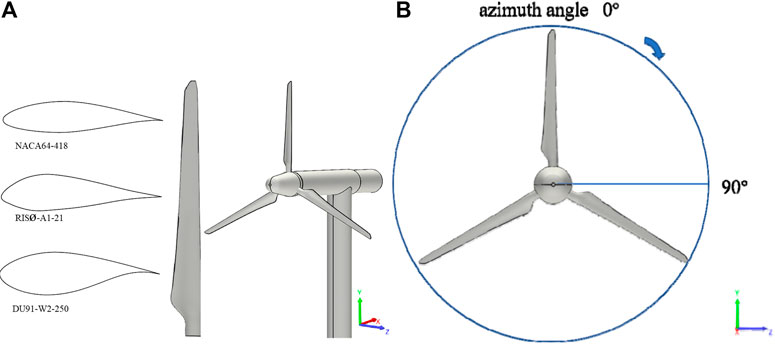
FIGURE 1. Geometry of the MEXICO wind turbine: (A) blade airfoil and turbine model; (B) diagram of the blade azimuth angle.

FIGURE 2

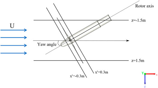
FIGURE 2. Location of measurement data in the New MEXICO experiment.

Numerical Set-Up

In the New MEXICO experiment, the turbine was placed in an open 9.5 m × 9.5 m configuration, and the turbine was placed 7 m downstream of the inlet, the length of the measuring part was 20 m, the turbulence intensity was estimated to be below 0.4%. For all our simulations, the computational domain is shown in Figure 3, the length, width, and height of the computational domain are set to 12D × 4D × 4D, which was chosen according to the reference Li et al. (2020). The wind turbine placed 2D downstream of the inlet boundary in simulation, and D refers to the diameter of the turbine, 4.5 m. Remark that in the experiment the rotor was placed at less than 2D downstream of the inlet. The inlet is set as a velocity inlet with a turbulence intensity of 0.4%, and the outlet is a free outlet. The bottom surface is set to be the ground wall, the remaining surfaces are set symmetrically, and the boundaries of the turbine are set as no-slip walls.

FIGURE 3

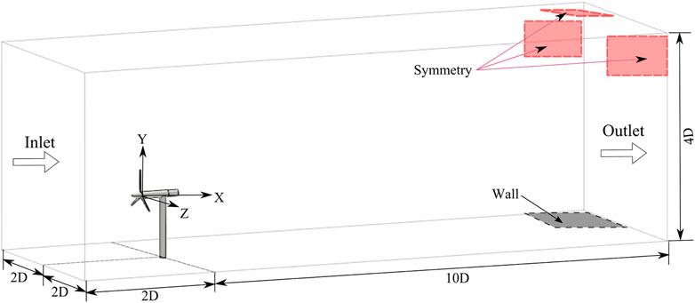
FIGURE 3. Physical domain used in the study.

The fluid domain is automatically divided into lattices through LBM, and the accuracy of physical boundaries and flow characteristics depends on the division size of the lattices. Moreover, adding the lattices of the wind turbine can improve the calculation accuracy of the flow field. The AMR method (Wood and Deiterding, 2015) is an effective method that only dynamically allocates fine grids to key positions. Chen et al. (2014) introduced a detailed boundary processing method, and assigned the rebound boundary conditions of the wind turbine, which is a direct method for both static and moving boundaries. Therefore, the boundary nodes are generally fluid nodes next to the physical nodes, and the physical boundary is located in the middle. Since the articles pays special attention to the wake characteristics, the AMR method is applied to improve the simulation accuracy of the blade and wake characteristics. The adaptation of wind turbine blades and surrounding wakes is achieved through an octree structure lattice to achieve a nonuniform structure. Therefore, there are different spatial scales at different locations in the fluid domain. The grid width is selected as the filter length in the LES calculation, and the grid is dynamically refined in the wake region characterized by the magnitude of the vorticity. To ensure constant Courant–Friedrichs–Lewy (CFL) conditions and sound velocity at any location in the domain, the ratio of space to time is maintained throughout the domain. Meanwhile, different levels of grids communicate through the interpolation scheme introduced by Yuan et al. (2017).

To explore the influence of both rapid and slow dynamic yaw on the unsteady wake characteristics of large wind turbines, the NREL 5 MW offshore reference wind turbine is utilized, which was designed by the National Renewable Energy Laboratory (NREL) (Nejad et al., 2016). The rotor diameter is 126 m, the tower height is 90 m, and the rated rotational speed is 12.1 rpm with the rated wind speed U = 11.4 m/s. Figure 4 shows the change of the yaw angle with time in the simulation of a slow and a rapid dynamic yaw. The rapid dynamic yaw is based on the extreme wind shear setting of IEG-61400-1 (Jing et al., 2020), which covers a 30° yaw angle within 6 s. Meanwhile, the unsteady calculation is performed within the first 200 s, and the rapid dynamic yaw starts when the calculation is stabilized, and the dynamic process lasts for 6 s. For the slow dynamic yaw, the yaw speed is set to 0.3°/s for the yaw control and the unsteady calculation without yaw before t = 150 s. Starting from t = 150 s, the wind turbine yaws at a speed of 0.3°/s until t = 300 s, and the yaw process is completed with a yaw angle of ϒ = 45°.

FIGURE 4

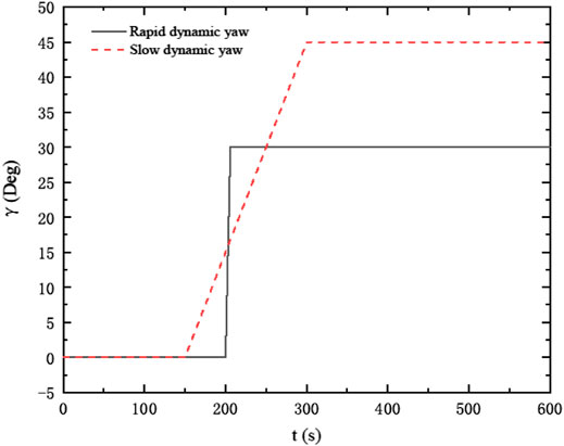
FIGURE 4. Diagram of the yaw angle with time in the slow and rapid dynamic yaw.

The calculation time step for the MEXICO wind turbine is set to 0.0039206 s, that is, for each time step, the wind turbine rotates 10° with an overall physical time of 20 s. The maximum lattice solution scale of the computational domain is 2 m, the lattice solution scale of the nacelle and the tower is 0.03125 m. Xu (2016) gave a finest resolution scale of 0.1 m for the NREL phase VI wind turbine, and Deiterding and Wood (2016a) gave a finest resolution scale of 0.015625 m for the MEXICO turbine, thus, we set the solution scale of the New MEXICO wind turbine to 0.015625 m, and the solution scale of the wake region is set to 0.03125 m. However, the calculation time step of the NREL 5 MW wind turbine is set to 0.125 s with an overall physical time of 600 s. The maximum lattice solution scale of the computational domain is 28 m, the lattice solution scale of the nacelle and tower is 0.875 m, the solution scale of the rotor is set to 0.4375 m, and the solution scale of the wake area is set to 0.875 m. The simulations were done on an HP workstation with two E5 CPUs including 32 cores, and each simulation took about 14 days. The screenshot of adaptive mesh elements of the NREL 5 MW turbine at t = 40 s is shown in Figure 5. Traditional LES simulation needs to set fine grids on the blade surface. However, in LBM, the rotor is encrypted, and the wake is optimized through dynamic adaptive tracking, which allows an automatic refinement and an allocation of more grids in the wake area. The minimum lattice size will limit the increase in huge calculations. The purpose of this article is to use the LBM to achieve an accurate simulation of wind turbine wake with a small grid cost. Future research work should investigate the accuracy of blade grids.

FIGURE 5

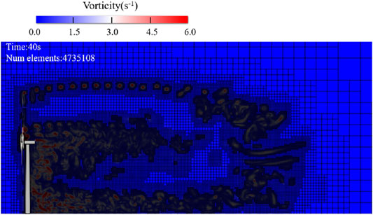
FIGURE 5. Screenshot of the adaptive mesh elements of the NREL 5 MW turbine at t = 40 s during a calculation.

Results and Discussion

Verification of the New Model Rotor Experiments in Controlled Conditions

Figure 6 shows the comparison of axial traverse of velocity in two different directions at $z=1\text{.}5\text{ m}$ and $z=-1\text{.}5\text{ m}$. In this figure, u/v/w represents the traverse of velocity in x-direction, y-direction, and z-direction of the physical domain (Figure 4). On the right side (+z axis) of the wind turbine, $z=1\text{.}5\text{ m}$ is far from the nacelle along the axial direction, and the influence of the nacelle disappears. The calculated velocity component u decreases behind the wind turbine, and the calculated values are slightly lower than the experimental values. With the increase of the distance from the wind wheel, the degree of wake deflection increases, and the degree of wake deflection in the numerical simulation is higher than in the experiment. The velocity component v increases first and then decreases along the x-axis, and the calculated value at the center of the wind turbine (x = 0) is higher than the experimental value by 1 m/s. The change of the axial velocity and radial velocity is slight, but that of the tangential velocity is great. The LBM fails to capture the significant velocity change behind the rotor plane. It may be that the bound vortex on the blade is relatively small, and the mesh resolution is not increased during the adaptive refinement of mesh in the wake area, resulting in faster dissipation of the shed vortices. However, the model accurately predicted the blade root vortex and the blade tip vortex. As the wake away from the rotor plane develops, the degree of wake deflection calculated using the numerical simulation increases constantly, which is greater than the experimental result. The structure of the tip vortex fails to be captured by the velocity components along the axis, as it is far away from the axes at $z=1\text{.}5\text{ m}$. The velocity component w fluctuates more strongly than u and v behind the wind wheel, and the speed fluctuation caused by the tip vortex is not captured behind the wind turbine.

FIGURE 6

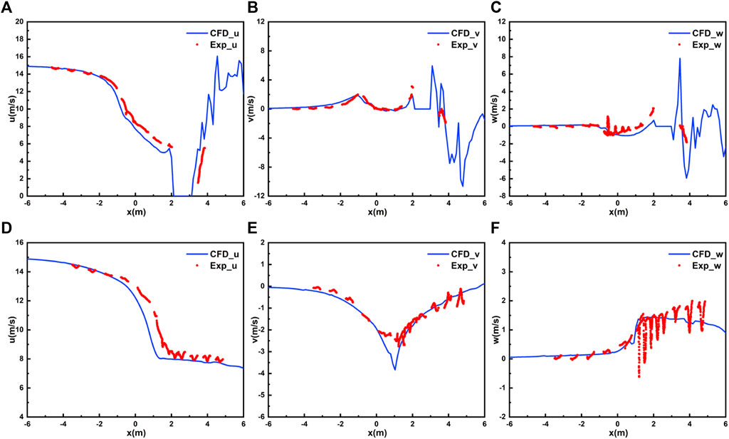
FIGURE 6. Comparison of simulation values and experiment results of axial traverse of velocity in different direction in the horizontal plane of the hub height: (A) axial velocity at $z=-1\text{.}5\text{ m}$, u; (B) radial velocity at $z=-1\text{.}5\text{m}$, v; (C) tangential velocity at $z=-1\text{.}5\text{m}$,w; (D) axial velocity at $z=1\text{.}5\text{ m}$, u; (E) radial velocity at $z=1\text{.}5\text{m}$, v; (F) tangential velocity at $z=1\text{.}5\text{ m}$, w.

Figure 7 shows the comparison of radial traverse of velocity in two different directions at $x^{\prime }=-0.3\text{m}$ (as shown in Figure 4, upwind) and $x^{\prime }=0.3\text{m}$ (downwind) of the wind turbine, respectively. In addition, the calculating time t = 20 s, and the azimuth angle is 0°. In the upwind ($x^{\prime }=-0.3\text{m}$), the velocity component u decreases from 15 m/s to 11 m/s because of the wind turbine blockage effect. Due to the existence of the hub, the velocity component (u, v, w) is zero within the range of 0.2 m < r < 0.2 m. Moreover, all velocity components are consistent with the experimental values. When the airflow passes through the wind turbine, the speed is significantly reduced, particularly the velocity component u on the radial blade tip $x^{\prime }=-0.3\text{m}$, which is decreased to 8 m/s. The axial velocity u increases slowly from the blade tip to root, and a large axial velocity appears at the blade root, distributing on both sides of the nacelle due to the inductive effect of the blade root vortex. In the downwind, the calculated u/v/w distributing along with the radial direction is consistent with the experimental data, and the velocity component increment caused by the blade tip vortex and the blade root vortex at the blade tip and root is captured by the model.

FIGURE 7

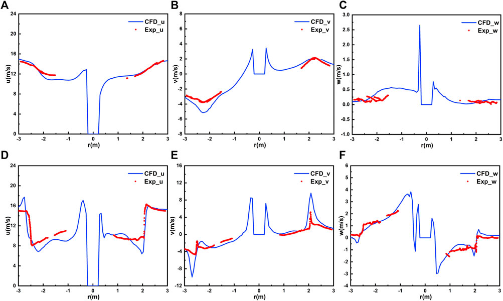
FIGURE 7. Comparison of simulation values and experiment results of radial traverse of velocity in different directions in the horizontal plane of the hub height: (A) axial velocity at $x^{\prime }=-0.3\text{m}$, u; (B) radial velocity at $x^{\prime }=-0.3\text{m}$, v; (C) tangential velocity at $x^{\prime }=-0.3\text{m}$, w; (D) axial velocity at $x^{\prime }=0.3\text{m}$, u; (E) radial velocity at $x^{\text{'}}=0.3\text{m}$,v; (F) tangential velocity at $x^{\text{'}}=0.3\text{m}$,w.

Figure 8 shows the instantaneous wake structure (Figure 8A) and velocity contour of the different vertical sections under ϒ = 0° (Figure 8A) and ϒ = 30° (Figure 8C), respectively. The wake structure could be observed in a three-dimensional instantaneous iso-surface, in which the tip vortex falls off the tip and develops in a spiral shape. The upwind blade tip vortex interacts with the shedding vortex caused by the hub, and breaks into a small-scale vortex during its downward development. The wake of the wind turbine gradually recovers with the increase of the distance from the wind turbine. The wake at ϒ = 0° is symmetrically distributed along the centerline of the wind turbine, however, the wake at ϒ = 30° is asymmetrically distributed in the horizontal and vertical directions, which is expected and is in agreement with previous studies by Jiménez’s theoretical analysis (Jiménez et al., 2010; Abkar and Porté-Agel, 2015): the asymmetric distribution of the wake deflection angle relative to the wake center. As shown in the far-wake area of Figure 8C, the wake forms a kidney-shaped cross-section. Howland et al. (2016) analyzed the development of far wake to obtain a higher deflection which forms a counter-rotating vortex pair (CVP).

FIGURE 8

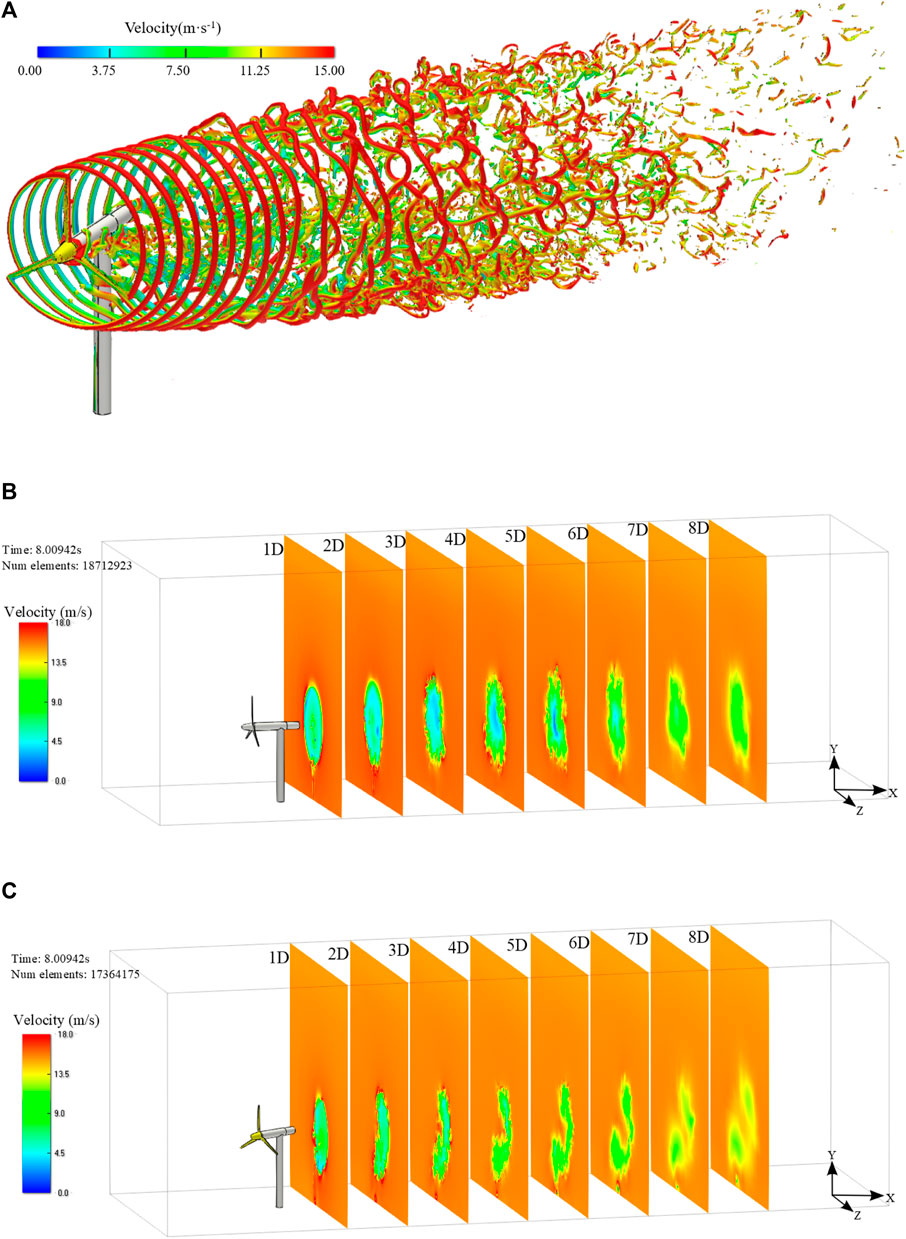
FIGURE 8. Instantaneous contour: (A) Wake structure behind the wind turbine under ϒ = 30°; (B) Velocity contour of the different vertical section under ϒ = 0°; (C) Velocity contour of the different vertical section under ϒ = 30°.

Rapid Dynamic Yaw

In this study, first, we keep the wind turbine in operation without yaw until a stable wake state is established, and then the dynamic yaw of the wind turbine continues. In the simulation, the wind turbine maintains a non-yaw state from t = 0 s to 200 s when a stable flow field is obtained through the development. As shown in the instantaneous vorticity contour of the horizontal section at the hub height under the rapid yaw in Figure 9, the wind turbine begins to yaw rapidly from t = 200 s (ϒ = 0°), and only the tip vortices of the first three turns are deflected at t = 206 s (ϒ = 30°). At t = 225 s (ϒ = 30°), all the tip vortex structures in regular shape are deflected, and the broken vortices in the far wake region remain in their original positions. In the horizontal direction, the tip vortex system deforms due to the inductive effect of uneven yaw states. The interaction after the deformation of the tip vortex causes a local inductive vortex system. Compared with ϒ = 0°, the tip vortex is unstable, resulting in the fact that instability and brokenness occur early. In the meantime, the dissipation of the vortex also occurs in the root, distributing small vortex structures with less vorticity strength. At t = 250 s (ϒ = 30°), the deflected tip vortexes turn unstable, and break into small-scale vortexes developing downwards, and many dissipative vortexes without yawing in the far wake region did not disappear. The structure of three-dimensional vorticity at t = 300 s and t = 400 s, respectively, are similar. However, the number of mesh elements continues to increase, and the wake caused by the rapid dynamic yaw has not yet fully developed. Compared with the wake vorticity field without yawing at t = 200 s, the radial width of the wake becomes narrower when the deflection of the wake occurs at t = 400 s, and the tip vortex of the wake is broken in advance. Due to the rapid change of the yaw, the near wake quickly deflects in the yaw direction, while the far wake has not yet deflected due to the delay of the wake (Figure 10; Time 225 s and 250 s).

FIGURE 9

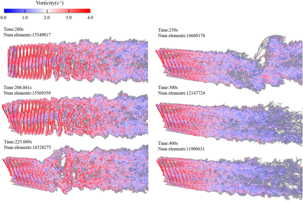
FIGURE 9. Instantaneous vorticity contour of the horizontal section at the hub height under the rapid dynamic yaw.

FIGURE 10

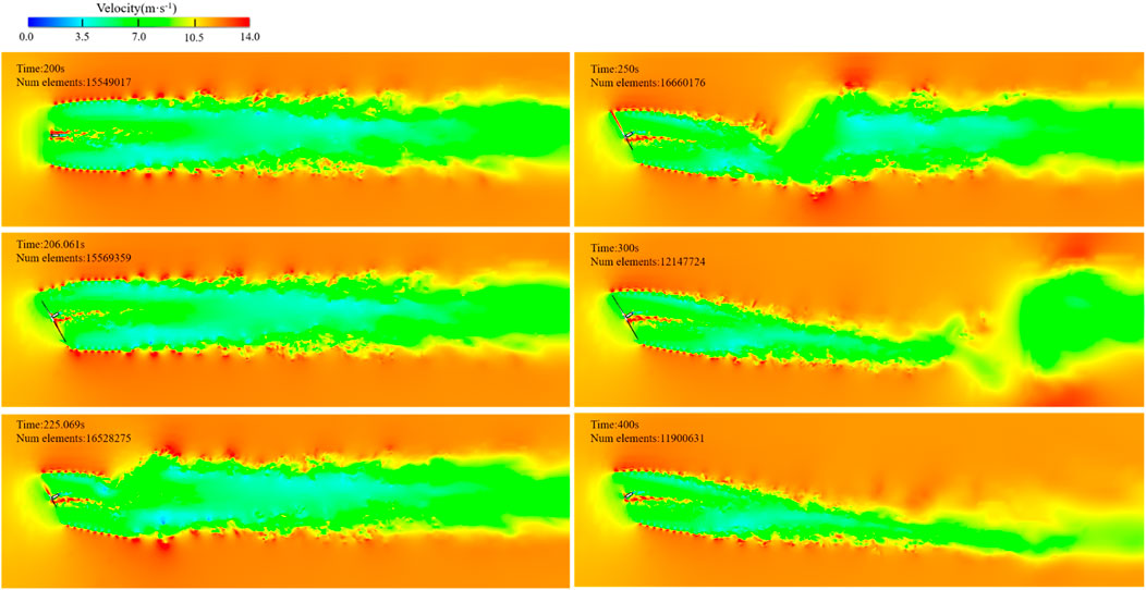
FIGURE 10. Instantaneous velocity contour of the horizontal section at the hub height under the rapid dynamic yaw.

The instantaneous velocity contour of the horizontal section at the hub height under the rapid dynamic yaw is shown in Figure 10. After the rapid dynamic yaw at t = 206 s (ϒ = 3ׄ0°), only the velocity near the rotor changes. At t = 225 s, the wake is reversely offset from the yaw angle of the wind turbine, with a large angle deflection of the above wake trace. The above wake trace offset, as the width of the yawing wake is narrowed at t = 250 s. The structure of three-dimensional vorticity at t = 300 s and t = 400 s, respectively, are similar, but the velocity change in the far wake region is delayed. At t = 400 s, the wake velocity caused by the yawing has been fully developed. Compared with the wake velocity field of ϒ = 0°, the wake shows a large angle deflection, and the width of the core area of the wake velocity loss becomes narrower. In addition, the deceleration zone decreases, and the wake recovery velocity becomes faster. The deflection of the wake is difficult to predict, which can be simply implied by the conservation of momentum, that is, the wind turbine exerts a lateral force on the airflow, thereby producing a rotating wake velocity. Bastankhah and Porté-Agel (2016) performed wind tunnel experiments to measure the yaw wake information and used it for budget studies on the continuity and the RANS equations of the yaw turbine wake, their theoretical analysis revealed that the wake velocity recovered faster on the side of the larger wake skew angle, indicating that the wake will move to the opposite side when moving downstream. The rapid dynamic yaw is completed within 6 s, and the near wake skew angle is asymmetrically distributed with a large difference, resulting in wake deflection in the same direction as the yaw. However, the deflection angle of the far wake remains unchanged and symmetrically distributed due to the wake delay, and the transition zone between the far wake and the near wake deviates significantly, which is opposite to the yaw direction.

Slow Dynamic Yaw

In order to obtain the information during the slow dynamic yaw process, first, we performed the simulation of the turbine without yaw until the wake developed to a stable state, and then continue with the slow dynamic yaw of the wind turbine. In the simulation, the wind turbine maintains a non-yaw state from t = 0 s, and 150 s. It can be seen from Figure 11 that the wind turbine yaws at a speed of 0.3°/s from t = 150 s. When t = 200 s and ϒ = 15°, the root vortex is no longer concentrated in the center of the range surrounded by the spiral tip vortex, but dissipates into many small vortexes, and the deflection of the wake vortex is not obvious. When t = 250 s, and ϒ= 30°, the tip vortex of the wake is broken in advance, the width of the near wake is narrowed, and the wake shows no large-angle deflection. Moreover, the wake is reversely offset from the yaw angle of the wind turbine. When t = 300 s and ϒ= 45°, the slow dynamic yaw is completed. During the slow dynamic yaw process, the distance between the breaking position of the tip vortex and the wind turbine becomes longer, and the continuous distance of the tip vortex structure downstream becomes longer. At t = 400 s, the wake with ϒ = 45° develops for 100 s, the radial width of the wake becomes narrower, and the regular tip vortex structure further develops downstream. In addition, the tip vortex structure can still be observed at the 3D position behind the wind turbine. The instantaneous vorticity at t = 600 s and t = 400 s are similar, and the number of num elements no longer increases, therefore, the wake has been fully developed after t = 400 s. In the process of the slow dynamic yaw, the far wake deflects in the same direction as the yaw.

FIGURE 11

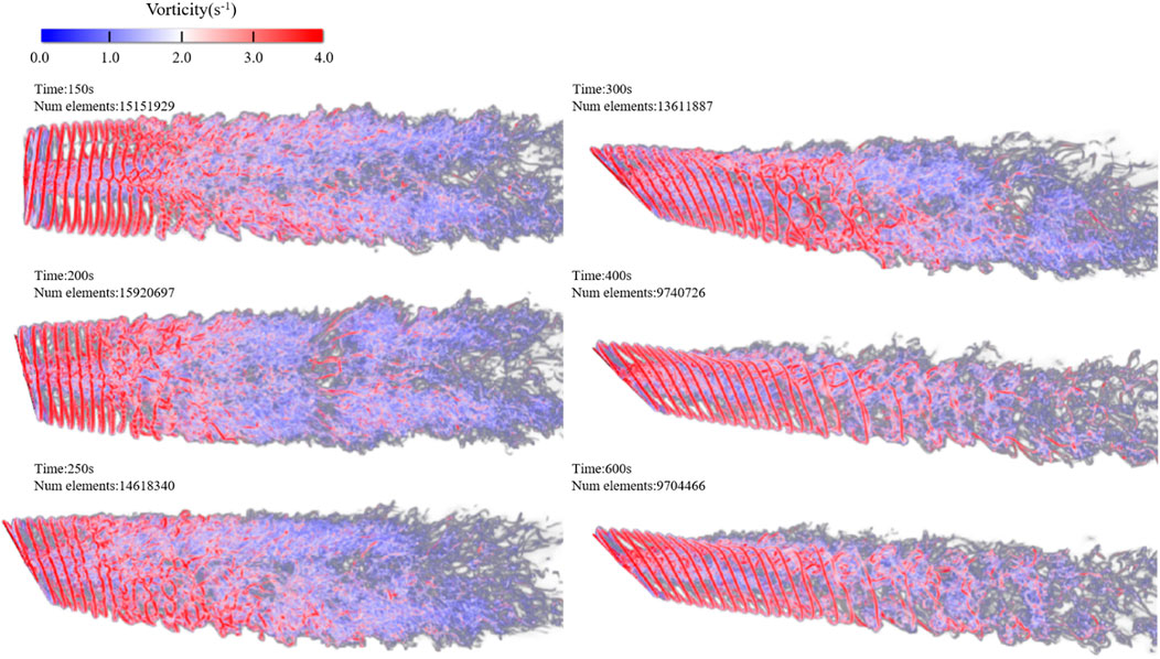
FIGURE 11. Instantaneous vorticity contour of the horizontal section at the hub height under the slow dynamic yaw.

Figure 12 illustrates the instantaneous velocity contour of the horizontal section at the hub height under the slow dynamic yaw. The wake recovery is mainly affected by the incoming turbulence, and the wake deflection increases with the decrease of the incoming turbulence (Vermeulen, 1980). Bastankhah and Porté-Agel (2016) pointed out that the wake width in the far wake region changes approximately linearly in the experimental study, the wake growth rate k is similar (k = 0.022) for different steady yaw angles. The slow dynamic yaw is completed within 150 s. At the completion of the yaw (t = 300 s), the wake affected by the yaw begins to pass through the outlet of the calculation domain. During the calculation of the slow dynamic yaw, the ambient turbulence remains unchanged, while the yaw angle changes slowly. Therefore, the wake can maintain a continuous deflection with a similar wake growth rate. In comparison with the rapid dynamic yaw, the transition wake region does not show an obvious deflection. The horizontal width of the wake center of the low-speed core area in the near wake begins to narrow at t = 300 s, which is quite different from the velocity distribution in the far wake region of the rapid dynamic yaw (Figure 10, t = 206 s). At t = 400 s, the wake of the slow dynamic yaw is fully developed, and the width of the core area of the wake velocity in the far wake is further narrowed. However, it can be seen from Figure 11 that the far wake continues to spread and develop, gradually mixing with the surrounding flow.

FIGURE 12

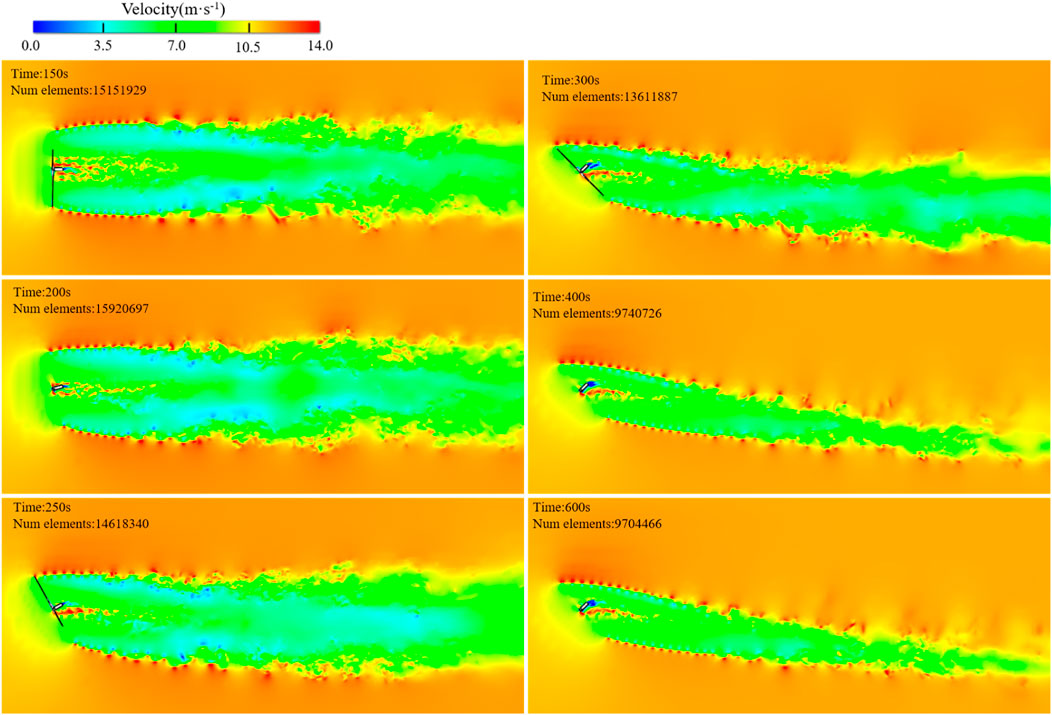
FIGURE 12. Instantaneous velocity contour of the horizontal section at the hub height under the slow dynamic yaw.

As shown in Figures 10, 12, the wake narrows in dynamic yaw situations. The instantaneous velocity contours of the wake cross-section at 0.5D and 5D behind the turbine rotor are shown in Figure 13, during the dynamic yaw process, the horizontal width of the near wake (0.5D) gradually narrows, and the vertical height increases slowly. However, the development of the far wake area (5D) is lagging due to the dynamic yaw. As the yaw wake develops, the far wake forms a cross-section in kidney shape, which is consistent with the steady yaw. The wake distributed in the horizontal direction is narrower than that in the vertical direction. As shown in the analytical model (Howland et al., 2016) for the yaw wake, the wake width changes linearly in the streamwise direction at a stable yaw angle. However, during the dynamic yaw process, the yaw angle continues to change with the similar wake expansion (Howland et al., 2016), and the lateral width of the wake during the dynamic yaw process changes with the changes of x and ϒ. The prediction result of the model (ϒ = ϒ′) is equivalent to the time-varying dynamic wake produced by the wind turbine when the dynamic yaw angle is ϒ′.

FIGURE 13

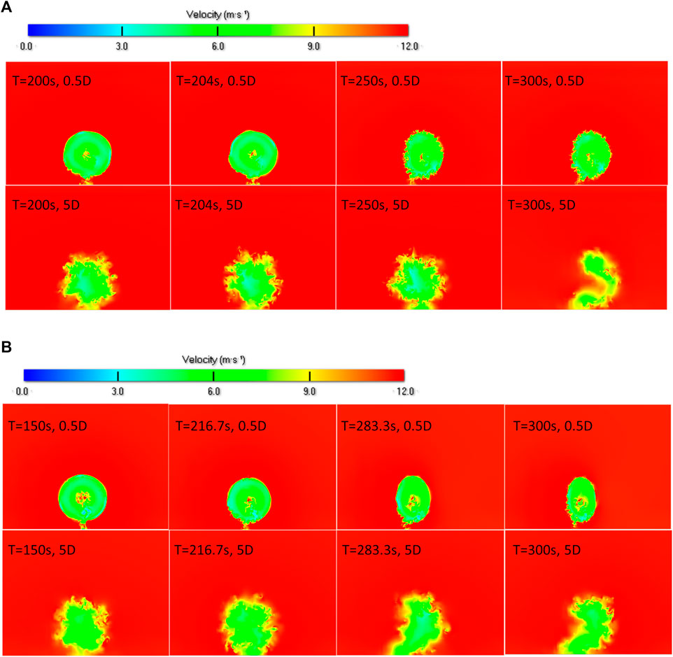
FIGURE 13. The instantaneous velocity contours of the wake cross-section at 0.5D and 5D behind the turbine rotor: (A) rapid dynamic yaw; (B) slow dynamic yaw.

Bastankhah derived an analytical model for the yaw wake (Bastankhah and Porté-Agel, 2016):

$\frac{△\overline{u}}{u_{\infty }}=\left(1-\sqrt{1-\frac{C_T\cos \gamma }{8({\delta }_y{\delta }_z/D^2)}}\right){\text{e}}^{-0.5{\left((y-\delta )/{\delta }_y\right)}^2}{\text{e}}^{-0.5{\left((z-z_h)/{\delta }_z\right)}^2}(18)$

$\{\begin{array}{l}{\delta }_y=k(x-x_0)+\frac{D\cos \gamma }{\sqrt{8}}\\ {\delta }_z=k(x-x_0)+\frac{D}{\sqrt{8}}\end{array}(19)$

where $u_{\infty }$ is the free inflow velocity, $△\overline{u}$ is the velocity deficit, ${\delta }_y$ is the wake widths in the lateral direction, ${\delta }_z$ is the wake widths in the vertical direction, $C_T$ is the thrust coefficient, D is the diameter of the turbine, ϒ is the yaw angle, σ is the value of the wake deflection, and $z_h$ is the hub height of the turbine.

The calculation results of steady yaw wake velocity at different axial distances of the hub height are compared with the results of Bastankhah’s model (Bastankhah and Porté-Agel, 2015) are shown in Figure 14. It can be found that the wake without yaw is distributed symmetrically along the centerline (Z/D = 0) of the hub. With the steady yaw wake developing downstream, the degree of skew continuously increases, and the width of the wake continuously narrows. The velocity profiles at the hub height show an approximate symmetry along different lines (The symmetrical centerline Z/D increases as the wake flows downstream) at different axial locations. In the far wake, the wake recovery speed of the yaw condition is faster than that when ϒ = 0°. In the yaw condition, the wake velocity is recovered at an 8D distance behind the wind turbine, and the loss of wake velocity under ϒ = 45° is less than that under ϒ = 30°. This is consistent with the conclusion that the wake deflection increases with the increase of the yaw angle (Abkar and Porté-Agel, 20151994). As the airflow passes through the yaw rotor, the core area of the wake is not affected by the environmental flow, therefore, the flow angle and velocity of the wake center will not change the potential core. As it develops downstream, the potential core of the wake will change, making it smaller until it ends after about 4D (Figure 14 4D). Then the center of the wake begins to recover, and the far wake diffuses and develops continuously. The numerical simulation results are more consistent with the prediction results of the model (Bastankhah and Porté-Agel, 2015) after the 5D distance, and the core area of the far wakes predicted by the two models are relatively close. However, the wind speed distributions predicted by the two models are quite different in the near wake region, the prediction of Bastankhah’s wake model is not very accurate, which simplifies the near-wake velocity distribution curve, and the LBM simulated near-wake velocity distribution is still a bimodal structure. For higher yaw angles (γ > 30°), the prediction of Bastankhah’s model is not very accurate either, which may be due to the assumption that the wake velocity profile has a symmetrical Gaussian distribution. In addition, it is shown that the velocity profile is slightly inclined.

FIGURE 14

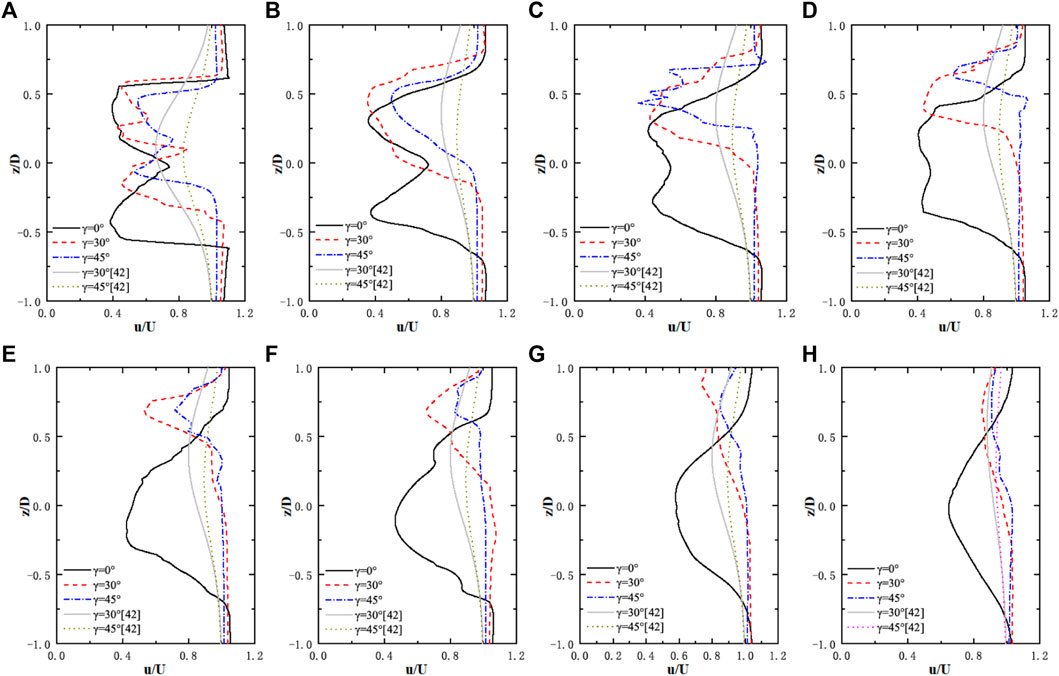
FIGURE 14. Calculation results of wake velocity in yaw at different axial distances of the hub height compared with the prediction results of Bastankhah’s analytical model (Bastankhah and Porté-Agel, 2016). [The gray solid line and the dotted line are the prediction results of the yaw wake model (Bastankhah and Porté-Agel, 2016)]: (A) 1D; (B) 2D; (C) 3D; (D) 4D; (E) 5D; (F) 6D; (G) 7D; (H) 8D.

As shown in Figure 15, the thrust of the wind turbine before the rapid dynamic yaw oscillates up and down at around 805 kN, and the rapid dynamic yaw starts from 200 s, when the thrust drops rapidly. When the yaw is stabilized at 30°, the axial thrust oscillates up and down around 600 kN, the axial thrust is reduced by 25.4%. The slow dynamic yaw starts to yaw from t = 150 s, and the axial thrust gradually decreases (non-linear change). When the yaw stabilizes at 45°, the axial thrust oscillates up and down at 410 kN, and the axial thrust drops by 46.8%. Since the NREL 5 MW wind turbine has a three-bladed structure, the wind turbine experiences a drop in thrust when one blade passes by the tower, which is observed three times per rotor revolution at the azimuth angles of 60+, 180+, and 300+, respectively. With the increase of the yaw angle, the time point of the thrust drop is delayed.

FIGURE 15

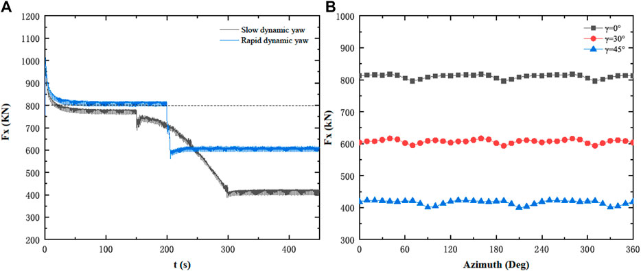
FIGURE 15. Evolution of aerodynamic thrust: (A) thrust over simulation time; (B) in the last simulated rotation (At 0+ azimuth, Blade 1 points vertically up).

In the actual turbulent conditions, the recovery speed of the yaw wake will increase. It can also be seen from formula 18 that the wake widths will increase with the increase in k (wake expansion coefficient increases with the turbulence intensity). In the experiment, it is found that the wake deflection decreases with the increase of turbulence (Vermeulen, 1980). Therefore, under actual turbulence conditions, the deflection in the transition zone between the far wake and the near wake in the rapid yaw process will decrease, while in the slow dynamic yaw, the far wake deflects relatively forward to the yaw. The cross-section of the yaw wake will still be kidney-shaped, the horizontal wake distribution is narrower than the vertical direction, and the actual turbulence will aggravate the asymmetric distribution of the yaw wake.

Conclusion

The LBM-LES method was applied to the simulations of the yawed MEXICO wind turbine, and the calculated results were compared with the experimental values. The NREL 5 MW offshore wind turbine was used to analyze the wake characteristics of a rapid and a slow dynamic yaw operation. Conclusions are drawn as follows:

1) The calculated values of the velocity distributions along the axial and radial directions at different positions in the near wake area are in good agreement with the experimental values. In the far wake area, the wake forms a cross-section in kidney shape, and the wake distributed in the horizontal direction is narrower than that in the vertical direction. The LBM-LES method is reliable for the unsteady wake calculation of wind turbines under the yaw.

2) During the rapid dynamic yaw, the transition area between the far wake and the near wake shows a large deflection, and the transition zone deviates significantly, which is opposite to the yaw direction. However, in the process of the slow dynamic yaw, the far wake deflects forward relatively to the yaw. During the yaw process, the wake skews as it develops downstream, the far wake forms a cross-section in kidney shape consistent with that in the steady yaw, and the wake distributed in the horizontal direction is narrower than that in the vertical direction. The wake recovery speed of the yaw condition is greater than the one in the case without yaw.

3) At the beginning of the slow dynamic yaw, the unevenness in the horizontal direction causes the deformation of the tip vortex system, and the tip vortex is unstable. The tip vortex becomes unstable, and breaks earlier in comparison with the case without yaw. The increase of the yaw angle results in a longer length of the spiral blade tip vortex downstream of the wind, and the tip vortex becomes unstable and fragmented later.

4) Under the rated conditions, the thrust of the NREL 5 MW wind turbine fluctuates around 800 kN. When the wind turbine yaws rapidly, the thrust drops largely. However, when it yaws slowly, the dropping of thrust becomes slow. At the yaw angle of 30°, the mean thrust is reduced by 25.4%, and when the yaw angle is 45°, the mean thrust is reduced by 46.8%. The thrust of the wind turbine experiences a drop three times per rotor revolution at the azimuth angles of 60+, 180+, and 300+, respectively, when one blade passes by the tower. The increase of the yaw angle leads to the delayed time of thrust dropping.

Data Availability Statement

The raw data supporting the conclusion of this article will be made available by the authors, without undue reservation.

Author Contributions

FX: formal analysis, investigation, data curation and writing. CX: methodology, writing—review and editing, and funding acquisition. HH: analysis, investigation and data curation. WS: supervision and writing—review and editing. XH: conceptualization and supervision. ZJ: writing—review and editing.

Funding

This research was supported by the Research on smart operation control technologies for offshore wind farms (Grant No. 2019YFE0104800); National Science Foundation of China-Yalong River Joint Fund (Grant No. U1865101); Fundamental Research Funds for the Central Universities (Grant No. B200203057); Postgraduate Research & Practice Innovation Program of Jiangsu Province (Grant No. KYCX20_0470); and Priority Academic Program Development of Jiangsu Higher Education Institutions.

Conflict of Interest

HH was employed by Power China Hua Dong Engineering Corporation Limited.

The remaining authors declare that the research was conducted in the absence of any commercial or financial relationships that could be construed as a potential conflict of interest.

Publisher’s Note

All claims expressed in this article are solely those of the authors and do not necessarily represent those of their affiliated organizations, or those of the publisher, the editors, and the reviewers. Any product that may be evaluated in this article, or claim that may be made by its manufacturer, is not guaranteed or endorsed by the publisher.

References

Abkar, M., and Porté-Agel, F. (2015). Influence of Atmospheric Stability on Wind-Turbine Wakes: A Large-Eddy Simulation Study. Phys. Fluids 27 (3), 035104. doi:10.1063/1.4913695

CrossRef Full Text | Google Scholar

Bastankhah, M., and Porté-Agel, F. (2015). A Wind-Tunnel Investigation of Wind-Turbine Wakes in Yawed Conditions. J. Phys. Conf. Ser. 625 (1), 012014. doi:10.1088/1742-6596/625/1/012014

CrossRef Full Text | Google Scholar

Bastankhah, M., and Porté-Agel, F. (2016). Experimental and Theoretical Study of Wind Turbine Wakes in Yawed Conditions. J. Fluid Mech. 806, 506–541. doi:10.1017/jfm.2016.595

CrossRef Full Text | Google Scholar

Boorsma, K., and Schepers, J. G. (2014). New MEXICO experiment. Petten, Netherlands: Energy Research Centre of the Netherlands. ECN-E-14-048.

Google Scholar

Chapman, S., and Cowling, T. G. (1970). The Mathematical Theory of Non-uniform Gases. 3rd edition. Cambridge University Press.

Google Scholar

Chen, L., Yu, Y., Lu, J., and Hou, G. (2014). A Comparative Study of Lattice Boltzmann Methods Using Bounce-Back Schemes and Immersed Boundary Ones for Flow Acoustic Problems. Int. J. Numer. Meth. Fluids 74 (6), 439–467. doi:10.1002/fld.3858

CrossRef Full Text | Google Scholar

Cheng, H., Qiao, Y., Liu, C., Li, Y., Zhu, B., Shi, Y., et al. (2012). Extended Hybrid Pressure and Velocity Boundary Conditions for D3Q27 Lattice Boltzmann Model. Appl. Math. Model. 36 (5), 2031–2055. doi:10.1016/j.apm.2011.08.015

CrossRef Full Text | Google Scholar

Cortina, G., Sharma, V., and Calaf, M. (2017). Investigation of the Incoming Wind Vector for Improved Wind Turbine Yaw-Adjustment under Different Atmospheric and Wind Farm Conditions. Renew. Energ. 101, 376–386. doi:10.1016/j.renene.2016.08.011

CrossRef Full Text | Google Scholar

Dai, J., Yang, X., Hu, W., Wen, L., and Tan, Y. (2018). Effect Investigation of Yaw on Wind Turbine Performance Based on SCADA Data. Energy 149, 684–696. doi:10.1016/j.energy.2018.02.059

CrossRef Full Text | Google Scholar

Deiterding, R., and Wood, S. L. (2016). An Adaptive Lattice Boltzmann Method for Predicting Wake fields behind Wind Turbines. Springer International Publishing, 845–857. doi:10.1007/978-3-319-27279-5_74

CrossRef Full Text | Google Scholar

Deiterding, R., and Wood, S. L. (2016). Predictive Wind Turbine Simulation with an Adaptive Lattice Boltzmann Method for Moving Boundaries. J. Phys. Conf. Ser. 753 (8), 082005. doi:10.1088/1742-6596/753/8/082005

CrossRef Full Text | Google Scholar

Di Ilio, G., Chiappini, D., Ubertini, S., Bella, G., and Succi, S. (2018). Fluid Flow Around NACA 0012 Airfoil at Low-reynolds Numbers with Hybrid Lattice Boltzmann Method. Comput. Fluids 166, 200–208. doi:10.1016/j.compfluid.2018.02.014

CrossRef Full Text | Google Scholar

Dong, Y.-H., and Sagaut, P. (2008). A Study of Time Correlations in Lattice Boltzmann-Based Large-Eddy Simulation of Isotropic Turbulence. Phys. Fluids 20, 035105. doi:10.1063/1.2842381

CrossRef Full Text | Google Scholar

Hähnel, D. (2004). Molekulare Gasdynamik. Germany: Springer-Verlag Berlin Heidelberg.

Google Scholar

Han, X., Liu, D., Xu, C., and Shen, W. Z. (2018). Atmospheric Stability and Topography Effects on Wind Turbine Performance and Wake Properties in Complex Terrain. Renew. Energ. 126, 640–651. doi:10.1016/j.renene.2018.03.048

CrossRef Full Text | Google Scholar

Howland, M. F., Bossuyt, J., Martínez-Tossas, L. A., Meyers, J., and Meneveau, C. (2016). Wake Structure in Actuator Disk Models of Wind Turbines in Yaw under Uniform Inflow Conditions. J. Renew. Sust. Energ. 8 (4), 043301. doi:10.1063/1.4955091

CrossRef Full Text | Google Scholar

Jensen, N. O. (1983). A Note on Wind Generator Interaction. Copenhagen, Roskilde, Denmark: Risø National LaboratoryRoskilde, Denmark. 87-550-0971-9.

Google Scholar

Jiménez, Á., Crespo, A., and Migoya, E. (2010). Application of a LES Technique to Characterize the Wake Deflection of a Wind Turbine in Yaw. Wind Energ. 13 (6), 559–572. doi:10.1002/we.380

CrossRef Full Text | Google Scholar

Jing, B., Qian, Z., Pei, Y., Zhang, L., and Yang, T. (2020). Improving Wind Turbine Efficiency through Detection and Calibration of Yaw Misalignment. Renew. Energ. 160, 1217–1227. doi:10.1016/j.renene.2020.07.063

CrossRef Full Text | Google Scholar

Kaoui, B. (2020). Algorithm to Implement Unsteady Jump Boundary Conditions within the Lattice Boltzmann Method. Eur. Phys. J. E 43 (4), 23. doi:10.1140/epje/i2020-11947-x

PubMed Abstract | CrossRef Full Text | Google Scholar

Khan, A. (2018). Finite Element Analysis of Aerodynamic Coefficients of a HAWT Blade Using LBM Method. ICOME. doi:10.1063/1.5044317

CrossRef Full Text | Google Scholar

Kim, M. S., Franck, P., and Meskine, M. (2012). ISROMAC 2012 - 14th International Symposium on Transport Phenomena and Dynamics of Rotating Machinery.

Google Scholar

Kress, C., Chokani, N., and Abhari, R. S. (2015). Downwind Wind Turbine Yaw Stability and Performance. Renew. Energ. 83, 1157–1165. doi:10.1016/j.renene.2015.05.040

CrossRef Full Text | Google Scholar

Leble, V., and Barakos, G. (2017). 10-MW Wind Turbine Performance under Pitching and Yawing Motion. J. Sol. Energ. Eng. 139, 041003. doi:10.1115/1.4036497

CrossRef Full Text | Google Scholar

Li, L., Ding, W., Xue, F., Xu, C., and Li, B. (2018). Multiscale Mathematical Model with Discrete-Continuum Transition for Gas-Liquid-Slag Three-phase Flow in Gas-Stirred Ladles. Jom 70 (12), 2900–2908. doi:10.1007/s11837-018-3116-5

CrossRef Full Text | Google Scholar

Li, L., Xu, C., Shi, C., Han, X., and Shen, W. (2020). Investigation of Wake Characteristics of the MEXICO Wind Turbine Using Lattice Boltzmann Method. Wind Energy 24 (2), 116–132. doi:10.1002/we.2560

CrossRef Full Text | Google Scholar

Macrí, S., Aubrun, S., Leroy, A., and Girard, N. (2021). Experimental Investigation of Wind Turbine Wake and Load Dynamics during Yaw Maneuvers. Wind Energ. Sci. 6 (2), 585–599. doi:10.5194/wes-6-585-2021

CrossRef Full Text | Google Scholar

Nejad, A. R., Guo, Y., Gao, Z., and Moan, T. (2016). Development of a 5 MW Reference Gearbox for Offshore Wind Turbines. Wind Energy 19, 1089–1106. doi:10.1002/we.1884

CrossRef Full Text | Google Scholar

Nicoud, F., and Ducros, F. (1999). Subgrid-scale Stress Modelling Based on the Square of the Velocity Gradient Tensor. Flow, Turbulence and Combustion 62 (3), 183–200. doi:10.1023/A:1009995426001

CrossRef Full Text | Google Scholar

Pereira, R., Schepers, G., and Pavel, M. D. (2013). Validation of the Beddoes-Leishman Dynamic Stall Model for Horizontal axis Wind Turbines Using MEXICO Data. Wind Energ. 16 (2), 207–219. doi:10.1002/we.541

CrossRef Full Text | Google Scholar

Qian, Y. H., D'Humières, D., and Lallemand, P. (1992). Lattice Bgk Models for Navier-Stokes Equation. Europhys. Lett. 17 (6BIS), 479–484. doi:10.1209/0295-5075/17/6/001

CrossRef Full Text | Google Scholar

Qiu, Y.-X., Wang, X.-D., Kang, S., Zhao, M., and Liang, J.-Y. (2014). Predictions of Unsteady HAWT Aerodynamics in Yawing and Pitching Using the Free Vortex Method. Renew. Energ. 70, 93–106. doi:10.1016/j.renene.2014.03.071

CrossRef Full Text | Google Scholar

Rullaud, S., Blondel, F., and Cathelain, M. (2018). Actuator-line Model in a Lattice Boltzmann Framework for Wind Turbine Simulations. J. PhysicsConference Ser. 1037 (2), 22023. doi:10.1088/1742-6596/1037/2/022023

CrossRef Full Text | Google Scholar

Snel, H., Schepers, J. G., and Montgomerie, B. (2007). The MEXICO Project (Model Experiments in Controlled Conditions): The Database and First Results of Data Processing and Interpretation. J. Phys. Conf. Ser. 75, 012014. doi:10.1088/1742-6596/75/1/012014

CrossRef Full Text | Google Scholar

Vashahi, F., and Lee, J. (2018). On the Emerging Flow from a Dual-Axial Counter-rotating Swirler; LES Simulation and Spectral Transition. Appl. Therm. Eng. 129, 646–656. doi:10.1016/j.applthermaleng.2017.10.058

CrossRef Full Text | Google Scholar

Vermeulen, P. E. J. (1980). “An Experimental Analysis of Wind Turbine Wakes,” in 3rd International Symposium on Wind Energy Systems (Copenhagen, Denmark: Lyngby), 431–450.

Google Scholar

Wang, X., Ye, Z., Kang, S., and Hu, H. (2019). Investigations on the Unsteady Aerodynamic Characteristics of a Horizontal-axis Wind Turbine during Dynamic Yaw Processes. Energies 12 (16), 3124. doi:10.3390/en12163124

CrossRef Full Text | Google Scholar

Wen, B., Tian, X., Dong, X., Peng, Z., Zhang, W., and Wei, K. (2019). A Numerical Study on the Angle of Attack to the Blade of a Horizontal-axis Offshore Floating Wind Turbine under Static and Dynamic Yawed Conditions. Energy 168, 1138–1156. doi:10.1016/j.energy.2018.11.082

CrossRef Full Text | Google Scholar

Wood, S. L., and Deiterding, R. (2015). A Lattice Boltzmann Method for Horizontal Axis Wind Turbine Simulation, In 14th International Conference on Wind Engineering. Brazil, 21–26. Corpus ID: 2952897.

Google Scholar

Wu, W., Liu, X., Dai, Y., and Li, Q. (2020). An In-Depth Quantitative Analysis of Wind Turbine Blade Tip Wake Flow Based on the Lattice Boltzmann Method. Environ. Sci. Pollut. Res. 28 (30), 40103–40115. doi:10.1007/s11356-020-09511-8

CrossRef Full Text | Google Scholar

Xu, J. (2016). Wake Interaction of NREL Wind Turbines Using a Lattice Boltzmann Method. Sust. Energ. 4, 1–6. doi:10.12691/RSE-4-1-1

CrossRef Full Text | Google Scholar

Ye, Z., Wang, X., Chen, Z., and Wang, L. (2020). Unsteady Aerodynamic Characteristics of a Horizontal Wind Turbine under Yaw and Dynamic Yawing. Acta Mech. Sin. 36 (2), 320–338. doi:10.1007/s10409-020-00947-2

CrossRef Full Text | Google Scholar

Yuan, H. Z., Wang, Y., and Shu, C. (2017). An Adaptive Mesh Refinement-Multiphase Lattice Boltzmann Flux Solver for Simulation of Complex Binary Fluid Flows. Phys. Fluids 29 (12), 1236041–12360416. doi:10.1063/1.5007232

CrossRef Full Text | Google Scholar

Glossary

LBM Lattice Boltzmann method

LES Large eddy simulation

PIV Particle image velocimetry

NREL National Renewable Energy Laboratory

MEXICO Model Rotor Experiment in Controlled Conditions

WALE Wall-Adapting Local Eddy

AMR Adaptive mesh refinement

CVP Counter-rotating vortex pair

x, y, z three-dimensional coordinates with the origin placed at the hub center of the wind turbine

x′, y′, z′ spatial coordinates in the actual flow field

ξ velocity of the particle

N the kind of velocity

f continuous distribution function

r point

t time

e_α the corresponding discrete velocity the discrete velocity

F_α external force in the discrete velocity space

M the problem dimension 27 × 27 matrix

n the number of lattice chains

ρ fluid density

ω_α the density weighting factor

u the macroscopic velocity

c_s the lattice sound velocity

e_α the corresponding discrete velocity the discrete velocity

σ_x lattice step

σ_t time step

c the lattice migration rate

$\overline{\varphi }$ the large-scale average component

${\varphi }^{\prime }$ the small-scale component

D flow area

x′ the spatial coordinate in the actual flow field

u_i the speed in i direction

μ the dynamic viscosity

τ_ij the sub-grid scale stress

C_W the WALE model constant, 0.2

$S_{ij}^d$ the traceless symmetric part of the square of the velocity gradient tensor

S the collision matrix

M the problem dimension 27 × 27 matrix

$u_{\infty }$ free inflow velocity

$△\overline{u}$ the velocity deficit

${\delta }_y$ the wake width in the lateral direction

${\delta }_z$ the wake width in the vertical direction

$C_T$ the thrust coefficient

ϒ the yaw angle

σ the value of wake deflection

$z_h$ the hub height of the turbine