 Yuchuan Guo
 Zilin Su
 Zeguang Li
 Kan Wang
94% of researchers rate our articles as excellent or good
Learn more about the work of our research integrity team to safeguard the quality of each article we publish.
Find out more
ORIGINAL RESEARCH article
Front. Energy Res., 27 January 2022
Sec. Nuclear Energy
Volume 10 - 2022 | https://doi.org/10.3389/fenrg.2022.819033
This article is part of the Research TopicExperimental and Analytical Investigations on Nuclear Reactor Safety, Severe Accident Phenomena and Severe Accident Mitigation of Nuclear Power PlantsView all 20 articles
Differing from the traditional Pressurized Water Reactor (PWR), heat pipe cooled reactor adopts the high-temperature heat pipes to transport fission heat generated in the reactor core. Therefore, the basis of coupling calculation on this type of reactor system is to have a suitable model for high-temperature heat pipe simulation. Not only is it required that this model can well describe the transient characteristics of heat pipe, but it should be simple enough to reduce the computational resource. In this paper, the super thermal conductivity model (STCM) for high-temperature heat pipe is proposed for this purpose. In this model, heat transport of vapor flow is simplified as high efficiency heat conductance. Combined with the network method, the evaporation rate, the condensation rate, and the flow rate in the wick region can be preliminarily obtained. Using recommended equations to calculate the heat transfer limitation, this model can realize the safety judgment of heat pipe. The heating system for high-temperature heat pipe is established to validate this model. The heating experiments with different heating powers is tested. Then, this model is applied on the numerical calculation of Kilowatt Reactor Using Stirling TechnologY (KRUSTY) reactor. In the steady state calculation, the results show that the temperature distribution on contact surface between fuel and heat pipe is nonuniform, which will lead to higher peak temperature and temperature difference for the reactor core. In the transient calculation, the load-following accident is chosen. Comparing with the experimental results, the applicability of the proposed model on heat pipe cooled reactor is verified. This model can be used for heat pipe cooled reactor simulation.
Alkali metal has the characteristics of having a high boiling point and large latent heat of vaporization. Heat pipes using alkali metal can realize efficient heat transport in special environments with high temperature (Faghri, 2014). Wicks with a porous structure can generate an effective pressure head at the vapor-liquid interface, maintaining the stable circulation of working medium (Reay et al., 2013). Due to these characteristics, high-temperature heat pipe is widely used for the design of heat pipe cooled reactor systems. So far, proposed conceptual designs of heat pipe cooled reactor systems include the kilopower reactor system (McClure et al., 2020a), the Heatpipe-Operated Mars Exploration Reactor (HOMER) system (Poston, 2001), and the Heat Pipe-segmented Thermoelectric Module Converters Space Reactor (HP-STMCs) system (El-Genk and Tournier, 2004). This type of reactor system has the advantages of having a compact structure and high safety. It can be used as a mobile nuclear power system or space nuclear system for portable and efficient energy supply (Yan et al., 2020).
Figure 1 shows the basic constitution of a heat pipe cooled reactor (Mcclure, 2015). Heat generated in the reactor core is absorbed by high-temperature heat pipes. Then it is released in the primary heat exchanger through the heat convection between heat pipes and coolant in the secondary system. When the reactor shuts down, decay heat can be taken out of the reactor core through the decay heat exchanger. In general, due to the nonuniformity of reactor power distribution and the directionality of coolant flow in the heat exchanger, the actual heat transport and temperature distribution of each heat pipe are different. Meanwhile, to ensure the safety of heat transport, there are a large number of high-temperature heat pipes in the reactor core. The complex two-phase flow and heat transfer also brings challenges to the numerical calculation of heat pipe. For heat pipe models using the analysis on heat pipe cooled reactors, it is hoped that it can describe the transient behavior of heat pipes well, and it should be simple enough to reduce the computational resources as much as possible.
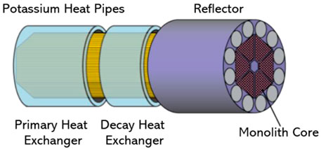
FIGURE 1. Basic constitution of a heat pipe cooled reactor (Mcclure, 2015).
So far, there have been many studies on the numerical analysis of high-temperature heat pipe (Costello et al., 1986; Cao and Faghri, 1991; Cao and Faghri, 1992; Tournier and El-Genk, 1992; Vasiliev and Kanonchik, 1993). Before the 1990s, computing power was limited, so the complex physical phenomena that existed in heat pipe could not be simulated in detail. Therefore, the heat pipe models at this period were based on some reasonable assumptions. For example, the vapor flow in vapor space was assumed to be one-dimensional, while heat conductance in solid region was treated as two-dimensional. The backflow in wick subregion was ignored. During this period, several typical models for heat pipe were put forward successively, including the self-diffusion model (Cao and Faghri, 1993a), the plat-front model (Cao and Faghri, 1993b), the network model (Zuo and Faghri, 1998), and the improved network model (Ferrandi et al., 2013). These models were applied for the simulation of heat pipe cooled reactor (Yuan et al., 2016; Liu et al., 2020; Ma et al., 2020; Wang et al., 2020). However, there are limitations to using these models. For example, the network model cannot consider the nonuniform heat transfer between the heat pipe and the environment. Both the self-diffusion model and the plat-front model consider the two-phase flow and heat transfer in the pipe. During startup, the drastic variation of vapor density, pressure, and velocity may lead to numerical instability.
With the development of high-performance computers, there are more studies on heat pipe simulation using the CFD method (Annamalai and Ramalingam, 2011; Asmaie et al., 2013; Lin et al., 2013; Yue et al., 2018). Using commercial codes such as FLUENT and CFX, the modeling difficulty can be greatly simplified, and built-in advanced numerical algorithms can ensure the stability of numerical calculation as much as possible. The physical processes such as heat conduction, evaporation, condensation, and vapor flow in the heat pipe can be modeled and calculated. CFD modeling and calculation have gradually become the main method for heat pipe analysis. It should be noted that the two-phase flow simulation using CFD method requires large amounts of computing resources. Moreover, for the numerical analysis of heat pipe cooled reactor, more attention should be paid to the heat absorption capability, the temperature variation and distribution, and the operating safety of heat pipe. Phenomena such as vapor flow and vapor-liquid interface shape variation are not important for the safety analysis of heat pipe cooled reactor.
To meet the requirements of heat pipe cooled reactor simulation, the super thermal conductivity model (STCM) is proposed. The heat transport of vapor flow is simplified as high efficiency heat conductance. Combined with the network method, the evaporation, condensation, and backflow can be obtained (Ferrandi et al., 2013). The experimental system for high-temperature heat pipe is established to verify the proposed model. It is then used for the simulation on KRUSTY reactor to discuss the applicability of this model and the characteristics of this type of reactor system.
The model proposed in this paper ignores the two-phase flow and capillary phenomenon in heat pipe, as it simplifies the heat transport caused by vapor flow into high-efficiency heat conductance. Using the network method, the flow of working medium is approximately accounted for. Combined with the recommended heat transfer limitation model (Busse, 1973; Levy, 1968; Deverall et al., 1970; Tien and Chung, 1979), the fast calculation of heat pipe performance and the evaluation of heat pipe safety are realized.
Network model was proposed by Zuo and Faghri (1998); the schematic diagram of this model is shown in Figure 2. Zuo ignored the temperature drop caused by the vapor flow and considered that the temperature drop of the heat pipe was mainly caused by the heat conduction in wall and wick. In addition, Zuo ignored the energy transport caused by the backflow of working medium in wick. Zuo divided the heat pipe into several subregions, and the lumped temperature was used to represent the real temperature of specific subregions. The three-dimensional temperature distribution in each subregion cannot be calculated.
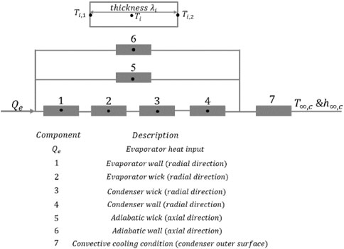
FIGURE 2. The network system for heat pipe operation.
In this paper, the proposed model simplified the heat transport into multi-region heat conduction. The equation that needs to be solved is the differential equation of heat conduction (Eq. 1):
where
For heat pipe, it includes the wall, the wick, and the vapor space. The key to the realization of this model is to determine the thermophysical parameters and heating source of each subregion.
Wall is usually a cylindrical closed shell made of metal. The thermophysical parameters required to solve Eq. 1 are the physical parameters of the corresponding metal. Generally, there is no heat source in wall, and the heat transfer between heat pipe and environment can be described using suitable boundary conditions. Three boundary conditions (Eqs 2–4) can be selected for heat transfer:
where
Wick is composed of a porous structure and liquified working medium. Forms of it include channels, screen, and concentric annulus (Reay et al., 2013). This subregion is usually regarded as the compound material. The thermophysical properties are determined by two materials. For example, for wick with a mesh type, the density, specific heat capacity, and thermal conductivity can be approximately described by Eqs 5–7 (Chi, 1976).
During the operation of heat pipe, liquified working medium in wick will return from condenser to the evaporator. The backflow of working medium is treated as a heating source in a differential equation of heat conduction. Based on the network method, Ferrandi et al. (2013) proposed a simplified method to consider the evaporation, condensation, and backflow (Figure 3). Based on the temperature field calculated at the latest time, the value of each temperature node can be obtained. Combined with the thermal resistance, the evaporation and condensation at vapor-liquid interface can be obtained:
where
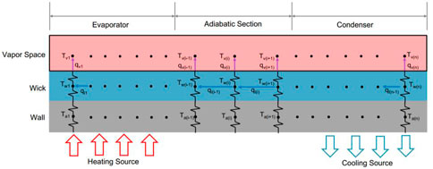
FIGURE 3. Backflow calculation using network model.
Moreover, it is assumed that the fluid circulation is always constant, so backflow in wick can be obtained based on the mass conservation:
Heating source in wick is:
For permeability parameter
For vapor space, the density and specific heat capacity of vapor are the physical parameters of alkali metal (Fink and Leibowitz, 1995; Ohse, 1985; Lee et al., 1969). Therefore, for heat conduction calculation of vapor space, the key is to solve the equivalent thermal conductivity of this subregion.
Firstly, the pressure drops in the evaporator, adiabatic section, and condenser are calculated (Busse, 1967; Reid, 2002; Li et al., 2015).
For evaporator:
The friction coefficient
The axial Reynolds number is:
The velocity profile correction factor
The radial Reynolds number is:
where
For the adiabatic section:
For the condenser:
The velocity profile correction
Combining Eq. 14, Eqs 21–23, the total pressure drop can be determined.
It is assumed that vapor in vapor space and liquified working medium in wick are homogeneous. The Clausius-Clapeyron equation is chosen to describe the relationship between temperature and pressure (Brown, 1951):
Changing Eq. 25 into the differential form:
The heat transfer length along the axial direction is selected as the effective length of heat pipe (Reay et al., 2013):
Combining Fourier’s Law, the equivalent thermal conductivity in vapor space can be obtained:
During the operation of heat pipe, the possible heat transfer limitations include the viscosity limit, the sonic limit, the entrainment limit, and the capillary limit. When the heat transfer limitations occur, the heat transfer capacity of heat pipe will significantly reduce. In this model, the recommended equations for heat transfer limitations are adopted (Busse, 1973; Levy, 1968; Deverall et al., 1970; Tien and Chung, 1979):
During the transient calculation, each limiting power will be calculated using Eqs 29–32. If the calculated value is less than the heating power, the heat transfer limitation will be deemed to occur, and it is assumed that the heat pipe will be damaged. In the future, further numerical analysis and experimental studies will be carried out to investigate the real characteristics of heat pipe when the heat transfer limitation occurs.
To verify the proposed model, a heating system for high-temperature heat pipe is built (Figure 4). It includes the iron-chrome wire heater, the holding device, the angle controlling derive, and the temperature data collection. The iron-chrome wire heater can provide a maximum heating power of 4000 W. To reduce heat leakage as much as possible, the evaporator and the adiabatic section are both wrapped by an insulating layer with aluminum silicate wool.
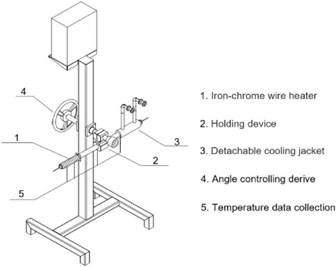
FIGURE 4. Schematic diagram of heating system.
The sodium heat pipe with 1.0 m length is selected as the experiment object. The main parameters of this heat pipe are listed in Table. 1. To ensure the accuracy of temperature data, the groove with 1 mm depth is processed in wall. Using a high-temperature adhesive, all K-type armored thermocouples are fixed in the groove (Figure 5A). Then, they are fixed with the high-temperature adhesive tape. Particularly for the thermocouples in the evaporator, to reduce the effect of heating on temperature measurement, when winding the iron-chrome wire, all the measuring points are bypassed. Ten thermocouples are arranged along the axial direction; the layout position for each thermocouple is shown in Figure 5B.
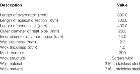
TABLE 1. Parameter description of sodium heat pipe.

FIGURE 5. Heat pipe processing for heating experiments. (A) Grooving processing on heat pipe surface. (B) Temperature sensing point arrangement along the axial direction.
To simplify the experiment, the heat pipe is kept horizontal and is cooled by the natural convection of air. The three-dimensional CFD model of the experimental system is shown in Figure 6, which includes the sodium heat pipe, the electric heater, and the insulating layer. The electric heater is simplified as the thin layer with a thickness of 2 mm, and the heating source is set in this layer as equivalent to an electrical heating. The natural convection between the insulating layer and environment causes heat leakage, and the convective heat transfer coefficient can be determined by Eqs 33, 34. Considering the high temperature of the condenser section, not only the natural convection, but the radiation heat transfer also exist. For radiation of wall, it is treated as the radiant heat transfer to infinite space (Eq. 35).
where
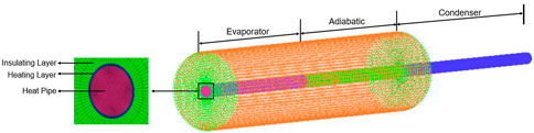
FIGURE 6. Three-dimensional CFD model of the experimental system.
During the experiment, heat pipe is firstly heated to 1200 W to ensure the full startup of heat pipe. Then, the temperature is recorded with the increase of heating power. Figure 7A shows the surface temperature distribution with different heating powers, and Figure 7B shows the temperature variation of heat pipe with time. In these figures, the curve represents the calculated results using this model, and the scatter points represent the results measured by the experiment. According to the comparison, it is found that the temperature calculated by this model differs little from the experimental results. This model can well predict the transient characteristics of high-temperature heat pipe, and the correctness of the proposed model is verified. The difference between two results can be approximately considered to be caused by the uncertainty of parameters used in the model and the uncertainty of the experimental system. Generally, the convective heat transfer coefficient obtained from equation (Eq. 33) is not completely equal to the real value. The uncertainty of boundary conditions will directly lead to the deviation of calculated temperature. Meanwhile, the nonstandard operation during the experiment will also lead to uncertainty of the results. The uncertainty of an experimental system is inevitable. From Figure 7B, it can also be seen that with the continuous increase of heating power, operating temperature of heat pipe will be higher, resulting in the faster response of heat pipe. When heating power is 1600 W, it takes about 13 min to enter the quasi-steady state; when heating power is 3000 W, it takes only about 7 min.
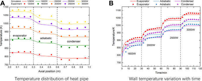
FIGURE 7. Model verification with experimental results. (A) Temperature distribution of heat pipe (B) Wall temperature variation with time.
Figure 8A shows the variation of total temperature difference of heat pipe under the different heating power conditions. When the heating power is low enough, more power leads to the larger temperature difference. This is because that both the temperature drop caused by vapor flow and the temperature gradient caused by heat conduction will increase with the increase of power (Figures 8, 9). When the heating power is high enough, the increase of total temperature difference will become inconspicuous, which means heat pipe has entered the optimal working range. Even if the power is high enough, generated vapor can quickly transport heat to the condenser, meaning the heat pipe shows excellent isothermal property and efficient heat transfer capability.

FIGURE 8. Calculated results using proposed model. (A) Temperature difference with different heating power. (B) Mass flow rate with different heating power.
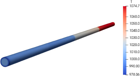
FIGURE 9. Temperature distribution of heat pipe (3000 W).
This model does not directly calculate the vapor flow in the vapor space, however, the evaporation, the condensation, and vapor flow rate can be obtained using the simplified method mentioned in Section 2.2.2. The greater the power, the more evaporation and the greater vapor flow in vapor space. From Figure 8B, it can also be found that although there is an insulating layer wrapped outside the adiabatic section, the high-temperature vapor will still be partially condensed in this section, resulting in the reduction of vapor flow rate in vapor space. It can be predicted that if heat pipe is not well insulated, a considerable part of the heat will be transferred to the environment through the adiabatic section, leading to the decrease in heat transfer efficiency of the heat pipe.
In this section, the proposed model will be used for numerical simulation of KRUSTY reactor. The applicability of this model will be discussed. The characteristics of this reactor are also discussed.
The typical heat pipe cooled reactor named KRUSTY is chosen as the research object. It is the prototype reactor to evaluate the performance of Kilopower reactor system (Poston et al., 2020; Sanchez et al., 2020; McClure et al., 2020b) The composition of KRUSTY reactor is shown in Figure 10. It includes the U-Mo fuel, the BeO reflector, the control rod, the shielding layer, the Na heat pipes, the vacuum vessel, the lift table, and the Stirling generators. The thermal power of the reactor is 5.0 kW. In total, eight sodium heat pipes are used to transport heat to the generators. The Stirling cycle is adopted to generate 1kW electric power. To simplify the modeling, the lift table and support structure are all ignored; only the reactor is established (Figure 11). The Stirling generators are also ignored, the operation of generators is approximated by setting reasonable boundary conditions of the condenser section of heat pipes.
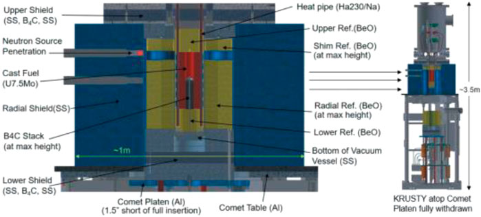
FIGURE 10. Detailed view of the KRUSTY reactor system (Poston et al., 2020).
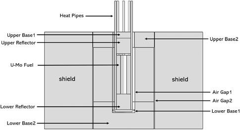
FIGURE 11. Geometric model for KRUSTY reactor.
The outer surface of the reactor always maintains natural convection with the environment. During the steady state analysis (section 4.2), the boundary of the condenser section is set as the fixed temperature. During the load-following analysis (section 4.3), it is set as the fixed temperature gradient.
In this section, the steady state of KRUSTY reactor system is investigated. Both the proposed model in this paper and the network model are adopted. The boundary temperature of the condenser of heat pipes is set as 1,052.0 K, and the fission power is set as 5.0 kW. Figure 12 shows the fuel temperature distribution using the proposed model and network model. For network model, lumped temperature is used to represent the temperature distribution of a specific subregion. Temperature on the contact surface between fuel and heat pipe is always consistent. However, the proposed model can consider the nonuniformity of temperature on contact surface. Compared with the results using network model, the peak temperature of fuel increases from 1,087.6 k to 1,090.8 k, and the total temperature difference increases from 14.4 k to 21.2 k. For KRUSTY reactor, the operation is sensitive to fuel temperature, so the slight variation of temperature may cause an obvious change in fission power. Therefore, it is important for the numerical calculation of heat pipe cooled reactor to obtain the accurate temperature distribution as much as possible. Moreover, for reactor systems with higher power density and more complex heat pipe arrangement, it can be expected that the temperature non-uniform effect of the contact surface will have a more significant impact on the operation of the reactor.
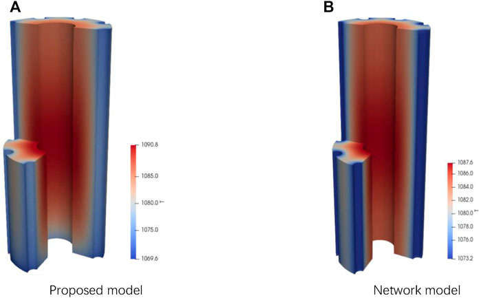
FIGURE 12. Calculated temperature distribution of reactor core. (A) Proposed model. (B) Network model.
The reason for this phenomenon is the uneven power distribution in space. Figure 13 shows the axial distribution of power density obtained by Monte Carlo code RMC. Because of the large aspect ratio of this reactor, the power density presents the distribution of a large value in the middle and a small value on both sides. For reactor systems with a solid attribute, heat conductance is the only way for heat transfer. Based on Fourier’s law, higher heat flux will lead to a larger temperature gradient, resulting in non-uniformity of temperature distribution on the contact surface. It directly affects the actual temperature distribution of the core (Figure 13). From Figures 12–14, it can be concluded that only the three-dimensional modeling of heat pipes and the coupling calculation between heat pipe and the reactor core can obtain the accurate results of heat transfer. The results obtained using the uniform temperature assumption will deviate from the reality.
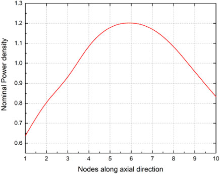
FIGURE 13. Power density distribution along axial distribution.
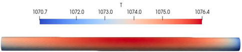
FIGURE 14. Temperature distribution of contact surface between fuel and heat pipe.
In this section, the load-following transient is selected. At T = 0.0 s, the cooling power of the condenser of heat pipe is set as 2.54 kW to represent the decrease of engine power, and the initial fission power is set as 2.67 kW. The difference between the two values is the heat leakage through shield. The comparison between simulated results using the proposed model and experimental results shows in Figure 15. From that, it can be concluded that there is a slight difference between the two results, and proposed model is suitable for the analysis of heat pipe cooled reactor system. On the one hand, to realize the coupling calculation of the heat pipe cooled reactor, the proposed heat pipe model does not directly calculate the working fluid circulation, but adopts a simplified method, which may cause uncertainty to a certain extent. Meanwhile, the detailed information about this experiment is inadequate, and the three-dimensional modeling and the setting of boundary conditions may not be accurate enough.
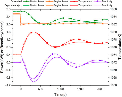
FIGURE 15. The comparison of calculated results between experimental results (Poston, 2017).
During this accident, with the decrease of engine power, heat transport power of heat pipes also reduces, leading to the increase of fuel temperature. Benefiting from the reactivity feedback of fuel, fission power gradually decreases to slow the rate of temperature rise. At about T = 300.0 s, fuel reaches the peak temperature of about 1,080.3 K. At about T = 2,200.0 s, the reactor reaches the new steady state. In the early stage of this accident, the reactor will be briefly supercritical, resulting in the increase in reactor power. This is because heat pipes absorb less power, leading to the increase of Na inventory in the reactor (Poston, 2017). The proposed model can calculate the variation of absorbed power of heat pipes. Using the feedback coefficient, this important phenomenon can be preliminarily simulated (Guo et al., 2022). This model does not directly calculate the two-phase flow of working medium in heat pipe, and the difference is acceptable.
Figure 16 shows the temperature distribution of reactor T = 0.0 s and T = 2,200.0 s respectively. Due to the high thermal conductivity of material and the compactness of this reactor, the total temperature difference of the reactor is small enough, and the peak temperature locates at the inner surface of the fuel. After the load-following accident, reactor temperature rises slightly due to the reduction of the output power of the Stirling generators. During this accident, the control rod always remains stationary, and the reactor only relies on the reactivity feedback to achieve the power regulation, showing the automatic-stability-regulation ability of this reactor.
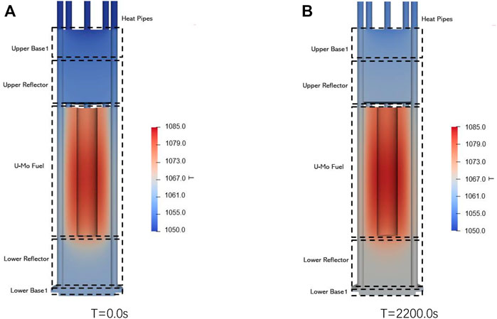
FIGURE 16. Temperature distribution of reactor. (A) T = 0.0s. (B) T = 2,200.0s.
In this paper, the super thermal conductivity model (STCM) for high-temperature heat pipe is proposed, which simplifies the vapor flow and heat transport in vapor space into heat conductance. Combined with the network method, the proposed model can preliminarily calculate the evaporation, condensation, and flow rate of working medium. Adding the heat transfer limitation, it can realize the judgment of heat pipe safety. According to the comparison with the experimental results, the accuracy of the model is verified. It can well predict the temperature variation of high-temperature heat pipes under different conditions.
Using this model, the numerical simulation on KRUSTY reactor is executed. During the steady state calculation, it can be found that the proposed model can obtain a more realistic fuel temperature distribution. For load-following transient calculation, calculated results are in good agreement with the experimental results, showing the applicability of the proposed model to this type of reactor system. It can be a powerful tool for the design and simulation of heat pipe cooled reactor systems.
The raw data supporting the conclusion of this article will be made available by the authors, without undue reservation.
YG, ZL, and ZS contributed to conception and design of the study. YG wrote the first draft of the manuscript. All authors contributed to manuscript revision, read, and approved the submitted version.
This study was funded by the National Key Research and Development Project of China, No. 2020YFB1901700, Science Challenge Project (TZ2018001), Project 11775126/11775127 by National Natural Science Foundation of China, and Tsinghua University Initiative Scientific Research Program.
The authors declare that the research was conducted in the absence of any commercial or financial relationships that could be construed as a potential conflict of interest.
All claims expressed in this article are solely those of the authors and do not necessarily represent those of their affiliated organizations, or those of the publisher, the editors and the reviewers. Any product that may be evaluated in this article, or claim that may be made by its manufacturer, is not guaranteed or endorsed by the publisher.
Annamalai, S., and Ramalingam, V. (2011). Experimental Investigation and CFD Analysis of a Air Cooled Condenser Heat Pipe. Therm. Sci. 15 (3), 759–772. doi:10.2298/tsci100331023a
Asmaie, L., Haghshenasfard, M., Mehrabani-Zeinabad, A., and Nasr Esfahany, M. (2013). Thermal Performance Analysis of Nanofluids in a Thermosyphon Heat Pipe Using CFD Modeling. Heat Mass. Transfer 49 (5), 667–678. doi:10.1007/s00231-013-1110-6
Brown, O. L. I. (1951). The Clausius-Clapeyron Equation. J. Chem. Educ. 28 (8), 428. doi:10.1021/ed028p428
Busse, C. A. (1967). “Pressure Drop in the Vapor Phase of Long Heat Pipes,” in Proc. Thermionic Conversion Specialist Conference, United States, November 1-2, 1967, 391–398.
Busse, C. A. (1973). Theory of the Ultimate Heat Transfer Limit of Cylindrical Heat Pipes. Int. J. Heat Mass Transfer 16 (1), 169–186. doi:10.1016/0017-9310(73)90260-3
Cao, Y., and Faghri, A. (1993). Simulation of the Early Startup Period of High-Temperature Heat Pipes from the Frozen State by a Rarefied Vapor Self-Diffusion Model[J]. J. Heat Transfer 114 (4), 1028–1035. doi:10.1115/1.2910655
Cao, Y., and Faghri, A. (1993). A Numerical Analysis of High-Temperature Heat Pipe Startup from the Frozen State. J. Heat Transfer 115 (1), 247–254. doi:10.1115/1.2910657
Cao, Y., and Faghri, A. (1991). Transient Two-Dimensional Compressible Analysis for High-Temperature Heat Pipes with Pulsed Heat Input. Numer. Heat Transfer, A: Appl. 18 (4), 483–502. doi:10.1080/10407789008944804
Cao, Y., and Faghri, A. (1992). Closed-form Analytical Solutions of High-Temperature Heat Pipe Startup and Frozen Startup Limitation. [J] J. Heat Transfer 114 (Nov), 1028–1035. doi:10.1115/1.2911873
Chi, S. W. (1976). Heat Pipe Theory and Practice [M]. Washington, DC: Hemispere Publishing Corporation.
Costello, F. A., Montague, A. F., and Merrigan, M. A. (1986). Detailed Transient Model of a Liquid-Metal Heat Pipe. Costello (FA), Inc NM (USA): Los Alamos National Lab
Deverall, J. E., Kemme, J. E., and Florschuetz, L. W. (1970). Sonic Limitations and Startup Problems of Heat Pipes. Los Alamos, NM (United States): Los Alamos National Lab.
El‐Genk, M. S., and Tournier, J. M. (2004). Conceptual Design of HP‐STMCs Space Reactor Power System for 110 kWe. AIP Conf. Proc. Am. Inst. Phys. 699 (1), 658–672.
Faghri, A. (2014). Heat Pipes: Review, Opportunities and Challenges. Front. Heat Pipes 5 (1). doi:10.5098/fhp.5.1
Ferrandi, C., Iorizzo, F., Mameli, M., Zinna, S., and Marengo, M. (2013). Lumped Parameter Model of Sintered Heat Pipe: Transient Numerical Analysis and Validation. Appl. Therm. Eng. 50 (1), 1280–1290. doi:10.1016/j.applthermaleng.2012.07.022
Fink, J. K., and Leibowitz, L. (1995). Thermodynamic and Transport Properties of Sodium Liquid and Vapor. Lemont, IL, United States: Argonne National Lab
Guo, Y. C., Li, Z. G., Wang, K., and Su, Z. (2022). A Transient Multiphysics Coupling Method Based on OpenFOAM for Heat Pipe Cooled Reactors[J]. Sci. China Technol. Sci. 65, 102–114. doi:10.1007/s11431-021-1874-0
Lee, C. S., Lee, D. I., and Bonilla, C. F. (1969). Calculation of the Thermodynamic and Transport Properties of Sodium, Potassium, Rubidium and Cesium Vapors to 3000°K. Nucl. Eng. Des. 10 (1), 83–114. doi:10.1016/0029-5493(69)90008-9
Levy, E. K. (1968). Theoretical Investigation of Heat Pipes Operating at Low Vapor Pressures. ASME J. Eng. Industry. 90, 547–552. doi:10.1115/1.3604687
Li, H., Jiang, X., Chen, L., Ning, Y., Pan, H., and Tengyue, M. (2015). Heat Transfer Capacity Analysis of Heat Pipe for Space Reactor[J]. At. Energ. Sci. Tech. 49 (1), 7. doi:10.7538/yzk.2015.49.01.0089
Lin, Z., Wang, S., Shirakashi, R., and Winston Zhang, L. (2013). Simulation of a Miniature Oscillating Heat Pipe in Bottom Heating Mode Using CFD with Unsteady Modeling. Int. J. Heat Mass Transfer 57 (2), 642–656. doi:10.1016/j.ijheatmasstransfer.2012.09.007
Liu, X., Zhang, R., Liang, Y., Tang, S., Wang, C., Tian, W., et al. (2020). Core thermal-hydraulic Evaluation of a Heat Pipe Cooled Nuclear Reactor. Ann. Nucl. Energ. 142, 107412. doi:10.1016/j.anucene.2020.107412
Ma, Y., Chen, E., Yu, H., Zhong, R., Deng, J., Chai, X., et al. (2020). Heat Pipe Failure Accident Analysis in Megawatt Heat Pipe Cooled Reactor. Ann. Nucl. Energ. 149, 107755. doi:10.1016/j.anucene.2020.107755
Mcclure, P. R. (2015). Design of Megawatt Power Level Heat Pipe Reactors. Los Alamos, NM (United States): Los Alamos National Lab
McClure, P. R., Poston, D. I., Clement, S. D., Restrepo, L., Miller, R., and Negrete, M. (2020). KRUSTY Experiment: Reactivity Insertion Accident Analysis. Nucl. Tech. 206 (Suppl. 1), S43–S55. doi:10.1080/00295450.2020.1722544
McClure, P. R., Poston, D. I., Gibson, M. A., Mason, L. S., and Robinson, R. C. (2020). Kilopower Project: The KRUSTY Fission Power Experiment and Potential Missions. Nucl. Tech. 206 (Suppl. 1), S1–S12. doi:10.1080/00295450.2020.1722554
Ohse, R. W. (1985). Handbook of Thermodynamic and Transport Properties of Alkali Metals. Oxford: Blackwell.
Poston, D. I. (2017). Space Nuclear Reactor Engineering. Los Alamos, NM (United States): Los Alamos National Lab
Poston, D. I. (2001). The Heatpipe-Operated Mars Exploration Reactor (HOMER). AIP Conf. Proc. Am. Inst. Phys. 552 (1), 797–804. doi:10.1063/1.1358010
Poston, D. I., Gibson, M. A., Godfroy, T., and McClure, P. R. (2020). KRUSTY Reactor Design. Nucl. Tech. 206 (Suppl. 1), S13–S30. doi:10.1080/00295450.2020.1725382
Reay, D., McGlen, R., and Kew, P. (2013). Heat Pipes: Theory, Design and Applications. Oxford, United Kingdom: Butterworth-Heinemann.
Reid, R. S. (2002). Heat Pipe Transient Response Approximation. AIP Conf. Proc. Am. Inst. Phys. 608 (1), 156–162. doi:10.1063/1.1449720
Sanchez, R., Grove, T., Hayes, D., Goda, J., McKenzie, G., Hutchinson, J., et al. (2020). Kilowatt Reactor Using Stirling TechnologY (KRUSTY) Component-Critical Experiments. Nucl. Tech. 206 (Suppl. 1), S56–S67. doi:10.1080/00295450.2020.1722553
Tien, C. L., and Chung, K. S. (1979). Entrainment Limits in Heat Pipes. Aiaa J. 17 (6), 643–646. doi:10.2514/3.61190
Tournier, J. M., and El‐Genk, M. S. (1992). ‘‘HPTAM’’heat‐pipe Transient Analysis Model: an Analysis of Water Heat Pipes. AIP Conf. Proc. Am. Inst. Phys. 246 (1), 1023–1037. doi:10.1063/1.41777
Vasiliev, L. L., and Kanonchik, L. E. (1993). Dynamics of Heat Pipe Start-Up from a Frozen State. AV Luikov Heat and Mass Transfer Institute, Byelorussian Academy of Sciences. Minsk, Belarus: CIS. unpublished data.
Wang, C., Sun, H., Tang, S., Tian, W., Qiu, S., and Su, G. (2020). Thermal-hydraulic Analysis of a New Conceptual Heat Pipe Cooled Small Nuclear Reactor System. Nucl. Eng. Tech. 52 (1), 19–26. doi:10.1016/j.net.2019.06.021
Yan, B. H., Wang, C., and Li, L. G. (2020). The Technology of Micro Heat Pipe Cooled Reactor: A Review. Ann. Nucl. Energ. 135, 106948. doi:10.1016/j.anucene.2019.106948
Yuan, Y., Shan, J., Zhang, B., Gou, J., Zhang, B., Lu, T., et al. (2016). Study on Startup Characteristics of Heat Pipe Cooled and AMTEC Conversion Space Reactor System. Prog. Nucl. Energ. 86, 18–30. doi:10.1016/j.pnucene.2015.10.002
Yue, C., Zhang, Q., Zhai, Z., and Ling, L. (2018). CFD Simulation on the Heat Transfer and Flow Characteristics of a Microchannel Separate Heat Pipe under Different Filling Ratios. Appl. Therm. Eng. 139, 25–34. doi:10.1016/j.applthermaleng.2018.01.011
Keywords: heat pipe cooled reactor, high-temperature heat pipe, STCM, heating system, KRUSTY reactor
Citation: Guo Y, Su Z, Li Z and Wang K (2022) The Super Thermal Conductivity Model for High-Temperature Heat Pipe Applied to Heat Pipe Cooled Reactor. Front. Energy Res. 10:819033. doi: 10.3389/fenrg.2022.819033
Received: 20 November 2021; Accepted: 06 January 2022;
Published: 27 January 2022.
Edited by:
Luteng Zhang, Chongqing University, ChinaReviewed by:
Chenglong Wang, Xi’an Jiaotong University, ChinaCopyright © 2022 Guo, Su, Li and Wang. This is an open-access article distributed under the terms of the Creative Commons Attribution License (CC BY). The use, distribution or reproduction in other forums is permitted, provided the original author(s) and the copyright owner(s) are credited and that the original publication in this journal is cited, in accordance with accepted academic practice. No use, distribution or reproduction is permitted which does not comply with these terms.
*Correspondence: Zeguang Li, bGl6ZWd1YW5nQG1haWwudHNpbmdodWEuZWR1LmNu
Disclaimer: All claims expressed in this article are solely those of the authors and do not necessarily represent those of their affiliated organizations, or those of the publisher, the editors and the reviewers. Any product that may be evaluated in this article or claim that may be made by its manufacturer is not guaranteed or endorsed by the publisher.
Research integrity at Frontiers
Learn more about the work of our research integrity team to safeguard the quality of each article we publish.