An Integrated AMPSO-CLSTM Model for Photovoltaic Power Generation Prediction

To address the challenges of volatile and intermittent nature in photovoltaic power (PV) generation forecasting, a new convolutional long short-term memory network (CLSTM) prediction model optimized by adaptive mutation particle swarm optimization (AMPSO) is proposed. In this model, the local sensing ability of the convolutional kernels in the CNN is used to extract high-dimensional features from the variable influential factors of PV power generation, and a mapping between time series data and PV is established by the memory ability of the gate control unit in LSTM. The AMPSO algorithm is introduced to optimize the network structure and weights of CLSTM simultaneously. The performance of the model is verified by two different two data sets. The results show that compared with that of the CLSTM, Auto-LSTM, LSTM and recurrent neural network models, the root mean square error (RMSE) of the AMPSO-CLSTM model decreases by 1.92–6.53% and 6.23–31.10%, the mean absolute error (MAE) decreases by 6.92–16.87% and 11.71–48.84%, and the mean absolute percentage error (MAPE) decreases by 13.24–31.75% and 12.22–49.00%, respectively. Compared with those of the CLSTM model, the number of channels in the convolutional layer of the AMPSO-CLSTM is reduced by 51.76–71.09% and 61.72–86.72%, respectively, and the number of hidden neurons in LSTM is reduced by 32–60% and 53–84%, respectively.

Introduction

Solar PV power generation uses the PV effect to convert solar radiation into electricity. PV power utilization limits fossil fuel usage and reduces carbon dioxide, sulfur oxide and nitrogen oxide emissions. Global PV power generation has great potential, and vigorously developing solar PV power generation is an important way to protect the global environment and respond to climate change. After the signing of The Paris Agreement (Unfccc, 2015), global PV power generation has grown rapidly. The cumulative installed capacity increased from 217,463 MW in 2015 to 707,495 MW in 2020, and the annual power generation increased from 242 TWh in 2015 to 693 TWh in 2019 (IRENA, 2021), becoming an important primary energy resource able to replace fossil fuel energy. The intensity of the PV effect depends strongly on solar irradiance. Solar irradiance is related to complex meteorological factors; thus, the output power of PV power generation systems is easily affected by meteorological factors and has strong volatility and randomness (Abdel-Nasser and Mahmoud, 2019). This characteristic increases the risk to power supply dispatching and power system operation, resulting in increased cost. Therefore, accurate PV power forecasting can not only enable the development of a peak regulation plan for PV power in advance, result in reasonable power supply scheduling, and improve the operational safety of a power system but also improve the capacity of PV power generation in an electric grid, reduce economic losses caused by power rationing and increase the return on investment of PV power stations. In addition, accurate PV power prediction can provide decision support for the operation of PV power stations, such as the arrangement of equipment overhaul and maintenance under long-term durations without light or under low light. Therefore, the use of a new prediction model to forecast the output power of PV power generation systems is very important.

Over the past few decades, many scholars have conducted research on wind power and PV power generation prediction. Early studies were based mainly on statistical models, such as the autoregressive integrated moving average (Jing et al., 2011), multiple linear regression (Trigo-González et al., 2019), and fuzzy theory (Shaker et al., 2020). The statistical model is more sensitive to the time range and quality of the input data and can produce more accurate short-term PV power prediction results (Li et al., 2020). However, statistical models are generally used only for a small amount of data and a small number of influential factors, and their prediction performance on large sample data is not ideal.

With the continuous improvement in computer performance, prediction model ANNs based on machine learning are being used more widely in PV power generation prediction. A neural network prediction model mimics the structure of the dendrites and axons of biological neurons, as well as neural activation and inhibition. These models can realize human perception, learning, memory, recognition and other behaviors (Mcculloch and Pitts, 1943) and have a good effect on complex mapping modeling and system identification (Narendra and Parthasarathy, 1989). In addition, the BP algorithm (Rumelhart et al., 1986) is introduced to enhance the learning and fitting ability of neural network models. Therefore, ANNs have been widely used in PV power generation prediction. For example, Al-Dahidi et al. (2019) proposed an efficient ANN to analyze the relationship between the total solar radiation and climate variables and predicted the solar radiation of the Shafa Badran Amman, Jordan. Chu et al. (2015) developed an artificial neural network to predict the real-time output of PV power stations. Similar ANN prediction models can be found in studies of Zhang et al. (2020) and Khandakar et al. (2019). Compared with ANN, Buwei et al. (2018) proposed a SVM model based on data fusion, and the model obtains a more accurate data set in prediction. In addition, Zhou et al. (2020) used ELM to predict PV power generation.

These traditional shallow machine learning models have difficulty learning the deep nonlinear relationship between the variable meteorological conditions and PV power generation. Therefore, a neural network model based on deep learning is proposed and applied to the PV power generation prediction problem. Deep learning models are a new research direction in the field of machine learning. By deepening the network level, the high-dimensional features are gradually extracted from the low-level features. A series of methods (such as dropout and regularization) are used to counter the overfitting caused by the deep level. Deep learning models include CNNs, DBN, stacked autoencoders, RNNs, GAN and other classical models, as well as their variants and numerous combinations. Compared with the shallow ANN, the deep learning model has a stronger fitting ability and is better at discovering complex structures in high-dimensional data (Lecun et al., 2015). At the same time, deep learning can be used to automatically identify the input features and discover the relations between features, which reduce the necessity of feature engineering for data. For example, Ghimire et al. (2019b) used DBN and DNN to predict long-term global solar radiation. Compared with other 15 feature selection methods, the absolute percentage bias and high Kling-Gupta efficiency values of the deep learning model were significantly reduced. Zhang et al. (2022) proposed a geological prediction model based GAN (GAN-GP). The generator of the model includes feature extraction and integration modules, which are, respectively, used to extract important features from operation data and generate geological condition prediction. The experimental results show that the model is effective in geological prediction.

As a typical deep learning neural network model, the LSTM network is very popular in the field of prediction due to its long-term memory and ability to process time series. For example, Zhang et al. (2018) built a prediction model for LSTM PV power generation. An experiment showed that its performance was better than that of MLP and the deep convolutional network. Qing and Niu (2018) used a LSTM network to predict hourly and day ahead solar irradiance and insisted that the results are than BP and linear least square regression. Similar studies conclusions on LSTM better performance can be found in Han et al.’s (2019) and Luo et al.’s (2021) studies. Compared with the shallow ANN, LSTM offers a certain improvement in prediction performance, but on high-dimensional data, the processing ability is not strong. To improve its performance, studies often enhance the time correlation of the prediction model by increasing the input dimensions (Nargesian et al., 2017). However, with the increase in the input dimensions and number of layers of the LSTM network, the complexity of the LSTM structure and the excessive matrix computation have seriously affected the training speed of the prediction model (Chai et al., 2019).

One solution is combine CNNs, RNNs, ESNs and other models into hybrid deep learning models, which can make full use of the advantages of the various algorithms to improve the prediction performance. In the field of PV prediction, for example, Iversen et al. (2017) and López et al. (2018) proposed a prediction model combining LSTM and an ESN and applied it to predict the wind power of the Klim Fjordholme power plant in Denmark. (Wang et al., 2019b). proposed a hybrid LSTM-convolutional network for photovoltaic power prediction and showed that hybrid prediction model has better prediction effect than the single prediction model. Ghimire et al. (2019a) combined the pattern recognition ability of CNN and the time series processing ability of LSTM to predict global solar radiation and showed that the prediction results of the proposed hybrid model are better than those of the benchmark model. Besides, Auto-LSTM model, an autoencoder is added to the LSTM model as the data feature extractor (Alkandari and Ahmad, 2020) and the performance of the proposed Auto-LSTM model was verified on the Shagaya Renewable Energy Park data set in Kuwait (Marion et al., 2014). Similar hybrid deep learning models in PV power generation were developed by Yona et al. (2013), Bouzerdoum et al. (2013), and Zang et al. (2020).

Among these mixed models, the CLSTM model combines the ability of the CNN to extract high-dimensional features and the ability of LSTM to process time series data; thus, it is more suitable for PV power generation prediction. Compared with the CNN and LSTM, CLSTM has higher prediction accuracy, stability and robustness (Wang et al., 2019a). However, in the CLSTM model, the selection of network structure parameters is usually carried out through a trial-and-error method. This experience-based method is time consuming, laborious and subjective, and the obtained hyperparameters are not optimal, leading to limited model performance (Bergstra and Bengio, 2012). Therefore, determining the network structure effectively is an important problem to be solved in this kind of research.

An important way to carry out neural network structure determination is to introduce intelligent algorithms, such as PSO, GA and the ant colony algorithm. For example, Vaitheeswaran and Ventrapragada (2019) used the GA to optimize the time window size of LSTM and tested the optimized LSTM-based prediction model on the data of the 2012 Global Energy Forecast Competition. Shahid et al. (2021) optimized window size and number of neurons in LSTM layers by GA and improved wind power predictions from 6 to 30% as opposed to existing techniques. Considering the nonlinear and stochastic behavior of grid users, Hafeez et al. (2020) proposed a load forecasting model based on factored conditional restricted Boltzmann machine. Mamun et al. (2019) used the GA to optimize the time window, number of neurons and batch size of the LSTM model to construct a hybrid power load prediction algorithm. Neshat et al. (2021) proposed a new evolutionary model based on deep learning for wind speed prediction. The improved generalized normal distribution optimization algorithm is used to optimize the hyper-parameters of bidirectional LSTM. These studies have made much progress in improving the network prediction effect and network performance. However, for PV forecast research, the following research gaps still need to be studied:

First, in the modeling of PV power generation, data are classified by day and other methods (Nam et al., 2020), and different models are built for different types of data (such as different seasons). This approach may break the entire data set into many smaller data sets (different seasons, different regions, etc.). In the case of insufficient data, the decomposed sub-data set may be very small: thus, the model easily overfits during training. Therefore, to ensure that all categories of data have a good prediction effect, a sufficient data volume is needed to support the usage of these methods.

Second, instead of optimizing the structure and weight of the deep learning network at the same time, the existing network optimization using PSO or the GA usually optimizes only the network structure (Huang et al., 2020) or the weights of the network (Bashir and El-Hawary, 2009). When optimizing the structure, the traditional BP algorithm, which easily falls into the local optimum, is still used to train the weight (Chan and Fallside, 1987). When optimizing the weight, the network structure is still determined by the trial-and-error method. On the one hand, much time is required to try each parameter combination. This method’s retrieval process in the search space involves jumping and is discontinuous, and high-performance solutions could appear in the skipped search spaces (Kim and Cho, 2019). On the other hand, manual determination depends on the operator’s own experience and thus is a very subjective method. Therefore, how to optimize the network structure and weight parameters simultaneously requires further research.

Therefore, to compensate for the disadvantages of finding the optimal structure and weights of the CLSTM prediction model, this paper proposes a CLSTM prediction model optimized by adaptive mutation particle swarm optimization (Tang and Zhao, 2009), named AMPSO-CLSTM. The model uses the real-time monitoring meteorological data of PV power stations as input and uses the AMPSO algorithm to optimize the CLSTM network structure and weights simultaneously to obtain the best structure-weight combination. On the one hand, the binary encoding part and real encoding part of particles in AMPSO, corresponding to the structure and weights of the network are optimized. It can determine the optimal network structure effectively without manually adjusting parameters or using grid search to find the optimal network structure. On the other hand, the combination of AMPSO global optimization and the BP local fast algorithm can improve network learnability and help the model jump out of local optimality. The operation data of two power stations are used to verify the model’s prediction performance. The results show that compared with other models, the RMSE, MAE and MAPE of AMPSO-CLSTM model on the two data sets have decreased in varying degrees.

The paper is organized as follows: Introduction describes previous related studies about PV prediction. Section 2 introduces the AMPSO-CLSTM model used for power prediction in this study. Experiments on Photovoltaic Power Prediction shows the performance of the proposed model using the data of two regions. Conclusion draws conclusions.

Methodology

A Brief Introduction to CLSTM

LSTM is a kind of improved RNN. It overcomes the disadvantages of long-term dependence on the RNN and gradient vanishing by adding structures such as “gate units” and “cell states” (Greff et al., 2017). Various gates of LSTM not only provide the ability to retain long-term dependency but also can carry out the nonlinear mapping of complex data to establish long-term memory in the time dimension; thus, LSTM has a strong advantage in the preservation and learning of temporal sequence information. However, its ability to extract high-dimensional features is poor. Therefore, CNN feature extraction has been introduced in some studies to compensate for the deficiency of LSTM (Wang et al., 2019a).

A CNN is a kind of neural network with a special linkage mode. In the convolutional layer, a linear operation named a convolution is adopted to replace the fully connected mode in the traditional neural network. In addition to the convolutional layer, a CNN also contains structures such as an activation layer, a pooling layer and a fully connected layer. Through nonlinear convolution on complex data, the network extracts high-dimensional feature graphs. CNN can extract local features of data from high-level input and transfer them to low layer to make the network obtain more complex features. It is assumed that layer $l$ is the convolution layer. Its operation mode is shown in Eq. 1:

$z_g^l=\sigma \left(b_g^l+{\displaystyle \sum _{r=1}^R{w}_{rg}^l\otimes z_r^{l-1}}\right)(1)$

Where $w_{rg}^l$ and $b_g^l$ are the weight and bias of the $r$ ^th convolution operation of the $g$ ^th convolution kernel of layer $l$, respectively. When $l=1$, $z_g^0$ is the input vector of PV power prediction such as temperature and radiation.

A CNN is introduced into LSTM to extract the features of input data, forming a hybrid model, CLSTM. This network uses the convolutional layer to simulate the response actions of individual neurons to stimuli. The CNN applies the convolutional operation to the original time series data to extract the spatial features of multiple time series data sets and transfers the denoised features to the LSTM layer below. As the next layer of the CNN, the LSTM layer is used to capture the time series pattern of data. Taking a 1D-CNN and multi-input-single-output LSTM as examples, the constructed CLSTM structure is as shown in Figure 1.

FIGURE 1

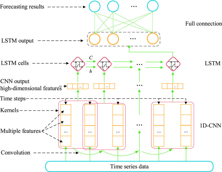
FIGURE 1. Structure of the CLSTM prediction model.

Compared with the traditional LSTM network, the CLSTM hybrid model uses a CNN to preprocess the data; thus, it has a stronger feature extraction capability. That is, the model can find the relationship among the multifactor input data and build a mapping between the input and output. The hybrid model overcomes the disadvantages of the CNN in dealing with time series and the difficulty faced by LSTM in feature extraction. At the same time, compared with feature extraction using a fully connected layer, the use of the CNN can decrease the number of parameters to be trained by the network, reduce the model complexity and prevent overfitting to a certain extent, thus enabling the construction of a deeper network structure (Xiong et al., 2020).

Adaptive Mutation Particle Swarm Optimization

AMPSO is an improved version of traditional PSO algorithm. The algorithm aims to improve the global search capability of PSO and avoid falling into local optima (Alfi, 2011). AMPSO turns the static inertia weights and learning factors of the traditional PSO into adaptive dynamic parameters. In AMPSO, the update equations of particle velocity and position are shown in Eqs 2 and 3 (Tang and Zhao, 2009):

$v_m\left(t+1\right)={\omega }_m{v}_m\left(t\right)+c_1{r}_1\left(pbes{t}_m-x_m\right)+c_2{r}_2\left(gbest-x_m\right)(2)$

$x_m\left(t+1\right)=x_m+v_m\left(t+1\right)(3)$

Eq. 3 indicates that the velocity $v_m\left(t+1\right)$ of the particle $m$ at the next moment is determined by the current velocity $v_m\left(t\right)$. Eq. 4 indicates that the position $x_m\left(t+1\right)$ of the particle $m$ at the next moment is determined by the current position $x_m\left(t\right)$ and the velocity at the next moment $v_m\left(t+1\right)$.

In Eq. 3, $r_1$ and $r_2$ are random numbers, belongs to $\left[\mathrm{0,1}\right]$. ${\omega }_m$ is adjusted according to $fit\left(P_m\right)$, and the average fitness ($fi{t}_{ave}$) and the maximum fitness ($fi{t}_{\max }$) of all particles, as shown in.

${\omega }_m=\frac{\eta \times \left(fit\left(P_m\right)-fi{t}_{\max }\right)}{fi{t}_{ave}-fi{t}_{\max }}(4)$

Where $\eta$ is a random number between [0, 1]. The results show that when the particles are dispersed (the value of $fi{t}_{ave}-fi{t}_{\max }$ is large), ${\omega }_m$ is adjusted to a smaller value to ensure that the particles can quickly approach the optimal position of the particle swarm. On the contrary, the inertia weight increases to help the particles jump out of the local optimum.

The learning factors $c_1$ and $c_2$ control the effects of their own optimal position ($pbes{t}_m$) and population optimal position ($gbest$) on particle motion, respectively. In traditional PSO, $c_1=c_2=2$. However, in different stages of particle optimization, the proportion of learning from self-optimum and population optimum should not be constant. When it is far from the global optimization, the particle should first approach the population optimization to accelerate the convergence of the model while the particle is very close to the global optimum, the particle optimization speed decreases (Alfi, 2011). In this scenario, particles need more reference to their own optimal, to jump out of the local optimal situation and to find a better solution. Adaptive learning factor is introduced into AMPSO as Eqs 5 and 6:

$c_1=c_{1s}+\frac{gen}{max\_gen}\times \left(c_{1e}-c_{1s}\right)(5)$

$c_2=c_{2s}+\frac{gen}{max\_gen}\times \left(c_{2e}-c_{2s}\right)(6)$

Where $c_{1s},c_{2s}$ and $c_{1\text{e}},c_{2e}$ are, respectively, the initial and final values of learning factors $c_1$ and $c_2$. With the increase of interation, the value of $c_1$ increases linearly in the range of initial value and final value, while $c_2$ decreases linearly. In the early stage of convergence, the particle swarm is much affected by $c_2$, and can get closer to the optimal population faster. However, in the later stage of convergence, the particle is easy to fall into the local optimum, and $c_1$ has a greater impact on the particle velocity, and the particle tends to move to its own optimal position, so it is easier to jump out of the local optimum.

Moreover, AMPSO introduces the uniform mutation operation of GA (Wang et al., 2013) to improve the richness of particle $m$ position through random disturbance as .

$x{\mathrm{\prime }}_{mi}=a_1+\delta \left(a_2-a_1\right)(7)$

Where, $\delta$ is a random number between [0 and 1], $x_{mi}^{\text{'}}$ is a random number that obeys uniform distribution in the particle search space $\left[a_1,a_2\right]$, and represents the mutated value of the $i$ component of particle $m$. $x_{mi}$ is replaced by $x_{mi}^{\text{'}}$ to update the position of particle swarm. By randomly selecting particles for mutation operation, the forward direction of particles can be changed and particles can enter other regions for search. In the subsequent search process, the algorithm may find new $pbest$ and $gbest$.

AMPSO-CLSTM Prediction Model

Framework

To obtain the structures in the CLSTM deep prediction model, such as the number of convolutional layers, the size of the convolutional kernel, the number of network hidden units and the weights of the neuronal connections, this paper introduces the AMPSO algorithm to optimize the structure and weights simultaneously. Compared with the independent design scheme of structure optimization and network training in previous studies, this paper adopts mixed coding in AMPSO, which includes both binary encoding and real encoding, to synergistically optimize the network structure and weight. Binary encoding corresponds to the structure of CLSTM. If the encoding value is 1, the corresponding neuron is enabled. A code value of 0 indicates that the neuron is not enabled. The real code corresponds to the CLSTM weights, and each bit of code corresponds to the value of a weight in the network. The AMPSO algorithm optimizes the binary coding part that determines the network structure by updating the coding values of different locations from 0 to 1 (or from 1 to 0) to produce different combinations of neurons to obtain the optimal network structure in evolution. Under a certain network structure, the real coded particle is combined with the BP algorithm to obtain the optimal network weights. The network framework is shown in Figure 2.

FIGURE 2

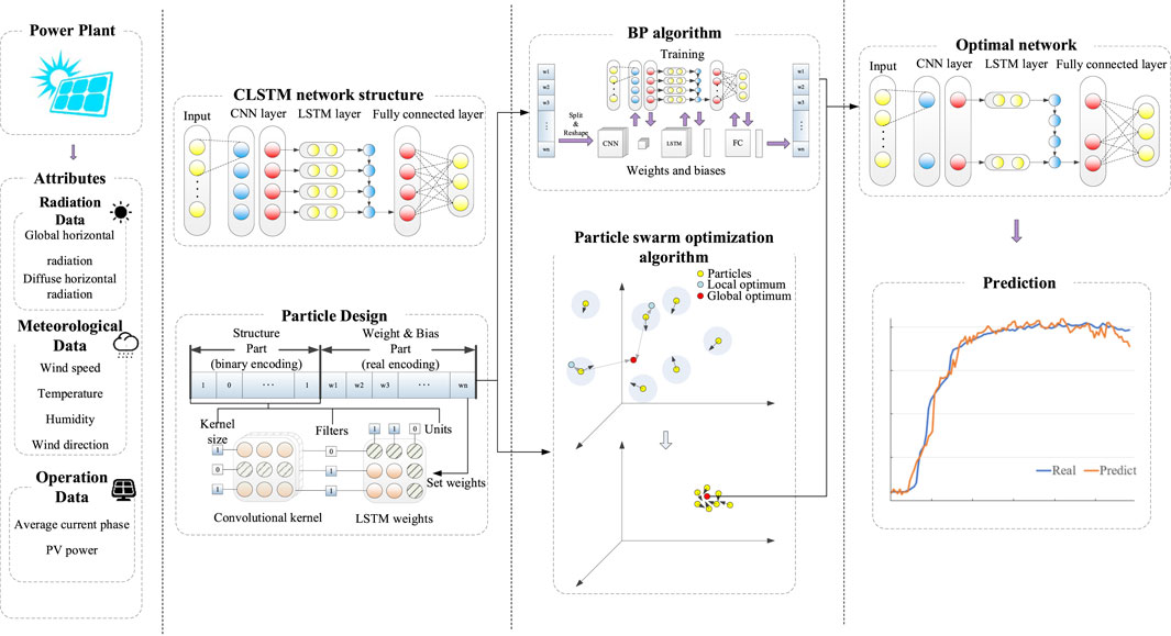
FIGURE 2. Framework of the AMPSO-CLSTM prediction model.

Prediction Processes of the AMPSO-CLSTM Model

The AMPSO-CLSTM model proposed in this paper is a hybrid model combining CLSTM with a 1D-CNN and the multi-input-single-output mode. The CNN is used to extract the high-dimensional features of meteorological data and connect with the LSTM layer to establish a mapping between the meteorological data and PV output power. AMPSO is used to optimize the structural parameters, such as the numbers of channels and hidden layer units, and the weights of CLSTM. The process is shown in Figure 3.

FIGURE 3

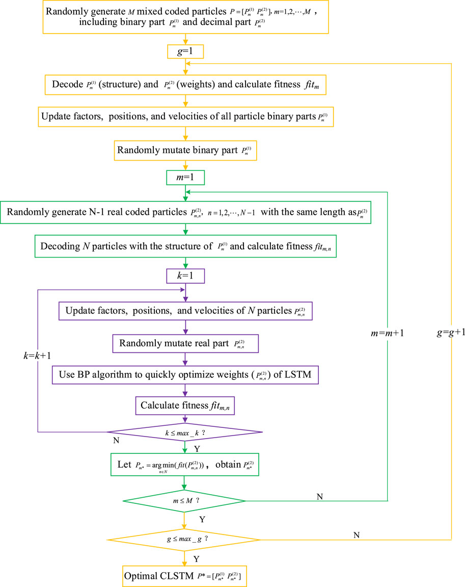
FIGURE 3. Flowchart of AMPSO-CLSTM.

The details of the optimization processes in the proposed AMPSO-CLSTM model are as follows.

Step 1. Initialize the inertia factor, learning factors, mutation chance, max velocity of the particles ($v_{\max }$), and max iteration of the optimization in the binary part ($\max \_gen$) and real part ($\max \_k$). Randomly generate $M$ mixed coded particles $P_m=\left[P_m^{\left(1\right)},P_m^{\left(2\right)}\right],m=\mathrm{1,2},\mathrm{...},M$, including the binary part $P_m^{\left(1\right)}$, which contains the network structure, and decimal part $P_m^{\left(2\right)}$, which contains the network weights and biases.

Step 2. gen = 1.

Step 3. Decode $P_m^{\left(1\right)}$ and $P_m^{\left(2\right)}$, and then calculate the fitness $fit\left(P_m\right)$ with Eq. 8:

$fit\left(P_m\right)=\sqrt{\left({{\displaystyle \sum _{j=1}^n\left[y\left(j\right)-\overline{y}\left(j\right)\right]}}^2\right)/n-1}(8)$

where $y\left(j\right)$ is the label of sample $j$ and $\overline{y}\left(j\right)$ is the output of the network decoded from $P_m$ when using sample $j$ as the input.

Step 4. Update the inertia factor and learning factors of $P_m^{\left(1\right)}$ with Eqs 4–6. Update the velocity of the particle with Eq. 2. Update the positions of all particle binary parts $P_m^{\left(1\right)}$ with Eqs 9 and 10 and the positions of all particle decimal parts $P_m^{\left(2\right)}$ with Eq. 11.

$s\left(v_i\right)=\frac{1}{1+\exp \left(-v_i\right)}(9)$

$x_i=\{\begin{array}{l}{x}_{i}if\text{ rand}\left(\right)<s\left(v_i\right)\\ 1-x_{i}otherwise\end{array}(10)$

$x_i\left(t+1\right)=x_i\left(t\right)+v_i\left(t+1\right)(11)$

Here, $v_i$ is the velocity of the $i$ component of the particle, and $s$ is the probability of changing the position of a particle.

Step 5. Randomly mutate the binary part $P_m^{\left(1\right)}$; that is, a certain probability exists for the binary part $P_m^{\left(1\right)}$ to change from 0 to 1 or from 1 to 0.

Step 6. Let $m=1$.

Step 7. Randomly generate N-1 real coded particles $P_m^{\left(2\right)},n=\mathrm{1,2},\mathrm{...},N-1$, that have the same length as $P_m^{\left(2\right)}$. Let $P_{m,N}^{\left(2\right)}=P_m^{\left(2\right)}$.

Step 8. Decode $P_{m,n}^{\left(2\right)}$ with the structure of $P_m^{\left(1\right)}$, and calculate the fitness $fit\left(P_{m,n}^{\left(2\right)}\right)$ with Eq. 8.

Step 9. $k=1$.

Step 10. Update the inertia factor and learning factors of $P_{m,n}^{\left(2\right)}$ with Eqs 4–6. Update the velocity and position of $P_{m,n}^{\left(2\right)}$ with Eqs 2 and 3.

Step 11. According to Eq. 7, the mutation operation is performed on the new particle $P_{m,n}^{\left(2\right)}$, taking $a_1=-1$, $a_2=1$, that is, some positions of the new particle $P_{m,n}^{\left(2\right)}$ have a certain probability to be replaced by random numbers uniformly distributed on $\left[-\mathrm{1,1}\right]$.

Step 12. Optimize the weights and biases [$P_{m,n}^{\left(2\right)}$] of CLSTM by BP. Decode $P_{m,n}^{\left(2\right)}$ with the structure of $P_m^{\left(1\right)}$, and calculate the fitness $fit\left(P_{m,n}^{\left(2\right)}\right)$ with Eq. 1.

Step 13. $k=k+1$. If $k\le \max \_k$, go to Step 14; otherwise, go to Step 10.

Step 14. Let $P_{m\ast }=\underset{n\in N}{\arg \min }\left(fit\left(P_{m,n}^{\left(2\right)}\right)\right)$, and obtain $P_{m\ast }^{\left(2\right)}$.

Step 15. $m=m+1$. If $m\le M$, go to Step 16; otherwise, go to Step 7.

Step 16. $gen=gen+1$. If $gen\le \max \_gen$, go to Step 3; otherwise, obtain the optimal CLSTM structure and weight combination $P^{\ast }=\left[P_{m\ast }^{\left(1\right)},P_{m\ast }^{\left(2\right)}\right]$.

Experiments on Photovoltaic Power Prediction

Parameter Settings

To evaluate the performance, the proposed AMPSO-LSTM was verified using the data of the 1B site of the DKASC PV system in Alice Springs, Australia (DKASC, 2020), and the data of the Wuzhong Taiyangshan PV power station in Ningxia, China (Taiyangshan, 2016).

Missing and abnormal values are noted for the data recorded at the power stations. If these missing and abnormal values are not well treated, the model fitting results will be biased, thus misleading users in their decision making. Therefore, the missing and abnormal values need to be cleaned before data are input into the model. In this study, the abnormal values were regarded as missing values and were interpolated by cubic spline interpolation. Cubic spline interpolation is a smooth curve passing through a series of shape value points. The interpolation method has good convergence and stability. The definition of cubic spline function is: let there be interpolated nodes $d_1={\alpha }_1<{\alpha }_2<\cdots <{\alpha }_n=d_2$ on $\left[d_1,d_2\right]$ corresponding to the function values of $y_1,y_2\cdots y_n$. If $\Phi \left(\alpha \right)$ satisfies $\Phi \left({\alpha }_j\right)=y_j\left(j=\mathrm{1,2},\cdots ,n\right)$, $\Phi \left(\alpha \right)$ is not a polynomial higher than cubic on $\left[{\alpha }_j,{\alpha }_{j+1}\right]\left(j=\mathrm{1,2},\cdots ,n-1\right)$, and when $\Phi \left(\alpha \right)$ has second-order continuous derivative on $\left[d_1,d_2\right]$, $\Phi \left(\alpha \right)$ is called cubic spline function (Xu and Zhong, 2006). To uniquely determine a cubic spline interpolation function, two boundary conditions are needed. In this paper, the Not-A-Knot Spline is used to determine the missing and abnormal values in the experiment. For example, in the experimental data of case 1, the data of 21:10 on 5 January 2014 is the missing value. The cubic spline interpolation method is used to preprocess the data. The output power of PV power generation on 5 January 2014 before and after processing is shown in Figure 4. After data cleaning, standardization was applied to process different influential factors into similar data dimensions.

FIGURE 4

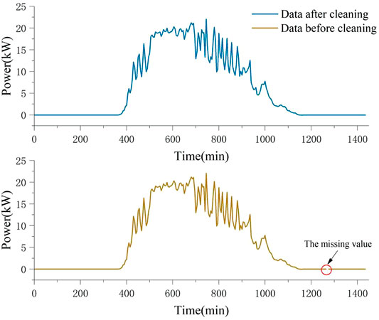
FIGURE 4. The data before and after cleaning.

Weight initialization is a very important step in the deep learning algorithm. Reasonable initial weights can help the algorithm converge faster and avoid gradient vanishing and gradient explosion. To ensure the fairness of the comparison between different algorithms, the same initialization method was adopted for the weights of different algorithms. In this paper, Xavier initialization (Glorot and Bengio, 2010) was adopted to generate the initial weights; the distribution of its initialization is shown in Eq. 12:

$w\sim U\left[-\frac{\sqrt{6}}{\sqrt{fa{n}_{in}+fa{n}_{out}}},\frac{\sqrt{6}}{\sqrt{fa{n}_{in}+fa{n}_{out}}}\right](12)$

where $fa{n}_{in}$ and $fa{n}_{out}$ represent the number of input nodes and the number of output nodes of this layer, respectively. The transmission of data with appropriate diversity in each layer can be done to effectively carry out neural network learning. If the variance of each input layer cannot be kept within a stable range, the gradient may disappear and explode in the training process. Xavier initialization can generate evenly distributed initial weights so that all layers are evenly activated, which effectively solves the above problems and is conducive to neural network learning.

Model Performance Comparison

In this section, the results of the proposed model are analyzed and compared with those of other models. This model’s computational complexity is $\left(S\times P\times F+F\times U+U^2\right)\times M$. A personal computer with a CPU i7-9750 h is used for calculation. Under these conditions, the average training time of AMPSO-CLSTM is 435.1 $\mu s$ per step and 4 $s$ per epoch.” This study is based on Python 3.5 and TensorFlow 1.4.0 (a machine learning platform with high flexibility and excellent computing performance).

DKASC PV System

The experiment uses real data from the 1B DKASC PV System in Alice Springs, Australia. The site 1B consists of four trackers. The technical specifications of this power system are shown in Table 1.

TABLE 1

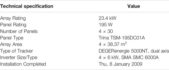
TABLE 1. Technical specifications of the DKASC power system.

The sensors of the power system record radiation data (such as the total radiation and direct radiation at water level), meteorological data (such as wind speed, temperature, relative humidity and wind direction), and system operation data (such as the average current phase and active power). Considering that few factors affect the PV power generation of power stations and that wind direction data should not be directly input into the model, a data augmentation method is adopted to expand the data. The sine value and cosine value of the wind direction angle are used as part of the network input instead of the wind direction angle data. Before the start of the experiment, the data sets should be partitioned: the data from 1 January 2014, to 31 December 2015, are selected for this experiment, and the data resolution is 5 min. The data from 2014 are used for training the network, and the data from 2015 are used as the test set.

Table 2 shows the details of the hyperparameters of the model used in the experiment, among which the hyperparameters of LSTM and CLSTM are from (Wang et al., 2019a) and the hyperparameters of the RNN and Auto-LSTM are obtained by trial and error. The hyperparameter maximum setting of AMPSO-CLSTM is consistent with the hyperparameter setting of CLSTM to ensure that its solution space contains the values of the CLSTM hyperparameters. In addition, the maximum iterations $\max \_gen$ and $\max \_k$ are set according to the calculation complexity of the algorithm and the evolutionary iterations when the results tend to be stable in the preliminary trial calculation.

TABLE 2

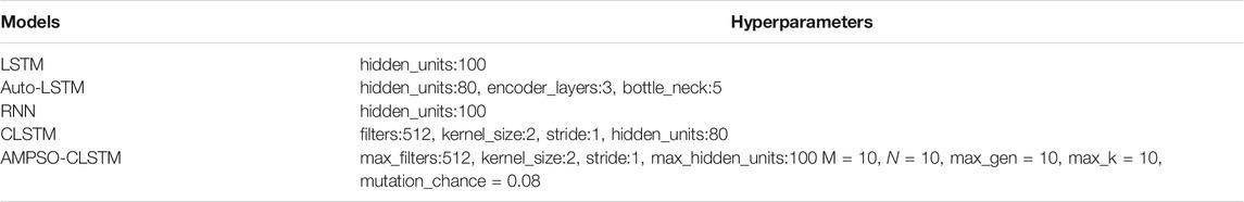
TABLE 2. Hyperparameter settings in the proposed model.

To compare the model proposed in this paper with the algorithms used in previous studies, some indicators need to be used to measure the performance of different algorithms. The selected performance indicators are: MAE, RMSE, and MAPE. The calculation methods of the three performance indicators are as follows:

$MAE=\left({\displaystyle \sum _{j=1}^n|y\left(j\right)-\overline{y}\left(j\right)|}\right)/n(13)$

$RMSE=\sqrt{\left({{\displaystyle \sum _{i=1}^n\left[y\left(j\right)-\overline{y}\left(j\right)\right]}}^2\right)/n-1}(14)$

$MAPE=\left({\displaystyle \sum _{j=1}^n|\left[y\left(j\right)-\overline{y}\left(j\right)\right]/\left(j\right)|}\right)/n(15)$

where $y\left(j\right)$ is the sample label of data $j$, $\overline{y}\left(j\right)$ is the output value obtained by inputting data $j$ into the network, and $n$ is the number of data.

To measure and compare the robustness of the models, we perform 50 independent calculations on each model. The boxplots of the RMSE, MAE and MAPE indexes of all models for the 50 independent operations are shown in Figure 5.

FIGURE 5

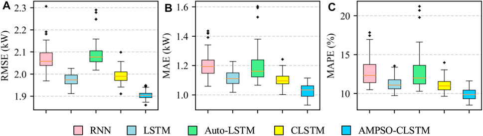
FIGURE 5. Boxplots of error indexes for 50 independent runs on the DKASC data set. (A-C) are the RMSE, MAE and MAPE of all models, respectively.

From Figure 5, among the three error indicators, the proposed AMPSO-CLSTM model has the smallest mean value and a small fluctuation range. The accuracy of the LSTM model is similar to that of CLSTM in terms of the MAE and MAPE indexes, and LSTM has a lower RMSE than that of CLSTM. This result is similar to that obtained by Wang et al. (2019a). The author believes that when the data length is only 1 year, the time feature in the data is relatively strong and the spatial feature is weak; thus, CLSTM cannot extract the spatial feature of the data easily. Compared with the RNN, the LSTM and CLSTM models have more accurate prediction results and lower volatility, which shows that the special LSTM gate unit has a certain robustness against gradient vanishing and gradient explosion. The prediction accuracy and volatility of the Auto-LSTM model are not satisfactory, which may be caused by the small input dimensions of the data set. When the input dimensions are small, they do not need to be reduced, and the use of an autoencoder for data processing may lead to information loss.

The proposed model is compared with the RNN, LSTM, CLSTM and Auto-LSTM models, and the results with the minimum RMSE over 50 independent runs of each model are selected. Three error evaluation indexes, i.e., RMSE, MAE and MAPE, are used to measure the model performance to further verify the improvement effect of the proposed model on the prediction accuracy. Table 3 shows the RMSE, MAE and MAPE indexes of the different models for summer (December to February), autumn (March to May), winter (June to August), spring (September to November) and the whole year. The AMPSO-CLSTM model proposed in this paper clearly performs well in predicting PV power in different seasons. On the MAE and MAPE indexes, the proposed model has the best performance. On the RMSE index, the performance of this model is slightly lower than that of the CLSTM model in spring (0.85%), but the forecasting effect for the other seasons and the annual averages are the best. The proposed model is clearly good compared with the RNN, LSTM, CLSTM and Auto-LSTM models in predicting PV output power 1 hour in advance.

TABLE 3

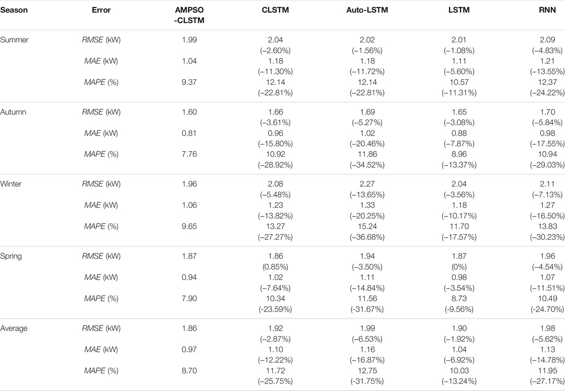
TABLE 3. PV power forecasting error for each season.

To further analyze the fitting effect for different seasons, 4 days are randomly selected from each season to draw the forecast results of the proposed model and the comparison model, as shown in Figure 6. All the models have good prediction results under gentle meteorological conditions from 5:00 to 19:00, but the proposed model has a steady and more accurate prediction curve, and its prediction results are closer to the actual value. When the meteorological conditions change dramatically and rapidly (such as in summer and winter), the PV output power prediction accuracy of all the models decreases slightly, but the prediction results of the proposed model remain stable despite the variation in PV output power. During data collection at the power stations, noise or incorrect data may be generated due to errors or faults in the sensors themselves. Although we filled in the missing values and abnormal values in the data before training, no method exists for preprocessing this noise data with high-frequency fluctuations within a reasonable range. If the model perfectly fits the highly volatile data with high-frequency noise, then it has overfitted the data, which will affect the accuracy of the PV output power prediction by the model in the future. The proposed model can be stabilized around the trend of the curve in the case of high-frequency fluctuation of the output data, which indicates that the model has the ability to deal with noise.

FIGURE 6

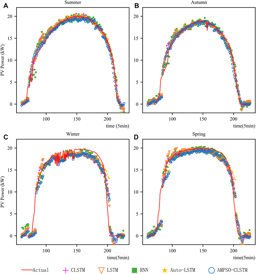
FIGURE 6. Forecasting results for a whole day in each season. (A-D) respectively show the forecast results of all the models in spring, summer, autumn and winter.

To verify the prediction accuracy of the model under different weather conditions, a sunny day and a rainy day were randomly selected from the test set, and the prediction results, prediction errors, and regression analyses were plotted, as shown in Figure 7. Figures 7A,D plot the observed PV power output from 5:00 to 19:00 on the selected sunny and rainy days, respectively, as well as the predicted values for each model, and Figures 7B,E plot the percentage errors of the predicted values and the observed values for this time period. Figures 7C,F plot the regression analyses for the sunny and rainy days with the observed PV power output as the horizontal coordinate and the predicted value of each model as the vertical coordinate and calculate the R² values of each model. Figures 7A,D show that all models can fit the PV output power curve well under sunny conditions, but the AMPSO-CLSTM model proposed in this paper has less volatility and a higher prediction accuracy. On cloudy and rainy days, the error of the selected model is slightly larger than that on sunny days because the light conditions and humidity on the rainy days changed rapidly, which was difficult for the model to fit. However, all models are still able to capture the trend of the PV output power, with the fluctuation range of the CLSTM and the proposed AMPSO-CLSTM model being smaller. Hence, the combined network architecture of the CNN and LSTM can improve the fitting ability of the network to a certain extent. The percentage errors shown in Figures 7B,E show that the prediction error of the model in the early morning and evening is larger. In the morning and afternoon, the prediction accuracy of the model is higher, with the error typically remaining below 10%, because the solar irradiance, which has a significant impact on the PV output power, changes rapidly in the early morning and evening and the models have difficulties fitting the curve. Figures 7C,F show that the models made predictions with high accuracy for PV output power observations above 12 kW. When the power output is below 12 kW, fluctuations occur because the time period during which the observed value of the PV output power is less than 12 kW is mainly concentrated in the early morning and evening, when the light conditions change greatly. Compared to that in the morning and afternoon, the irradiance during these two periods is lower. On sunny days, the R² value of the proposed model is the highest among all models at 0.983, indicating that the proposed model is able to explain 98.3% of the variation in PV power output on these days. On cloudy and rainy days, the R² values of all models decrease compared to those on sunny days, but the proposed AMPSO-CLSTM model still has the highest R² value (0.946), which indicates that the model is still able to provide a good prediction of the PV output power even on cloudy and rainy days with rapidly changing meteorological conditions.

FIGURE 7

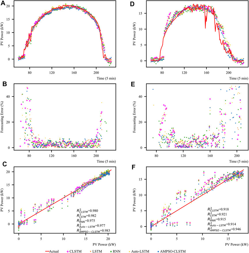
FIGURE 7. Forecasting result analysis for Alice Spring on a sunny day and a rainy day. (A,D) plot the observed PV power on the selected sunny and rainy days, respectively, as well as the predicted values for each model. (B,E) plot the percentage errors of the predicted values and the observed values. (C,F) plot the regression analyses for the sunny and rainy days.

The optimal network is obtained by decoding the optimal particles of fifty independent runs of the AMPSO-CLSTM and calculating the number of channels of the CNN and the number of hidden neurons of the LSTM in the corresponding neural network, as shown in Table 4. The model tends to choose a smaller number of channels in the convolutional layer and a smaller number of hidden neurons in the LSTM, despite the large maximum limits we gave in the hyperparameter settings (filter: 512, unit: 100). The number of channels decreases by 51.76–71.09%, while the number of LSTM hidden neurons decreases by 32–60% compared to the CLSTM model. Smaller numbers of channels and hidden neurons means that the network has higher versatility and that the network is less affected by overfitting.

TABLE 4

TABLE 4. Distribution of the structural hyperparameters for 50 independent runs on the DKASC data set.

In summary, the proposed model can provide good prediction results for different seasons and under different meteorological conditions. Accurate PV output power prediction can reduce the volatility and uncertainty of PV power generation and can ensure the safety of the power grid. Compared with other models, the proposed AMPSO-CLSTM model performs better in short-term PV power prediction, with higher accuracy and smaller error. The PV power prediction method based on deep learning can be applied to power grid operation management to reduce the loss caused by uncertainty.

Taiyangshan Photovoltaic Power Station

To verify the generalization ability of the proposed model, in this section, the model is tested on the Taiyangshan PV plant in Wuzhong, Ningxia, where is located in different geographical and meteorological conditions as well as different photovoltaic systems with Alice Springs. The data set contains operation data from January 1 to 31 December 2016, with a sampling interval of 15 min. The data consist of six main items: total radiation ($W/m^2$), module temperature (°C), ambient temperature (°C), air pressure ($hPa$), relative humidity (%) and actual power generated ($kW$). The technical specifications of this power system are shown in Table 5.

TABLE 5

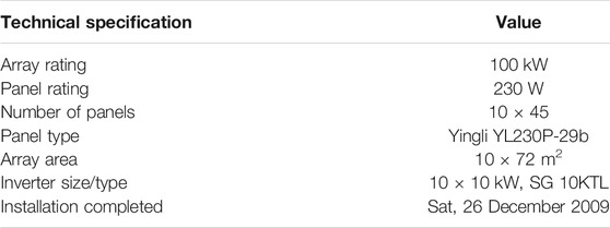
TABLE 5. Technical specifications of the Taiyangshan power system.

The main hyperparameters of the model are basically the same as in the previous paper, but the maximum number of CNN channels is adjusted to 256 to accommodate the smaller input dimensions and volume of the data. The method of data cleaning and weight initialization is the same as in the previous paper and thus will not be repeated here. Because we have only 1 year of operational data, the test data cannot cover all seasons; thus, the conventional data set partitioning method is chosen: 80% of the data are used for training the network, 10% for validation, and the remaining 10% for testing to measure the network performance. Similarly, 50 independent runs are performed for each of the models to verify the robustness. The error indexes for the results of the 50 independent runs are shown in Figure 8.

FIGURE 8

FIGURE 8. Boxplots of error indexes for 50 independent runs on the Taiyangshan data set. (A-C) respectively show the RMSE, MAE and MAPE of all models in case 2.

As shown in Figure 8, the proposed AMPSO-CLSTM model still has higher prediction accuracy and smaller fluctuation intervals than do the other models, even though the input dimensions, sampling resolution and data volume of this data set differ significantly from those of the data set used in the previous section. Note that the Auto-LSTM has a further decrease in accuracy on this data set, which is consistent with the point made in the previous section that the autoencoder has poorer results with lower input dimensions. Consistent with the previous operation, the results of 50 independent runs of the different models with the lowest RMSE are selected for comparison, and the errors on the test set are shown in Table 6. The proposed model still performs well on this data set, with the prediction results on the three error indexes being the smallest of all models. Hence, the model has some robustness and stability and is able to adapt to data of different size and input dimension.

TABLE 6

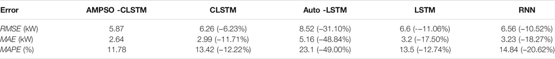
TABLE 6. PV power forecasting error.

The actual operational data available for this power station cover only 1 year; thus, the analysis in this section compares the network performance from a weather perspective only. Referring to local weather forecast and meteorological data, randomly selected sunny and rainy days from the test set are plotted in Figure 9. As shown in Figures 9A,D, all models obtain satisfactory results on this sunny day for this data set. During cloudy and rainy days in winter, the meteorological conditions change rapidly. Therefore, the fit of all models decreases. As shown in the figure, all the models are able to learn the general trend of the curve, except for Auto-LSTM, which did not fit the PV output power curve very well. In the winter season of Ningxia, the days are short, and the PV output power has more observations close to zero in the morning and at dusk. Figures 9B,E show that all models have higher forecast errors at dawn and dusk, while at other times of the day, the model’s forecast errors basically remain below 10%, which is the same as in the previous section. As shown in Figures 9C,F, the R² values of the different models are higher under clear weather conditions. The R² index of the proposed AMPSO-CLSTM is 0.981, which is slightly lower than that of the RNN. This result indicates that the various models are able to fit the curve well under sunny conditions. Compared with sunny days, the R² index of the prediction results of the various models on cloudy and rainy days decreases, but the R² index of the AMPSO-CLSTM model is 0.723, which is the highest among all the models. The AMPSO-CLSTM model is still able to explain 72.3% of the variation in PV output power in cloudy and rainy weather, which is more difficult to predict. In addition, the R² index of Auto-LSTM is negative on cloudy and rainy days. Under this kind of weather condition, the regression effect of Auto-LSTM is weaker than that of the mean model, which may be because the model does not have enough information to explain the changes in PV’ output power when the dimensions of the input factors are small and because the autoencoder structure of Auto-LSTM reduces the dimensions of the input data, which aggravates this information loss.

FIGURE 9

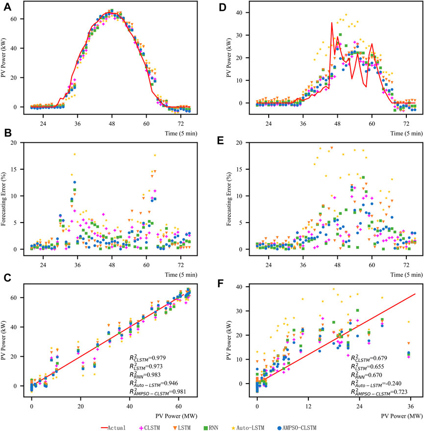
FIGURE 9. Forecasting result analysis for Taiyangshan on a sunny day and a rainy day. (A,D) are the forecasting results for Taiyangshan on a sunny day and a rainy day. (B,E) are the forecasting error of all models on a sunny day and a rainy day. (C,F) plot the regression analyses for the sunny and rainy day.

The optimal particles of AMPSO-CLSTM on the data set for 50 runs are decoded, and the number of CNN channels and number of hidden neurons of LSTM in the corresponding neural network are calculated. The structural parameters of 50 independent operations on the Taiyangshan data set are shown in Table 7. In the results of the AMPSO-CLSTM runs, the number of CNN channels decreases by 61.72–86.72%, while the number of LSTM hidden neurons decreases by 53–84% compared with the CLSTM model. The model has a larger decrease in structural parameters on this data set compared to that on the Alice Springs data set, which means that the model is able to adapt to input features with smaller dimensions and smaller samples and automatically scales down the network structure to match the data. Thus, the model is generalizable.

TABLE 7

TABLE 7. Network structure for 50 independent operations (Taiyangshan data set).

Conclusion

To solve the problem caused by the fluctuation and instability of PV power generation, this paper proposes a new CLSTM hybrid prediction model based on AMPSO. The proposed model combines the CNN and LSTM network of deep learning to effectively extract and fit high-dimensional features of PV power generation time series data and introduces the AMPSO algorithm to optimize the structure and weights of CLSTM at the same time to obtain the optimal structure and weight combination of the CLSTM network.

Next, several kinds of forecasting models (CLSTM, LSTM, RNN and Auto-LSTM) as long as the proposed AMPSO-CLSTM model are tested by using the PV power data of the Alice Spring PV system in Australia and the Taiyangshan PV power station in Wuzhong, Ningxia, China. The results show that compared with that of the existing models (CLSTM, LSTM, RNN and Auto-LSTM), the RMSE of the proposed PV power generation model on the two data sets decreases by 1.92–6.53% and 6.23–31.10%, the MAE decreases by 6.92–16.87% and 11.71–48.84%, and the MAPE decreases by 13.24–31.75% and 12.22–49.00%, respectively.

Compared with the CLSTM model, the optimized AMPSO-CLSTM model reduces the number of CNN channels by 51.76–71.09% and 61.72–86.72% and the number of LSTM hidden neurons by 32–60% and 53–84% on the two data sets, respectively. In different seasons and under different weather conditions, the proposed model has good prediction performance; hence, it can be applied to data with different seasonal meteorological index changes, factor dimensions, data sizes and sampling resolutions of PV power generation.

Data Availability Statement

The original contributions presented in the study are included in the article/Supplementary Materials, further inquiries can be directed to the corresponding author.

Author Contributions

SY: Conceptualization, Project administration, Writing‐original draft, Writing‐review and editing. RHn: Writing original draft, Writing-review and editing. YZ: Computing, Programming and Writing-original draft. CG: Writing‐review and editing.

Funding

Financial supports from the National Natural Science Foundation of China (No’s. 71822403, 31961143006, and 72174188) and Hubei Natural Science Foundation, China (No. 2019CFA089) are gratefully acknowledged.

Conflict of Interest

The authors declare that they have no known competing financial interests or personal relationships that could have appeared to influence the work reported in this paper.

Publisher’s Note

All claims expressed in this article are solely those of the authors and do not necessarily represent those of their affiliated organizations, or those of the publisher, the editors and the reviewers. Any product that may be evaluated in this article, or claim that may be made by its manufacturer, is not guaranteed or endorsed by the publisher.

Supplementary Material

The Supplementary Material for this article can be found online at: https://www.frontiersin.org/articles/10.3389/fenrg.2022.815256/full#supplementary-material

References

Abdel-Nasser, M., and Mahmoud, K. (2019). Accurate Photovoltaic Power Forecasting Models Using Deep LSTM-RNN. Neural Comput. Applic. 31, 2727–2740. doi:10.1007/s00521-017-3225-z

CrossRef Full Text | Google Scholar

Al-Dahidi, S., Ayadi, O., Adeeb, J., and Louzazni, M. (2019). Assessment of Artificial Neural Networks Learning Algorithms and Training Datasets for Solar Photovoltaic Power Production Prediction. Front. Energ. Res. 7, 130. doi:10.3389/fenrg.2019.00130

CrossRef Full Text | Google Scholar

Alfi, A. (2011). PSO with Adaptive Mutation and Inertia Weight and its Application in Parameter Estimation of Dynamic Systems. Acta Automatica Sinica. 37, 541–549. doi:10.1016/s1874-1029(11)60205-x

CrossRef Full Text | Google Scholar

Alkandari, M., and Ahmad, I. (2020). Solar Power Generation Forecasting Using Ensemble Approach Based on Deep Learning and Statistical Methods. Appl. Comput. Inform. ahead-of-print. doi:10.1016/j.aci.2019.11.002

CrossRef Full Text | Google Scholar

Bashir, Z. A., and El-Hawary, M. E. (2009). Applying Wavelets to Short-Term Load Forecasting Using PSO-Based Neural Networks. IEEE Trans. Power Syst. 24, 20–27. doi:10.1109/tpwrs.2008.2008606

CrossRef Full Text | Google Scholar

Bergstra, J., and Bengio, Y. (2012). Random Search for Hyper-Parameter Optimization. J. Machine Learn. Res. 13, 281–305. doi:10.5555/2188385.2188395

CrossRef Full Text | Google Scholar

Bouzerdoum, M., Mellit, A., and Massi Pavan, A. (2013). A Hybrid Model (SARIMA-SVM) for Short-Term Power Forecasting of a Small-Scale Grid-Connected Photovoltaic Plant. Solar Energy. 98, 226–235. doi:10.1016/j.solener.2013.10.002

CrossRef Full Text | Google Scholar

Buwei, W., Jianfeng, C., Bo, W., and Shuanglei, F. (2018). “A Solar Power Prediction Using Support Vector Machines Based on Multi-Source Data Fusion,” in 2018 International Conference on Power System Technology (POWERCON)), 4573–4577. doi:10.1109/powercon.2018.8601672

CrossRef Full Text | Google Scholar

Chai, M., Xia, F., Hao, S., Peng, D., Cui, C., and Liu, W. (2019). PV Power Prediction Based on LSTM With Adaptive Hyperparameter Adjustment. IEEE Access. 7, 115473–115486. doi:10.1109/access.2019.2936597

CrossRef Full Text | Google Scholar

Chan, L.-W., and Fallside, F. (1987). An Adaptive Training Algorithm for Back Propagation Networks. Computer Speech Lang. 2, 205–218. doi:10.1016/0885-2308(87)90009-x

CrossRef Full Text | Google Scholar

Chu, Y., Urquhart, B., Gohari, S. M. I., Pedro, H. T. C., Kleissl, J., and Coimbra, C. F. M. (2015). Short-term Reforecasting of Power Output from a 48 MWe Solar PV Plant. Solar Energy. 112, 68–77. doi:10.1016/j.solener.2014.11.017

CrossRef Full Text | Google Scholar

DKASC(Dka Solar Centre) (2020). Operation Data of the DKASC PV System in Alice Springs, Australia. Available at: http://dkasolarcentre.com.au/.

Google Scholar

Ghimire, S., Deo, R. C., Raj, N., and Mi, J. (2019a). Deep Solar Radiation Forecasting with Convolutional Neural Network and Long Short-Term Memory Network Algorithms. Appl. Energ. 253, 113541. doi:10.1016/j.apenergy.2019.113541

CrossRef Full Text | Google Scholar

Ghimire, S., Deo, R. C., Raj, N., and Mi, J. C. (2019b). Deep Learning Neural Networks Trained with MODIS Satellite-Derived Predictors for Long-Term Global Solar Radiation Prediction. Energies. 12, 2407. doi:10.3390/en12122407

CrossRef Full Text | Google Scholar

Glorot, X., and Bengio, Y. (2010). Understanding the Difficulty of Training Deep Feedforward Neural Networks. J. Machine Learn. Res. 9, 249–256. Available at: http://proceedings.mlr.press/v9/glorot10a/glorot10a.pdf

Google Scholar

Greff, K., Srivastava, R. K., Koutník, J., Steunebrink, B. R., and Schmidhuber, J. (2017). LSTM: A Search Space Odyssey. IEEE Trans. Neural Netw. Learn. Syst. 28, 2222–2232. doi:10.1109/tnnls.2016.2582924

PubMed Abstract | CrossRef Full Text | Google Scholar

Hafeez, G., Alimgeer, K. S., and Khan, I. (2020). Electric Load Forecasting Based on Deep Learning and Optimized by Heuristic Algorithm in Smart Grid. Appl. Energ. 269, 114915. doi:10.1016/j.apenergy.2020.114915

CrossRef Full Text | Google Scholar

Han, L., Jing, H., Zhang, R., and Gao, Z. (2019). Wind Power Forecast Based on Improved Long Short Term Memory Network. Energy 189, 116300. doi:10.1016/j.energy.2019.116300

CrossRef Full Text | Google Scholar

Huang, Y., Xiang, Y., Zhao, R., and Cheng, Z. (2020). Air Quality Prediction Using Improved PSO-BP Neural Network. IEEE Access 8, 99346–99353. doi:10.1109/access.2020.2998145

CrossRef Full Text | Google Scholar

IRENA(International Renewable Energy Agency). (2021). Renewable Capacity Statistics 2021. Abu Dhabi: International Renewable Energy Agency (IRENA). Available at: https://www.irena.org/-/media/Files/IRENA/Agency/Publication/2021/Apr/IRENA_RE_Capacity_Statistics_2021.pdf

Google Scholar

Iversen, E. B., Morales, J. M., Møller, J. K., Trombe, P.-J., and Madsen, H. (2017). Leveraging Stochastic Differential Equations for Probabilistic Forecasting of Wind Power Using a Dynamic Power Curve. Wind Energy 20, 33–44. doi:10.1002/we.1988

CrossRef Full Text | Google Scholar

Jing, S., Qu, X., and Zeng, S. (2011). Short-Term Wind Power Generation Forecasting: Direct versus Indirect Arima-Based Approaches. Int. J. Green Energ. 8, 100–112. doi:10.1080/15435075.2011.546755

CrossRef Full Text | Google Scholar

Khandakar, A., E. H. Chowdhury, M. M., Khoda Kazi, M., Benhmed, K., Touati, F., Al-Hitmi, M., et al. (2019). Machine Learning Based Photovoltaics (PV) Power Prediction Using Different Environmental Parameters of Qatar. Energies 12, 2782. doi:10.3390/en12142782

CrossRef Full Text | Google Scholar

Kim, T. Y., and Cho, S. B. (2019). “Particle Swarm Optimization-Based CNN-LSTM Networks for Forecasting Energy Consumption,” in 2019 IEEE Congress on Evolutionary Computation (CEC)), 1510–1516.

CrossRef Full Text | Google Scholar

Lecun, Y., Bengio, Y., and Hinton, G. (2015). Deep Learning. Nature 521, 436–444. doi:10.1038/nature14539

PubMed Abstract | CrossRef Full Text | Google Scholar

Li, P., Zhou, K., Lu, X., and Yang, S. (2020). A Hybrid Deep Learning Model for Short-Term PV Power Forecasting. Appl. Energ. 259, 114216. doi:10.1016/j.apenergy.2019.114216

CrossRef Full Text | Google Scholar

López, E., Valle, C., Allende, H., Gil, E., and Madsen, H. (2018). Wind Power Forecasting Based on Echo State Networks and Long Short-Term Memory. Energies 11, 526. doi:10.3390/en11030526

CrossRef Full Text | Google Scholar

Luo, X., Zhang, D., and Zhu, X. (2021). Deep Learning Based Forecasting of Photovoltaic Power Generation by Incorporating Domain Knowledge. Energy 225, 120240. doi:10.1016/j.energy.2021.120240

CrossRef Full Text | Google Scholar

Mamun, A. A., Hoq, M., Hossain, E., and Bayindir, R. (2019). “A Hybrid Deep Learning Model with Evolutionary Algorithm for Short-Term Load Forecasting,” in 2019 8th International Conference on Renewable Energy Research and Applications (ICRERA)), 886–891. doi:10.1109/icrera47325.2019.8996550

CrossRef Full Text | Google Scholar

Marion, B., Anderberg, A., Deline, C., Cueto, J. D., Muller, M., Perrin, G., et al. (2014). “New Data Set for Validating PV Module Performance Models,” in 2014 IEEE 40th Photovoltaic Specialist Conference (PVSC)), 1362–1366.

CrossRef Full Text | Google Scholar

Mcculloch, W. S., and Pitts, W. (1943). A Logical Calculus of the Ideas Immanent in Nervous Activity. Bull. Math. Biophys. 5, 115–133. doi:10.1007/bf02478259

CrossRef Full Text | Google Scholar

Nam, K., Hwangbo, S., and Yoo, C. (2020). A Deep Learning-Based Forecasting Model for Renewable Energy Scenarios to Guide Sustainable Energy Policy: A Case Study of Korea. Renew. Sustainable Energ. Rev. 122, 109725. doi:10.1016/j.rser.2020.109725

CrossRef Full Text | Google Scholar

Narendra, K. S., and Parthasarathy, K. (1989). “Adaptive Identification and Control of Dynamical Systems Using Neural Networks,” in Proceedings of the 28th IEEE Conference on Decision and Control), 17371732–17371738.

Google Scholar

Nargesian, F., Samulowitz, H., Khurana, U., Khalil, E. B., and Turaga, D. S. (2017). “Learning Feature Engineering for Classification,” in Proceedings of the Twenty-Sixth International Joint Conference on Artificial Intelligence, 2529–2535.

CrossRef Full Text | Google Scholar

Neshat, M., Nezhad, M. M., Abbasnejad, E., Mirjalili, S., Tjernberg, L. B., Astiaso Garcia, D., et al. (2021). A Deep Learning-Based Evolutionary Model for Short-Term Wind Speed Forecasting: A Case Study of the Lillgrund Offshore Wind Farm. Energ. Convers. Management. 236, 114002. doi:10.1016/j.enconman.2021.114002

CrossRef Full Text | Google Scholar

Qing, X., and Niu, Y. (2018). Hourly Day-Ahead Solar Irradiance Prediction Using Weather Forecasts by LSTM. Energy. 148, 461–468. doi:10.1016/j.energy.2018.01.177

CrossRef Full Text | Google Scholar

Rumelhart, D. E., Hinton, G. E., and Williams, R. J. (1986). Learning Representations by Back-Propagating Errors. Nature. 323, 533–536. doi:10.1038/323533a0

CrossRef Full Text | Google Scholar

Shahid, F., Zameer, A., and Muneeb, M. (2021). A Novel Genetic LSTM Model for Wind Power Forecast. Energy. 223, 120069. doi:10.1016/j.energy.2021.120069

CrossRef Full Text | Google Scholar

Shaker, H., Manfre, D., and Zareipour, H. (2020). Forecasting the Aggregated Output of a Large Fleet of Small Behind-The-Meter Solar Photovoltaic Sites. Renew. Energ. 147, 1861–1869. doi:10.1016/j.renene.2019.09.102

CrossRef Full Text | Google Scholar

Taiyangshan, W. (2016). Wuzhong Taiyangshan PV Power Station Annual Report. WuZhong, China: Taiyangshan Photovoltaic Power Station.

Google Scholar

Tang, J., and Zhao, X. (2009). “Particle Swarm Optimization with Adaptive Mutation,” in 2009 WASE International Conference on Information Engineering), 234–237.

CrossRef Full Text | Google Scholar

Trigo-González, M., Batlles, F. J., Alonso-Montesinos, J., Ferrada, P., Del Sagrado, J., Martínez-Durbán, M., et al. (2019). Hourly PV Production Estimation by Means of an Exportable Multiple Linear Regression Model. Renew. Energ. 135, 303–312. doi:10.1016/j.renene.2018.12.014

CrossRef Full Text | Google Scholar

Unfccc, C. (2015). Paris Agreement. Bonn: FCCCC/CP/2015/L. 9/Rev. 1.

Google Scholar

Vaitheeswaran, S. S., and Ventrapragada, V. R. (2019). “Wind Power Pattern Prediction in Time Series Measuremnt Data for Wind Energy Prediction Modelling Using LSTM-GA Networks,” in 2019 10th International Conference on Computing, Communication and Networking Technologies (ICCCNT)), 1–5. doi:10.1109/icccnt45670.2019.8944827

CrossRef Full Text | Google Scholar

Wang, H., Wang, W., and Wu, Z. (2013). Particle Swarm Optimization with Adaptive Mutation for Multimodal Optimization. Appl. Mathematics Comput. 221, 296–305. doi:10.1016/j.amc.2013.06.074

CrossRef Full Text | Google Scholar

Wang, K., Qi, X., and Liu, H. (2019a). A Comparison of Day-Ahead Photovoltaic Power Forecasting Models Based on Deep Learning Neural Network. Appl. Energ. 251, 113315. doi:10.1016/j.apenergy.2019.113315

CrossRef Full Text | Google Scholar

Wang, K., Qi, X., and Liu, H. (2019b). Photovoltaic Power Forecasting Based LSTM-Convolutional Network. Energy 189, 116225. doi:10.1016/j.energy.2019.116225

CrossRef Full Text | Google Scholar

Xiong, S., Zhou, H., He, S., Zhang, L., Xia, Q., Xuan, J., et al. (2020). A Novel End-To-End Fault Diagnosis Approach for Rolling Bearings by Integrating Wavelet Packet Transform into Convolutional Neural Network Structures. Sensors 20, 4965. doi:10.3390/s20174965

PubMed Abstract | CrossRef Full Text | Google Scholar

Xu, X., and Zhong, T. (2006). Construction and Realization of Cubic Spline Interpolation Function. Ordnance Industry Automation. 25, 76–78. doi:10.3969/j.issn.1006-1576.2006.11.034

CrossRef Full Text | Google Scholar

Yona, A., Senjyu, T., Funabashi, T., and Kim, C.-H. (2013). Determination Method of Insolation Prediction With Fuzzy and Applying Neural Network for Long-Term Ahead PV Power Output Correction. IEEE Trans. Sustain. Energ. 4, 527–533. doi:10.1109/tste.2013.2246591

CrossRef Full Text | Google Scholar

Zang, H., Liu, L., Sun, L., Cheng, L., Wei, Z., and Sun, G. (2020). Short-term Global Horizontal Irradiance Forecasting Based on a Hybrid CNN-LSTM Model with Spatiotemporal Correlations. Renew. Energ. 160, 26–41. doi:10.1016/j.renene.2020.05.150

CrossRef Full Text | Google Scholar

Zhang, C., Liang, M. M., Song, X. G., Liu, L. X., Wang, H., Li, W. S., et al. (2022). Generative Adversarial Network for Geological Prediction Based on TBM Operational Data. Mech. Syst. Signal Process. 162, 108035. doi:10.1016/j.ymssp.2021.108035

CrossRef Full Text | Google Scholar

Zhang, C., Zhang, Y., Su, J., Gu, T., and Yang, M. (2020). Performance Prediction of PV Modules Based on Artificial Neural Network and Explicit Analytical Model. J. Renew. Sustainable Energ. 12, 013501. doi:10.1063/1.5131432

CrossRef Full Text | Google Scholar

Zhang, J., Verschae, R., Nobuhara, S., and Lalonde, J.-F. (2018). Deep Photovoltaic Nowcasting. Solar Energy 176, 267–276. doi:10.1016/j.solener.2018.10.024

CrossRef Full Text | Google Scholar

Zhou, Y., Zhou, N., Gong, L., and Jiang, M. (2020). Prediction of Photovoltaic Power Output Based on Similar Day Analysis, Genetic Algorithm and Extreme Learning Machine. Energy. 204, 117894. doi:10.1016/j.energy.2020.117894

CrossRef Full Text | Google Scholar

Glossary

AMPSO adaptive mutation particle swarm optimization

ANN artificial neural networks

$b$ bias

BP back propagation

$c$ learning factor

CNN convolutional neural network

CLSTM convolutional long short-term memory network

DBN deep belief network

DKASC desert knowledge Australia solar centre

ESN echo state network

ELM extreme learning machine

$fit\left(P_m\right)$ fitness of particle m

$F$ channels of the CNN

GA genetic algorithm

GAN generative adversarial network

$gbest$ population optimal position

$gen$ current iteration

MAE mean absolute error

MAPE mean absolute percentage error

$max\_gen$ upper limit of the number of iterations

MLP multilayer Perceptron

$pbes{t}_m$ the best position that the particle has reached

PV photovoltaic power

PSO particle swarm optimization

$R$ the number of input convolution mapping

RNN recurrent neural network

RMSE root mean square error

$S$ step of the predicted time

SVM support vector machine

SAE stacked auto-encoder

$U$ unit of the LSTM

$v$ particle velocity

$w$ weight

$\otimes$ convolution operation

$z_g^l$ the kth convolution mapping of layer l

$\sigma$ activation function

${\omega }_m$ adaptive inertia weight of particle m