Smart EV Charging Strategies Based on Charging Behavior

Coming years, the number of electric vehicles (EVs) shall increase significantly, so the demand for electricity for charging EVs will proportionately increase as well. Thus, the growing energy requirements for charging these EVs might put huge burden on the electricity generation and supply infrastructure. Such a huge load growth opportunity for utilities if integrated successfully, or if not, a significant challenge to operate and balance grid loads in the future. Customarily, the increase in adoption of EVs in recent years has yielded challenges to the utilities as the electricity demand of EVs occurs mostly during peak hours. In some cases, a sojourn time may be longer than a charging time, that means, EVs will be connected to the charging station without charging. However, the load shifting potential of EVs may be consequential and might subsequently be used to alleviate challenges to the electric grid system. Considering charging behaviors for EV scheduling is crucial, as they depend on uncertainties of EV availabilities (i.e., sojourn time and energy required). Such uncertainties would impact substantially on the deployment of feasible EV charging scheduling. To address above-mentioned issues, firstly, we define an idle time ratio, which is basically load shifting potential. Consequently, we develop a heuristic EV charging scheduling scheme with an emphasis on inevitable charging behaviors of the EV users. Such a scheduling incorporates priority determination using the idle time ratio and TOU period as well as priority-based time slot allocation. Moreover, accurate prioritization of EVs is realized by predicting the energy demand and idle time ratio. Minimization of charging cost is perhaps the most perceptive objective, such that, the EV charging scheduling is done when TOU tariff is low. Performance evaluation shows that the proposed flexible smart charging scheduling outperforms the baseline scheduling in terms of the charging power and charging cost.

1 Introduction

Currently, over 1.27 million Electric vehicles (EVs) have been adopted in the United States; by 2030, about 20 million EVs are anticipated on the United States roads.

Moreover, EVs play critical role in the Smart cities as they do not yield CO₂ emission, in turn, decarbonizing road transportation. As urban population shifts toward more sustainable energy future, the steady growth of EVs is anticipated.

As the number of EVs increases, the demand for electricity for charging EVs will increase as well. Thus, the growing energy requirements for charging EVs might put huge burden on the electricity generation and supply infrastructure. Such a huge load growth could yield either opportunity forthe utilities if integrated successfully, or significant challenges to operate and balance grid loads in the future. The high penetration of EVs may have a substantial impact on the stability of the electric grid; particularly, when uncoordinated EV charging is employed. With the uncoordinated charging, EVs shall immediately start charging upon their arrival with the maximum charging power until their charging targets are completed.

Smart charging of EVs is one of the appealing approaches, which has the potential to alleviate the challenges to the electric grid by shifting the charging load to a low demand period. This would not only foster demand response management but also decrease investments needed in the EV charging infrastructure. Thus, it can be means for reducing EV charging cost to the EV users.

Most EV charging activities take place in residential areas, commercial areas (i.e., shopping complex, public parking), and workplaces. Due to the longer sojourn time than the charging time, Electric Vehicle Supply Equipment (EVSEs) are occupied longer than needed (i.e., EVs are connected without charging), that may cause under utilization. Nevertheless, the load shifting potential of EVs may be consequential and might subsequently be used to alleviate challenges to the electric grid system.

Furthermore, considering charging behaviors for EV scheduling is crucial, as they depend on uncertainties of EV availabilities (i.e., sojourn time and energy required). Such uncertainties would impact substantially on the deployment of feasible EV charging scheduling.

In order to address such issues of user charging behavior uncertainties, initially, we define an idle time ratio, which is basically load shifting potential. Consequently, this paper intends to develop a heuristic EV charging scheduling scheme with an emphasis on inevitable charging behaviors of the EV users. Such a scheduling incorporates priority determination using the idle time ratio and TOU period as well as priority-based time slot allocation. Moreover, accurate prioritization of EVs is realized by predicting the energy demand and idle time ratio. Minimization of charging cost is perhaps the most perceptive objective, such that, the EV charging scheduling is done when TOU tariff is low.

The remainder of this paper is organized as follows. Section 2 describes related works while Section 3 highlights preliminaries. Analysis of EV charging sessions and charging behavior is described in Section 4. Proposed flexible smart charging strategies are depicted in Section 5. Finally, conclusions and future work are presented in Section 6.

2 Related Works

Numerous studies have been conducted on the EV charging scheduling problem (Zeng et al., 2021). Basically, EV charging scheduling can be mainly categorized into two categories: centralized and decentralized approaches (Alsabbagh and Ma, 2020). In centralized approach, the charging station operator or the aggregator determines the charging schedule for all EVs to achieve an optimal solution. Whereas, in decentralized approach, EVs can determine the charging time and charging power, that means, a decision is made at the node level. These EVs shall have coordination with the aggregator which may act independently or cooperatively with other aggregators. Prior works on smart charging deal with various objectives such as minimizing energy costs, maximizing profit, and stabilizing power load (Wu et al., 2020).

In (Zhang et al., 2020), viewing charging preferences of different types of users, a comprehensive satisfaction degree model was set up to obtain different users’ charging strategies. And Time-Of-Use (TOU) pricing strategy for EV charging was proposed that considers the demand response and realizes the effective dispatch of EV charging load based on price signals.

Generally, EV charging demands are characterized by 3-tuple including arrival time, departure time and the requested charging energy. Due to the user charging behavior uncertainties, one or more of the parameters may be undetermined, for instance, the arrival time (Wu et al., 2020), departure time (Frendo et al., 2021), and energy consumption (Chung et al., 2019).

The paper (Clairand et al., 2020) aims to perform an assessment of various strategies based on different input parameters as well as conducts stochastic analyses using Monte Carlo simulations to evaluate the impact of such input parameters, in which uncertainties such as hour of charging and required energy are considered. Similarly, in (Fotouhi et al., 2019), the authors depicted a stochastic model that takes into consideration the EV drivers’ behavioral characteristics in terms of their response to the EV battery charge level when deciding to charge or disconnect at a charging station.

In (Zeng et al., 2021), the authors proposed a station-level optimization framework to operate charging station with optimal pricing policy and charge scheduling. Such a model incorporates human behaviors in efficient charging decision process.

In smart charging, predictions of charging behavior uncertainties would be beneficial when they are integrated with EV charging scheduling. Typically, forecasting is realized with a regression model trained on historical data to predict upcoming data. For instance, the paper (Shahriar et al., 2021) depicts the usage of historical data along with weather, traffic information to predict EV session duration and energy consumption using support vector regression (SVR), random forest (RF), XGBoost and Deep neural networks.

Similarly, in (Chung et al., 2019), the authors investigated several machine learning algorithms including SVR, RF and diffusion-based kernel density estimator (DKDE) to predict charging behavior, including stay duration and energy consumption based on historical data. And they proposed Ensemble Predicting Algorithm (EPA) to enhance predicting performance by decreasing 11% of the stay duration and 22% of the energy consumption prediction errors.

The authors addressed dynamic EV charging problems with two objectives: minimizing the total charging cost and minimizing the peak load. They proposed online EV charge scheduling approaches such as greedy algorithm and prediction-based charging strategy to focus on above-mentioned objectives (Wu et al., 2020).

Additionally, the EVs parked in the parking lots of the workplaces can provide substantial charging flexibility due to the long sojourn time (Sadeghianpourhamami et al., 2018). As a finding shows that on an average, only 20% of the total connection time is used for charging the EVs, smart charging strategies and optimization of the charging sessions are essential (Bouhassani et al., 2019).

In (Lucas et al., 2019), the authors applied regression methods such as RF, Gradient Boosting, and XGBoost to estimate the idle time of EV at the charging infrastructure Similarly, the authors (Gerritsma et al., 2019) proposed a method for analyzing the time-dependent flexibility of EV demand. Basically, such a flexibility is influenced by charging power, EV characteristics, and other environmental factors. Their results depict that 59% of the aggregated EV demand can be delayed for more than 8h, and 16% for even more than 24 h.

In(Canigueral and Melendez, 2021), the methodology was proposed to address scheduling problem, and optimizing each user profile according to its suitable flexibility objective, since the classification of EV sessions among generic user profiles can be used by aggregators to deliver smart charging in a more efficient and robust manner.

Likewise, in the paper (Sun et al., 2019), the authors proposed an online mechanism to aim integrating the multi-dimensional flexibility in the EV coordinated charging problem, and exploiting the energy-flexibility and deadline-flexibility by modeling the valuations of each EV’s charging request (i.e., energy demand, arrival time and deadline) as a function of the required energy demand and deadline.

Furthermore, the authors not only developed a parameterized aggregated plugin EV charging model using the energy boundaries to express the charging flexibility but also proposed to parameterize the aggregated charging policy (Long et al., 2021). And the paper (Wu et al., 2021) highlighted a method for evaluating the charging and discharging scheduling potential of electric vehicles considering the uncertainty in the users’ responses in case of occasional operation of a power grid.

Some prior works focused on the use of prioritization in the smart charging. For instance, in (Frendo et al., 2021), the authors employed regression models trained on historical data to predict individual EV departure time and then incorporated this prediction in an EV charging scheduling heuristic approach in order to maximize fair share among EVs by prioritizing for equal chances of reaching a sufficient state of charge by the departure time.

Most of the recent prior works either assume perfect information about the EV user charging behavior uncertainties or just consider the 3-tuple EV charging demand parameters (Frendo et al., 2021). In this work, we have considered EV user charging behavior uncertainties including energy consumption and an idle time ratio (i.e., time-dependent flexibility). Moreover, we not only incorporate a regression model for predicting such uncertainties but also employ such predictions for priority determination and ultimately, deploy heuristic priority-based EV charging scheduling. Even though such a charging flexibility would be beneficial for bi-directional EV charging, in this work, we have not considered Vehicle-to-grid (V2G).

3 Preliminaries

3.1 Charging Transaction

A charging transaction is characterized by three important parameters.

• Connection time: It is the time interval between starting and ending a connection to an EVSE. It is essentially a sojourn time.

• Charging time: It is the time an EV is actually charging.

• Charging Power: It is max power that the EVSE can offer to charge the EV for that transaction.

Some EV users may plug in and leave their vehicles for an extended period at public EV designated parking lots. Thus, idle time can be determined by the period when EVs remain at such parking spots without charging.

On one hand, prolonged idle time may be a concern for other EV users who need to charge their vehicles to complete their planned trips. On other hand, if the connection time is longer than the charging time, which means that the charging session provides flexibility to shift a charging session to a later moment.

3.2 EV Rates

There can be two main kinds of electric tariffs: Flat and Time-of-Use (TOU). A flat tariff is a flat rate constant over the entire year and, at any time of the day the electricity price is the same. A TOU rate not only varies within a day but also depends on seasons and days. During defined periods of the day, electricity prices are higher than during the rest of the day. High prices periods are called “on-peak periods” and lower prices periods are called “off-peak periods.”

There are several dedicated tariff plans to charge EVs (Lee et al., 2020). One of them is Southern California Edison (SCE) tariff, which includes various schemes such as TOU-EV-7, TOU-EV-8, and TOU-EV-9. These plans are applied for charging of the EVs such that these TOU periods incentivize EV users to optimize their charging patterns to minimize electricity costs.

In this study, we have considered the use of SCE TOU-EV plan (Southern California Edison, 2019). In this regard, EV users having charging demands up to 20 kW can use TOU-EV-7 tariff plan, whereas those having charging demands from 20 to 500 kW require to use TOU-EV-8 plan.

As SCE TOU-EV plan, TOU periods are defined as follows, which is presented in Table 1.

TABLE 1

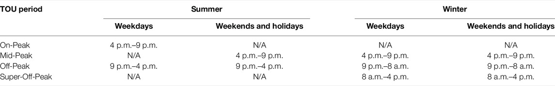
TABLE 1. SCE TOU-EV TOU plan.

Summer season is from June to September, whereas winter season is from October to May.

3.3 Clustering Mechanism

Clustering is an unsupervised machine learning technique that divides the data points into several groups or clusters based on their attributes or features such that data points in the same groups are more like other data points in the same group and dissimilar to the data points in other groups.

One of the widely-used unsupervised learning approaches based on distance-based algorithm is K-Means. Since K-means algorithm is dependent on initialization of centroids, it may result in poor clustering. K-Means++ can overcome the shortcomings of K-Means such that the former ensures a smarter initialization of the centroids and improves the quality of the clustering.

Gaussian Mixture Model (GMM) is a probabilistic model that assumes all the data points are generated from a mixture of a finite number of Gaussian distributions with unknown parameters. The first visible difference between K-Means and GMM is the shape the decision boundaries. GMMs are somewhat more flexible and with a covariance matrix we can make the boundaries elliptical, as opposed to circular boundaries with K-means.

Gaussian Mixture is a function that is comprised of several Gaussians, each identified by k ∈ 1, …, K, where K is the number of clusters of our dataset. Each Gaussian k in the mixture is comprised of the following parameters:

• A mean μ that defines its centre.

• A covariance Σ that defines its width. This would be equivalent to the dimensions of an ellipsoid in a multivariate scenario.

• A mixing probability π that defines how big or small the Gaussian function will be.

Like most clustering methods, the number of desired clusters must be specified before fitting the model. The number of clusters specifies the number of components in the GMM.

It can be thought of mixture models as generalizing K-Means clustering to incorporate information about the covariance structure of the data as well as the centers of the latent Gaussians. Thus, GMM can be applied in a similar way to K-Means++, but there are some major differences between these two algorithms. GMM is better than K-Means++ as it does account for variance too.

4 Analysis of EV Charging Sessions and Charging Behavior

4.1 Datasets

4.1.1 Data Collection

In this work, the original data was obtained through ElaadNL (ElaadNL, 2020), which is a Dutch smart charging knowledge center promoted by a grid operators consortium.

The Transaction dataset consists of a set of 10-tuple elements: Transaction ID, ChargePoint ID, Connector ID, UTC Transaction Start, UTC Transaction Stop, Start Card, Connected Time, Charge Time, Total Energy, and Max Power. Whereas the Metervalues dataset consists of a set of 7-tuple elements: Transaction ID, ChargePoint ID, Connector ID, UTC Time, Collected Value, Energy Interval, and Average Power.

4.1.2 Data Processing

Before analysis, some of the data were excluded; charging sessions having connection time more than 24 h were excluded. These instances occurred mainly due to technical difficulties where EV users were unable to properly connect their vehicles to the port. Such instances account for 2.1% of the total sessions. In total, 9,800 charging sessions were analyzed to investigate the charging behavior.

4.2 Preliminary Analysis

4.2.1 Total Energy with Respect to Time of Day

Figures 1A–C show total energy with respect to time of day during all seasons, summer, and winter, respectively.

Corresponding to the charging transaction trend during all seasons, as shown in Figure 1A), there are two major peaks at 7 a.m. and 4 p.m., and one minor peak at 10 a.m. It can be seen that during daytime, total energy (kWh) remains high, whereas during night time it is low.

Similar patterns can be observed during summer and winter as depicted in Figures 1B,C, respectively. Only difference is that during summer, major peaks occur at 6 a.m. and 3 p.m. and during winter, minor peak is at 11 a.m.

FIGURE 1

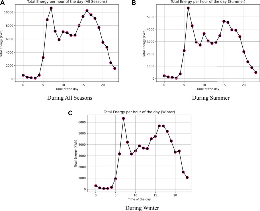
FIGURE 1. Total energy with respect to time of day for various seasons.

4.2.2 Average Idle Time Ratio With Respect to Time of Day

An idle time ratio can be defined as the ratio of idle time to sojourn time. Basically it is a measure of load shifting potential and can be viewed as smart charging potential (Bouhassani et al., 2019) or time-dependent flexibility (Gerritsma et al., 2019).

Figures 2A–C show average idle time ratio with respect to time of day during all seasons, summer, and winter, respectively.

FIGURE 2

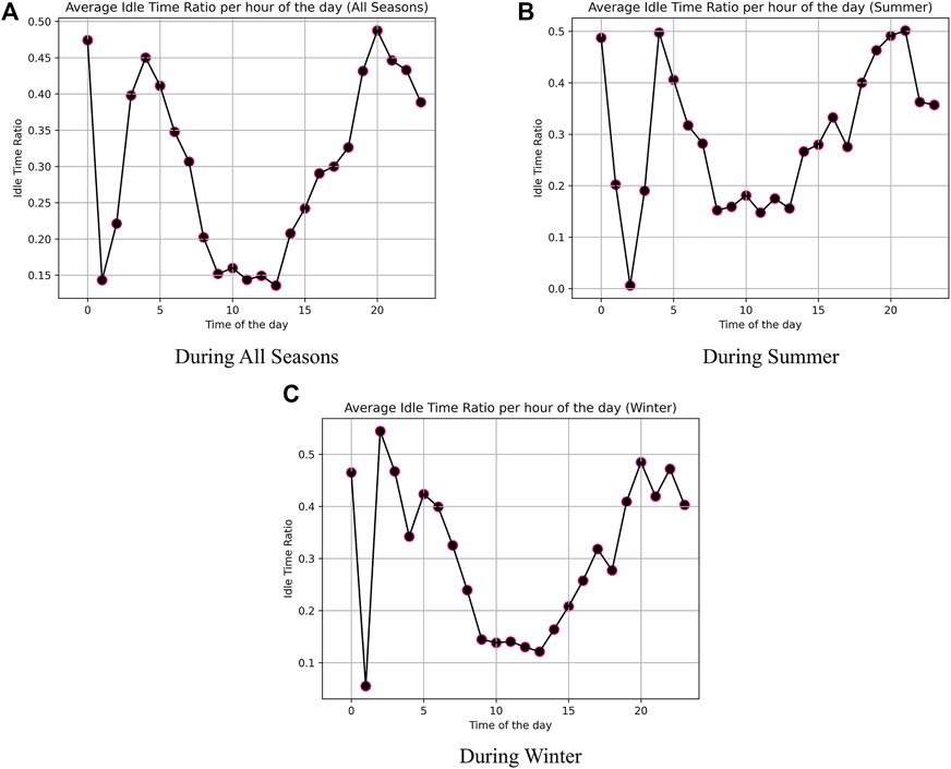
FIGURE 2. Average idle time ratio with respect to time of day for various seasons.

As shown in Figure 2A, during all seasons, an average idle time ratio is low during day time, especially between 9 a.m. and 1:30 p.m., while during the night, higher average idle time ratio is concentrated, with exception of a deep at 1 a.m. It can be observed that higher average idle time ratio indicates that the charging flexibility is high, that means during that period, the charging activity may be deferred.

Similar patterns can be observed during summer and winter as depicted in Figures 2B,C, respectively.

4.3 Analysis of Clustering EV Charging Behavior

In this work, various cluster GMM formation was analyzed before selecting the best cluster formation number.

Applying the Akaike’s Information Criteria (AIC)/Bayesian Information Criterion (BIC) criterion, the number of components in a Gaussian Mixture can be selected in an efficient manner. As the number of components is increased, the AIC and BIC values decrease. At a certain point, the value of the AIC/BIC does not change significantly anymore. The number of clusters at which this occurs is the optimum number of clusters that should be used. In this research work, the four clusters identified are based on the value of the AIC/BIC.

After obtaining optimal number of components, we then train the model on the dataset with number of components 4 and 5. Under the GMM, the clustered data points for different value of n_comp are shown in Figure 3. It can seen that in Figure 3A, there are 4 clusters in total which are visualized in different colors and in Figure 3B, there are 5 clusters in total which are visualized in different colors.

FIGURE 3

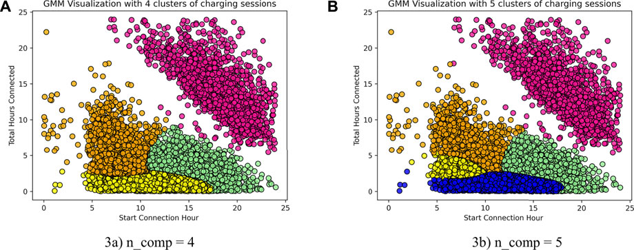
FIGURE 3. GMM visualization for various clusters.

4.4 Cluster Labeling for Charging Sessions

Cluster labeling is the problem of picking descriptive, human-readable labels for the clusters produced by a document clustering algorithm; standard clustering algorithms do not typically produce any such labels.

Clusters of charging transactions can be found based on two variables: the time at which a charging transaction starts and the total connection time. Based on these two variables, we can label the different clusters. For that purpose, we have selected GMM Visualization with 4 clusters.

Clustering labelling of charging sessions is important for the visualization of EV charging behavior as shown in Figure 4. Each cluster of sessions can be considered as a homogeneous group that has the similar characteristics.

FIGURE 4

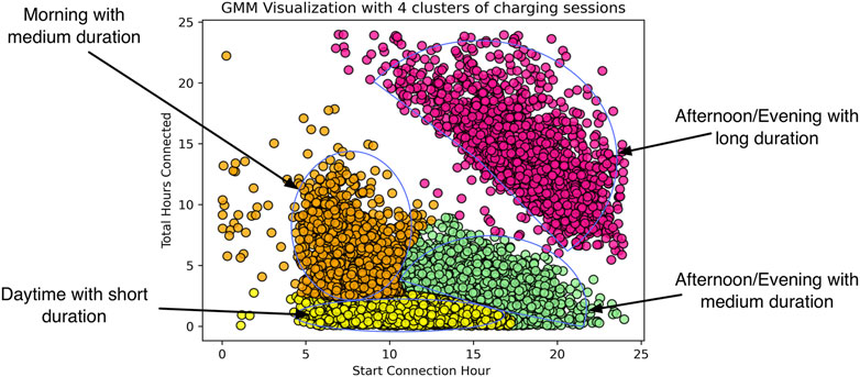
FIGURE 4. GMM clustering with labeling.

4.4.1 Morning Hour With Medium Duration (MMD)

Morning with medium duration (MMD) includes charging sessions starting in the morning for average connection duration of 8.5 h. It can be also called “Work and Charge.”

For instance, MMD mainly includes charging at the workplaces.

Such a charging provides moderate flexibility for the system.

4.4.2 Daytime With Short Duration (DSD)

Daytime with short duration (DSD) comprises the charging sessions may commerce throughout the day with relatively short duration, i.e., average of 1.5 h. It can be also called “Stop and Charge.”

For example, DSD includes electric taxi, visitors, car sharing.

Such a charging provides minimum flexibility for the system.

4.4.3 Afternoon/Evening With Medium Duration (AEMD)

Afternoon/evening with medium duration (AEMD) includes charging sessions starting in the afternoon or the evening having average duration of 4.5 h. It can be also called “Park and Charge.”

For instance, AEMD includes charging at shopping centers, eating places (restaurants, bar) and recreation centres (movie theatre, physical fitness).

Such a charging provides some flexibility for the system.

4.4.4 Afternoon/Evening With Long Duration (AELD)

Afternoon/evening with long duration (AELD) includes charging sessions starting in the afternoon or the evening having average duration of 15 h. It can be also called “Home and Charge.”

For instance, charging at home is an example of AELD.

Such a charging provides the highest flexibility for the system.

4.5 Predictive Analysis of EV User Behavior

This subsection discusses the regression methods for EV user behavior prediction. The main goal is to predict EV users’ energy demand and idle time ratio based on the historical charging data when their EVs are being charged.

4.5.1 Regression Algorithms

Regression models depict the relationship between a target (output) variable, and one or more predictor (input) variables. Several regression algorithms such as Support Vector Regression (SVR), Decision Trees, Random Forest, and Least-Squares Boosting (LSBoost) can be considered. We have selected Random Forest and LSBoost to predict the idle time ratio and energy consumption for the EV charging scheduling.

4.5.1.1 Random Forest

Random Forest (RF) is an ensemble learning technique, which is commonly used for both classification and regression problems. Its main idea is to use of multiple decision trees, like a forest. Initially, the algorithm starts with a number of bootstrap samples from the original data. Each of these samples will generate a decision tree with an adjusting operation, in which afterwards several predictors are randomly sampled. The algorithm goes on choosing the best split from the group of the sampled variables, instead of considering them all. The square root of the total number of variables is assumed by the algorithm as the default number of the predictors’ value.

4.5.1.2 Least-Squares Boosting

LSBoost is one of boosting algorithms under regression ensembles. Such an ensemble method, which uses the least squares as the loss criteria, fits to minimize mean-squared error. At every step, the ensemble endows a new learner to the difference between the observed response and the aggregated prediction of all learners grown previously. With a given learning rate η ∈ [0, 1], the ensemble may fit each incoming learner to y_n − ηf (x_n), where y_n is the observed response and f (x_n) is the aggregated prediction from all weak learners grown so far for observation x_n.

4.5.2 Model Accuracy Evaluation

For the purpose of evaluating model performance, model accuracy evaluation metrics are used to evaluate and compare the above-mentioned machine learning algorithms.

To assess the prediction accuracy, various performance indicators are utilized as the root mean square error (RMSE), mean absolute error (MAE), and the coefficient of determination, R².

• Coefficient of determination (R²). It represents the proportion of the variance in the dependent variable which is explained by the linear regression model. It is a scale-free score, the value of R square will be less than one.

• Mean Absolute Error (MAE). It represents the average of the absolute difference between the actual and predicted values in the dataset. It measures the average of the residuals in the dataset.

• Root Mean Square Error (RMSE). It is the square root of mean squared error, that is the average of the squared difference between the original and predicted values in the dataset. It measures the standard deviation of residuals.

Basically, idle time ratio and energy consumption are evaluated.

In case of idle time ratio, the final dataset was formed with the ten variables, including: six numeric independent variables—total energy, max charging power, charge time, transaction start time, transaction stop time, and Connector ID; four categorical independent variables—EVSE ID, seasons, TOU period, and week of the day; and, idle time ratio, the numeric response variable.

Similarly, in case of energy consumption, the final dataset was formed with the ten variables, including: six numeric independent variables—max charging power, charge time, idle time ratio, transaction start time, transaction stop time, and Connector ID; four categorical independent variables—EVSE ID, seasons, TOU period, and week of the day; and, total energy, the numeric response variable.

Hyperparameter tuning refers to the shaping of the model architecture by searching the right hyperparameter to find high precision and accuracy. There are several parameter tuning techniques, two of the most widely used parameter optimiser techniques including Random search and Grid search can be considered. In this study, we have used Random search cross validation (CV) method provided by the scikit-learn library. Two main parameters must be input for this exercise to be carried out and which determine its accuracy and time: the number of iterations (n_iter) and the Cross Validation (cv). In this study, n_iter: 100 (candidates) and cv: 10 (folds) were used.

After performing hyperparameter tuning, optimized hyperparameters are obtained for each method.

For Random Forest, optimized hyperparameters used are as follows: “n_estimators”: 500; “max_depth”: 60; “min_samples_split”: 7; “min_samples_leaf”: 2; “max_features”: “sqrt”; and “bootstrap”: True.

For LSBoost, optimized hyperparameters used are as follows: “min_samples_leaf”: 2; “learning_rating”: 0.1.

Table 2 provides the model accuracy evaluation metrics of each algorithm in terms of the R², RMSE, and MAE.

The lower value of MAE and RMSE implies higher accuracy of a regression model, whereas a higher value of R² is considered desirable.

It can be observed that LSBoost has achieved the best accuracy in predicting the idle time ratio with low RMSE of 0.034, low MAE of 0.023 and high R² of 0.97 for all seasons. Similarly, the LSBoost provides the best prediction values for the summer and winter seasons.

Likewise, in case of the energy consumption, for all scenarios, the LSBoost regression method yields the highest R² score and the lowest MAE and RMSE.

Figure 5 shows the prediction outcomes with the LSBoost regression.

TABLE 2

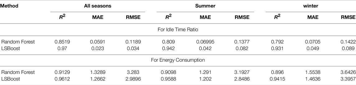
TABLE 2. Metric evaluation with respect to idle time ratio and energy consumption.

FIGURE 5

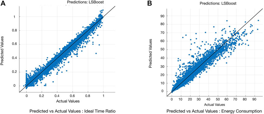
FIGURE 5. Prediction outcomes with the LSBoost regression for Idle Time Ratio and Energy Consumption.

Figure 5A depicts predicted values vs. actual values for the idle time ratio while Figure 5B illustrates predicted values vs. actual values for the energy consumption. Both cases have relatively high prediction accuracy.

5 Flexible Smart Charging Strategies

In this section, we present a charge scheduling algorithm to find optimal solutions.

5.1 System Model

Considering an EV charging network that is controlled and managed by a Centralized Controller (CC) along with charging station (CS) local controllers (LCs). The purpose of CC is to provide updated TOU plan and to minimize the peak load in the distribution system.

In such an EV charging infrastructure, EVSEs are distributed in various locations such as commercial, workplaces, and residentials (i.e., condos) in the particular area. Each location has LC for managing its EVSEs. And the CC is used for managing and coordinating all the LCs. The participating EV users need to subscribe to the system in order to participant in recharging activities.

Whenever recharging is required, the EV user can initiate a charging session by sending a charging request through his Mobile Apps.

Consider a set of EVs i ∈ N. Each EV i operates with a battery characterised by its maximum capacity B_i (kWh) and its state of charge SoC_i defined as the available capacity and expressed as a percentage of its nominal capacity B_i. $So{C}_i\in [So{C}_{{\min }_i},So{C}_{{\max }_i}]$, where $So{C}_{{\max }_i}$ and $So{C}_{{\max }_i}$ are the minimal and the maximal allowable values of SoC, respectively. SoC_i is bounded as depicted in Eq. 1.

$So{C}_{{min}_i}\le So{C}_i\le So{C}_{{max}_i}(1)$

Upon arrival, an EV i sends a charging request to the CS local controller. Such a charging request has a 3-tuple of parameters, \{ $t_{a{r}_i},t_{d{e}_i},So{C}_i^{ini}$ \}, which can be used to describe a charging behavior. Here, $t_{a{r}_i}$ is arrival time, $t_{d{e}_i}$ is a departure time, and initial SoC is $So{C}_i^{ini}$. It should be noted that $t_{a{r}_i}<t_{d{e}_i}$.

The time horizon is divided into time slots, t = {1, … , T}, each of length Δt represents the time interval [t − 1, t]. In order words, Δt is a time duration between two consecutive meter readings.

Time slots can be in either charging period or idle period depending upon whether EV i performs its charging task at a given time slot t. Thus, we define a binary variable x_i,t that can be expressed as in Eq. 2.

$x_{i,t}=\left\{\begin{array}{cc}1\hfill & \mathrm{i}\mathrm{f}\mathrm{c}\mathrm{o}\mathrm{n}\mathrm{n}\mathrm{e}\mathrm{c}\mathrm{t}\mathrm{e}\mathrm{d}\mathrm{a}\mathrm{n}\mathrm{d}\mathrm{c}\mathrm{h}\mathrm{a}\mathrm{r}\mathrm{g}\mathrm{i}\mathrm{n}\mathrm{g}\mathrm{s}\mathrm{u}\mathrm{c}\mathrm{h}\mathrm{t}\mathrm{h}\mathrm{a}\mathrm{t}{P}_i>0,\mathrm{i}.\mathrm{e}.,\mathrm{c}\mathrm{h}\mathrm{a}\mathrm{r}\mathrm{g}\mathrm{i}\mathrm{n}\mathrm{g}\mathrm{p}\mathrm{e}\mathrm{r}\mathrm{i}\mathrm{o}\mathrm{d},\hfill \\ 0\hfill & \mathrm{i}\mathrm{f}\mathrm{i}\mathrm{s}\mathrm{c}\mathrm{o}\mathrm{n}\mathrm{n}\mathrm{e}\mathrm{c}\mathrm{t}\mathrm{e}\mathrm{d},\mathrm{b}\mathrm{u}\mathrm{t}\mathrm{n}\mathrm{o}\mathrm{t}\mathrm{c}\mathrm{h}\mathrm{a}\mathrm{r}\mathrm{g}\mathrm{i}\mathrm{n}\mathrm{g}\mathrm{s}\mathrm{u}\mathrm{c}\mathrm{h}\mathrm{t}\mathrm{h}\mathrm{a}\mathrm{t}{P}_i=0,\mathrm{i}.\mathrm{e}.,\mathrm{i}\mathrm{d}\mathrm{l}\mathrm{e}\mathrm{p}\mathrm{e}\mathrm{r}\mathrm{i}\mathrm{o}\mathrm{d},\hfill \end{array}\right.(2)$

The connection time for transaction k of the EV i is the period during which an EV is plugged in to an EVSE, which is given using Eq. 3.

${\Upsilon }_i=t_{a{r}_i}-t_{d{e}_i}(3)$

If EV i is assigned to EVSE j, then at each time period t, EVSE j may provide a charging power P_it to EV i. Typically, the maximum charging power is equivalent to the minimum of the maximum charging power allowed for the EV battery, and the maximum charging power of the EVSE. Furthermore, for unidirectional charging, the lower bound is equal to zero; that means, a discharging process shall not be occurred.

Thus, the charging power of an EV battery is bounded, which can be given as in Eq. 4.

$0\le P_{i_t}\le P_i^{max},\forall i\in N,t\in T(4)$

Depending on the charging power P_i and charging efficiency η of EV i, the time required to charge EV i can be computed as in Eq. 5.

${\mathrm{\Gamma }}_i=\frac{{\mathrm{\Theta }}_i^{req}{B}_i}{P_i\eta }(5)$

Considering the binary charging variable x_i,t, the charged time can be derived by counting the number of non-zero values for average power [kW] during transaction k, as expressed in Eq. 6.

${\mathrm{\Gamma }}_i=\sum _{t=1}^T\left(x_{i,t}\mathrm{\Delta }t\right)(6)$

It should be noted that the charged time should be less or equal to the connection time, i.e., Γ_i ≤ ϒ_i.

While charging with charging power $P_{i_t}$, the EV i retrieves an amount of energy in the time period t, which is given as in Eq. 7.

${\mathrm{\Theta }}_{i_t}=P_{i_t}\mathrm{\Delta }t\eta (7)$

Thus, ${\mathrm{\Theta }}_{i_t}$, (kWh) is the energy transfer to a EV i in each charging stage.

Energy demand [kWh], which is the total energy during charging transaction k, can be formulated as in Eq. 8.

${\mathrm{\Theta }}_i=\sum _{t=1}^T\left(x_{it}{\mathrm{\Theta }}_{i_t}\right)(8)$

Let’s assume the predicted energy demand be ${\mathrm{\Theta }}_i^{dem}$, then the actual energy demand should not exceed the predicted energy demand and is scheduled within SoC limits, i.e., ${\mathrm{\Theta }}_i<={\mathrm{\Theta }}_i^{dem}$ and $So{C}_i^{ini}+{\mathrm{\Theta }}_i<=So{C}_{{max}_i}$. This constraint guarantees that the EVSE meets an EV’s energy need during the connection time.

5.2 Charging Strategies

5.2.1 Instant Strategy

Instant charging strategy allows vehicles to charge immediately. That means, it is assumed that an EV is plugged in to an EVSE as soon as it arrives at a charge station and start charging immediately. The vehicle keeps charging until the battery is fully charged or unplugged by the EV user.

5.2.2 Allotted-Slot Strategy

In allotted-slot strategy, a charging session is divided into smaller time slots and allotted over the total connected time. Such a strategy has the potential for large fleets, where immediate access to charging is unnecessary.

5.2.3 Deferred Strategy

Deferred strategy selects the charging schedule based on time-of-use (TOU) tariff rates and EV user’s schedule. That means, a charging session is shifted to the off-peak time period. Deferred strategy can selectively charge the vehicle at lower TOU rate as much as possible at each charge event. Typically, it can be utilized for relatively long-term parking. This strategy employs required energy and schedule information to maximize the cost benefit for EV users and reduce grid peak demand.

5.3 Flexible Smart EV Charging

The charging parameters including the energy consumption and idle time ratio play crucial role on EV charging scheduling to determine an optimal solution. Fundamentally, when an EV user initiates a charging session, the prediction of idle time ratio and energy consumption could provide positive impact on determining charging slot allocation scheduling.

Let binary variable w_i,t denote whether EV i ∈ N is assigned for charging at an EVSE j ∈ J at time slot t ∈ T.

$w_{i,t}=\left\{\begin{array}{cc}1\hfill & \forall i\in N,t\in T\hfill \\ 0\hfill & \text{Otherwise},\hfill \end{array}\right.(9)$

Considering the charging network service capability, at most M EVs can be charged concurrently. Therefore, during each time slot, the total number of EVs being charged should satisfy Eq. 10.

$\sum _{i=1}^N\left(w_{i,t}\right)\le M(10)$

Average Idle time ratio for charging transaction k of the EV i is given by

${\mathrm{\Psi }}_i=\frac{{\Upsilon }_i-{\mathrm{\Gamma }}_i}{{\Upsilon }_i}(11)$

So, Ψ can be viewed as a measure of flexibility in load shifting for a given charging session. As per the Elaad dataset, it can be observed that there are about 45% of charging transactions having Ψ = 0, whereas about 55% of charging transactions have Ψ > 0 including 28% of charging sessions having Ψ > 0.5.

Basically, smart charging with flexibility depends on charging behavior of the EV users. For instance, some EV users are willing to leave the charging station immediately after charging activity is completed. While some remain connected to the EVSE without charging even after the completion of charging activity.

Furthermore, some EV users want to have fully charging, i.e., Θⁱ = SoC_max. Whereas some want only partial charging i.e., Θⁱ < SoC_max.

If the value of Ψ is larger, then it is likely to have more the flexibility in EV charging.

Typically, amount of flexibility in EV charging depends on following factors:

• Time-of-use (TOU) plans

• Driving range capabilities of EVs

• Recharging opportunities during day or night time for convenience and availability

By considering the TOU tariff, shifting the load to the TOU period with lower rates can reduce the charging cost significantly.

Having TOU rate and average charging rate at time slot t, the charging cost for EV i can be derived as.

$C_u=\sum _{t=1}^T\left(r_t\mathrm{\Delta }t{P}_{i_t}\eta \right)(12)$

One of the objectives of flexible smart charging is to charge the EV at a given charging transaction at as low TOU rates as possible to minimize the charging cost.

The objective function is expressed in Eq. 13 as a charging cost minimization problem for all the EVs.

$\begin{array}{cc}\hfill C_m=& \min \sum _{i=1}^N\left(C_{u_i}\right)\hfill \\ \hfill \text{subject\hspace{0.17em}to}\end{array}(13)$

$\begin{array}{ccc}\hfill & \hfill & So{C}_{{min}_i}\le So{C}_i\le So{C}_{{max}_i}\hfill \end{array}(14)$

$\begin{array}{ccc}\hfill & \hfill & 0\le P_{i_t}\le P_i^{max},\hfill \end{array}(15)$

The constraint Eq. 14 shows that SOC should be within the allowable limit, and the constraint Eq. 15 determines the limit for charging power.

We now introduce a heuristic approach to address above-mentioned problem. The proposed effective flexible smart charging strategy comprises of behavioral load shifting approach based on recharging priority. Such a priority not only depends on charging behavior including energy demand and idle time ratio but also considers the TOU plan. Thus, it can allow the system to selectively charge EVs at the lower TOU rates as much as possible.

The local controller in conjunction with the centralized controller determines the flexible charging process to schedule feasible charging session for each EV. In the first stage, the system can predict the energy demand and idle time ratio for an incoming EV using regression model trained on historical data. In the second stage, with the given TOU plan and predicted idle time ratio, the system can determine priority to each EV. In the final stage, using above-mentioned priorities and energy demand, the system can optimally schedule timeslots to the EVs in order to minimize the charging cost.

Figure 6 depicts flow chart for flexible smart charging scheme that includes three stages as mentioned above.

FIGURE 6

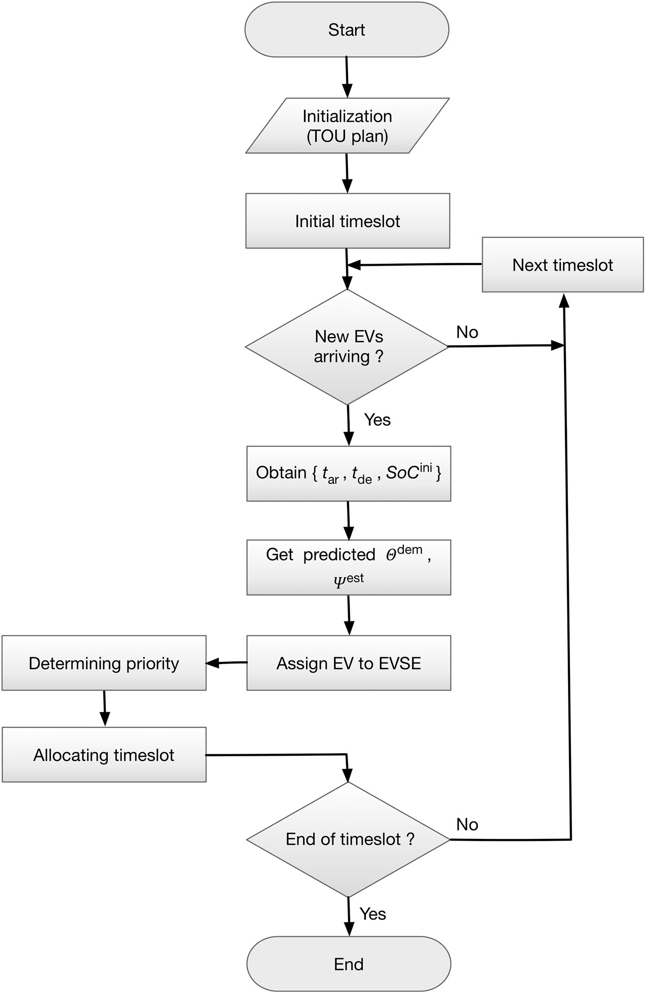
FIGURE 6. Flow chart for flexible smart charging scheme.

As depicted in Figure 6, the attributes such as arrival time, departure time and initial SoC shall be known upon arrival of each EV. Then the system employs regression model trained on historical data to predict the energy demand and idle time ratio.

Fundamentally, the proposed flexible smart charging scheme is based on two major modules–1) Priority determination module, and 2) Timeslot allocation module.

Figure 7 shows various modules in the proposed scheme. Priority determination and timeslot allocation modules are depicted in Figures 7A,B respectively.

In the priority determination module, two priority variables are considered–one for determination of recharging urgency, which is influenced by two parameters–idle time ratio and TOU period and another for minimization of charging cost, which considers of TOU period along with TOU rate. Thus, this scheme provides one of the appropriate scheduling approaches for EV charging.

As per SCE TOU plan, a session either summer or winter (ses ∈ {sum, win}) may have different TOU periods. Now, let us derive all possible subsets of TOU periods, which are as follows.

$\begin{array}{cc}\hfill {\mathrm{\Omega }}_1^{ses}& =\left\{{\mathrm{\Omega }}_{to{u}_1}^{ses}\right\}\hfill \\ \hfill {\mathrm{\Omega }}_2^{ses}& =\left\{{\mathrm{\Omega }}_{to{u}_2}^{ses}\right\}\hfill \\ \hfill {\mathrm{\Omega }}_3^{ses}& =\left\{{\mathrm{\Omega }}_{to{u}_3}^{ses}\right\}\hfill \\ \hfill {\mathrm{\Omega }}_4^{ses}& =\left\{{\mathrm{\Omega }}_{to{u}_1}^{ses},{\mathrm{\Omega }}_{to{u}_3}^{ses}\right\}\hfill \\ \hfill {\mathrm{\Omega }}_5^{ses}& =\left\{{\mathrm{\Omega }}_{to{u}_2}^{ses},{\mathrm{\Omega }}_{to{u}_3}^{ses}\right\}\hfill \\ \hfill {\mathrm{\Omega }}_6^{ses}& =\left\{{\mathrm{\Omega }}_{to{u}_1}^{ses},{\mathrm{\Omega }}_{to{u}_2}^{ses}\right\}\hfill \\ \hfill {\mathrm{\Omega }}_7^{ses}& =\left\{{\mathrm{\Omega }}_{to{u}_1}^{ses},{\mathrm{\Omega }}_{to{u}_2}^{ses},{\mathrm{\Omega }}_{to{u}_3}^{ses}\right\}\hfill \\ \hfill & \mathrm{w}\mathrm{h}\mathrm{e}\mathrm{r}\mathrm{e},\mathrm{f}\mathrm{o}\mathrm{r}sum:{tou}_1=\mathrm{o}\mathrm{n}-\mathrm{p}\mathrm{e}\mathrm{a}\mathrm{k};{tou}_2=\mathrm{m}\mathrm{i}\mathrm{d}-\mathrm{p}\mathrm{e}\mathrm{a}\mathrm{k};{tou}_3=\mathrm{o}\mathrm{f}\mathrm{f}-\mathrm{p}\mathrm{e}\mathrm{a}\mathrm{k};\hfill \\ \hfill & \mathrm{f}\mathrm{o}\mathrm{r}win:{tou}_1=\mathrm{m}\mathrm{i}\mathrm{d}-\mathrm{p}\mathrm{e}\mathrm{a}\mathrm{k};{tou}_2=\mathrm{o}\mathrm{f}\mathrm{f}-\mathrm{p}\mathrm{e}\mathrm{a}\mathrm{k};{tou}_3=\mathrm{s}\mathrm{u}\mathrm{p}\mathrm{e}\mathrm{r}-\mathrm{o}\mathrm{f}\mathrm{f}-\mathrm{p}\mathrm{e}\mathrm{a}\mathrm{k}.\hfill \end{array}(16)$

In case of the summer season, only two TOU periods can be existed at a time, for instance, during weekdays, on-peak and off-peak, and during weekends, mid-peak and off-peak. Thus, for the summer season, only subsets from ${\mathrm{\Omega }}_1^{ses}$ to ${\mathrm{\Omega }}_5^{ses}$ are valid. Whereas the winter season can have three TOU periods, namely, mid-peak, off-peak and super-off-peak, thus, all of the subsets are valid.

The priority that reflects the urgency to recharge can be denoted by Π_α depends upon the decision variables α_k: k ∈ {1, 2, 3}.

${\alpha }_1=\left\{\begin{array}{cc}1\hfill & \text{if}\mathrm{\Psi }=0,\text{\hspace{0.17em}and\hspace{0.17em}}\forall {\mathrm{\Omega }}_y^{ses}:y=\left\{\mathrm{1,2},\dots ,7\right\},\hfill \\ 0\hfill & \text{Otherwise}\hfill \end{array}\right.(17)$

${\alpha }_2=\left\{\begin{array}{cc}1\hfill & \text{if}\mathrm{\Psi }>0,\text{\hspace{0.17em}and\hspace{0.17em}}\forall {\mathrm{\Omega }}_y^{ses}:y=\left\{\mathrm{1,2,3}\right\}\hfill \\ 0\hfill & \text{Otherwise}\hfill \end{array}\right.(18)$

${\alpha }_3=\left\{\begin{array}{cc}1\hfill & \text{if}\mathrm{\Psi }>0,\text{\hspace{0.17em}and\hspace{0.17em}}\forall {\mathrm{\Omega }}_y^{ses}:y=\left\{\mathrm{4,5,6,7}\right\}\hfill \\ 0\hfill & \text{Otherwise}\hfill \end{array}\right.(19)$

As shown in Figure 7, the recharging urgency priority Π_α is set according to the decision variable α_k. For instance, when α₁ is 1, Π_α is 3, that means, the recharging urgency priority is the highest. And when α₃ is 1, Π_α is 1, that means, the recharging urgency priority is the lowest.

FIGURE 7

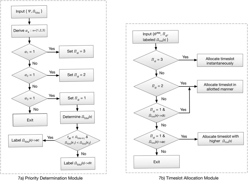
FIGURE 7. Priority determination and timeslot allocation modules in the proposed scheme.

The recharging urgency priority Π_α depends on the accuracy of the predicted value of Ψ, That is, the more accurate Ψ_est is, the more precisely EVs can be prioritized.

As per the SCE TOU-EV-8 plan, TOU period may have different TOU tariff. We shall assign a priority to TOU period $({\mathrm{\Omega }}_{to{u}_x}^{ses})$, which can be expressed as follows: ${\mathrm{\Omega }}_{to{u}_x}^{ses}(x),x\in \{\mathrm{1,2,3}\}$.

Here, higher the value of x, higher the TOU priority. That means, in summer season, off-peak has the highest priority, whereas on-peak has the lowest. Similarly, in the winter season, super-off-peak has the highest priority, whereas mid-peak has the lowest.

Furthermore, in case of α₃ = 1, ${\mathrm{\Omega }}_{to{u}_x}^{ses}(x)$ shall be labeled as ascending ${\mathrm{\Omega }}_{to{u}_x}^{ses}(x)\to ac$ when the following two conditions are met.

$\left\{\begin{array}{cc}{t}_{ar}\in {\mathrm{\Omega }}_{to{u}_{x_1}}^{ses}\hfill & \hfill \\ {\mathrm{\Omega }}_{to{u}_{x_1}}^{ses}\left(x_1\right)<{\mathrm{\Omega }}_{to{u}_{x_2}}^{ses}\left(x_2\right),\hfill & \forall x_1,x_2=\left\{\mathrm{1,2,3}\right\}\hfill \end{array}\right.(20)$

If above conditions are not satisfied, then it shall be labeled as descending ${\mathrm{\Omega }}_{to{u}_x}^{ses}(x)\to dc$.

In timeslot allocation module, ${\mathrm{\Pi }}_{\alpha }\text{and\hspace{0.17em}labelled\hspace{0.17em}}{\mathrm{\Omega }}_{to{u}_x}^{ses}(x)$ are used as input values. When {Π_α = 3}, then timeslots are allocated instantaneously. And if {Π_α = 2}, then timeslots are allocated in allotted manner. Then if the conditions $\{{\mathrm{\Pi }}_{\alpha }=1\&{\mathrm{\Omega }}_{to{u}_x}^{ses}(x)\to dc\}$ meet, then timeslots are allocated in allotted manner as well. In such a case, even though the load shifting is possible, the charging cost would not be minimized. Finally if the conditions $\{{\mathrm{\Pi }}_{\alpha }=1\&{\mathrm{\Omega }}_{to{u}_x}^{ses}(x)\to ac\}$ meet, then the minimization of the charging cost is possible while performing load shifting from lower TOU priority to higher TOU priority.

Furthermore, we characterize the instantaneous timeslot allocation as instant strategy, timeslot allocation in allotted manner as allotted-slot strategy, and timeslot allocation with higher TOU priority as deferred strategy.

5.3.1 Performance Evaluation and Results

We extensively evaluate the performance of the proposed smart charging mechanism. For this purpose, a real-world dataset from the Elaad is employed. And we have adopted SCE TOU-EV-8 for TOU plan as mentioned in Section 3.

We have considered two scenarios–one for summer season and another for winter season. In both scenarios, the EV charging network includes 30 EVSEs in the workplace. The deployed EVSEs are three-phase Level 2 chargers with maximum charging power of 11 kW. The whole day is equally divided into T = 96 time slots, with each slot duration as Δt = 15 min.

To assess the proposed flexible charging strategy, a baseline scheduling, which is exclusively based on first come, first served (FCFS) scheduling, is considered such that a comparison between two scheduling mechanisms can be conducted.

We have used MATLAB R2020a not only to pre-process the historical data and generate regression models but also to simulate the EV charging environment.

With historical data of the participated EVs, the system can generate regression models, which shall be used to predict the energy consumption and idle time ratio for the EVs.

We assume that 50 EVs randomly arriving to the workplace. For the convenience, they are homogenous having same battery capacity (B_i = 40 kWh) and charging efficiency (η = 1). And the minimum and maximum SoC are set to 20 and 90%, respectively. Moreover, the initial SoC for the EV must be at least min SoC.

The outcomes for different scheduling mechanisms in summer season is illustrated in Figure 8. Figure 8A depicts the charging power for baseline scheduling and flexible smart scheduling in summer season, while Figure 8B shows charging cost for baseline scheduling and flexible smart scheduling in summer season.

FIGURE 8

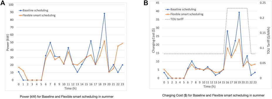
FIGURE 8. Outcomes for different scheduling mechanisms in summer.

From Figure 8A, with baseline scheduling, a major peak at 7 p.m. and two minor peaks (one at 7 a.m.; another at 4 p.m.) can be observed. These peaks occur due to either people are arriving to the work or leaving from the work. Furthermore, it can be observed that there no charging activities occur between 1 a.m. and 5 a.m. Using the flexible smart scheduling, these peaks are flattened by shifting some loads to the Off-peak TOU period. Particularly, the peak occuring at 7 p.m., which lies in the On-peak TOU period, is reduced significantly. It can be noticed that no load can be shifted to the time between 2 and 5 a.m. as people are not staying at the workplace after 2 a.m.

From Figure 8B, it can be observed that the proposed flexible smart charging scheme can achieve good output for reducing charging costs in comparison to the baseline scheduling scheme, since the former can significantly reduce charging cost during mid-peak TOU periods. More specifically, the proposed flexible smart charging scheme can reduce the total charging cost at 19 h by about 40%.

The outcomes for different scheduling mechanisms in winter season is illustrated in Figure 9. Figure 9A depicts the charging power for baseline scheduling and flexible smart scheduling in winter season, while Figure 9B shows charging cost for baseline scheduling and flexible smart scheduling in winter season.

FIGURE 9

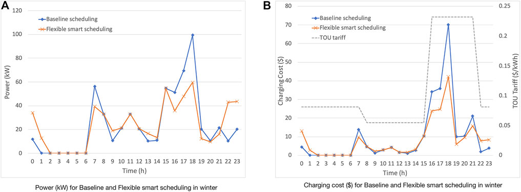
FIGURE 9. Outcomes for different scheduling mechanisms in winter.

5.4 Case Studies

In this sub-section, we have conducted case studies on the existing real-time charging transactions and analysis of the impact of the proposed flexible smart charging scheme.

This is done based on historical charging data from Elaad and an optimization criterion based on flexible smart charging scheme, in which SCE TOU plan is applied to determine TOU priority.

In order to study an impact of a charging behavior, we have selected some representive charging transactions for different EVs in the winter season from the Elaad dataset. As shown in Figure 10, each charging transaction has own charging pattern. For instance, the start time of some charging transaction are in the morning hour, while others in the evening. Likewise, some have long charging period, while some have long idle period.

FIGURE 10

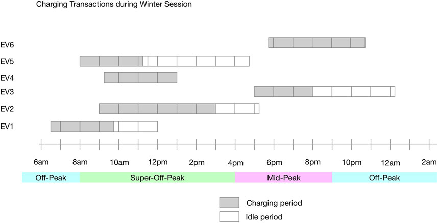
FIGURE 10. Charging transactions for different EVs in winter.

For instance, EV1, which arrives at 6:30 a.m. and departs at the noon, has connection and charged time of 5 h 30 min and 3 h 15 min, respectively. Thus, the EV1 is connected without charging for 2 h 15 min, in turn Ψ = 0.41. Likewise, as the arrival and departure time of EV3 are 5 p.m. and 0:15 a.m., respectively, it has connection and charged time of 7 h 15 min and 3 h, respectively. Thus, the EV3 is connected without charging for 4 h 15 min, in turn Ψ = 0.59. In such cases, load shifting is possible for minimizing charging cost.

EV4 that arrives at 9:15 a.m. and departs at 1 p.m. has same connection and charged time of 3 h 45 min. Similarly, EV6 that arrives at 6:45 p.m. and departs at 22:45 p.m. has same connection and charged time of 4 h. Since both EV4 and EV6 leave immediately after the completion of charging activities, Ψ = 0.

EV2 has connection time and charged time of 8 h 15 min and 6 h, respectively. Thus, the EV2 is connected but not charging for 2 h 15 min, in turn Ψ = 0.28. Similarly, EV5 has connection time and charged time of 8 h 45 min and 3 h 15 min, respectively. Thus, the EV5 is connected but not charging for 5 h 30 min, in turn Ψ = 0.63. In such cases, even though load shifting is possible, it cannot yield charging cost reduction. It can.

In general, with higher ratio of Ψ, more flexible will be EV charging such that the load in TOU period with higher tariff can be shifted to that with lower tariff.

We have selected some of the representative charging transactions for different seasons from Elaad datasets. Fundamentally, 20 charging transactions for summer season and 20 for winter season.

Table 3 depicts charging transactions during different seasons. Each charging transaction contains Transaction ID, ϒ_i, Γ_i, and Ψ_i.

TOU period distribution of charging time in summer for various scheduling mechanisms is shown in Figure 11. Figure 11A depicts such distribution for baseline scheduling, whereas Figure 11B depicts such distribution for flexible smart charging scheduling.

TABLE 3

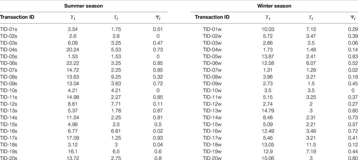
TABLE 3. Charging transactions during different seasons.

FIGURE 11

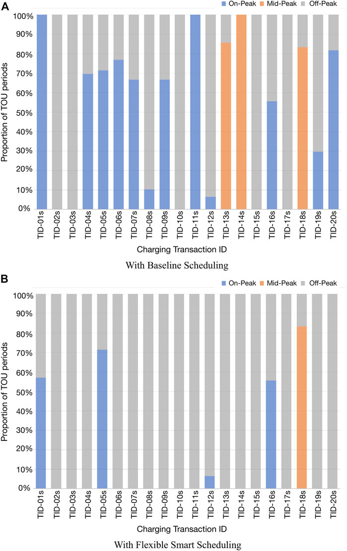
FIGURE 11. TOU period distribution of charging time in summer for various scheduling mechanisms.

It can be observed that with higher Ψ, charging transactions have greater charging flexibility such that charging load can be deferred to the time slots with higher TOU priority. For instance, in TID-11s, for baseline scheduling, all the charging sessions lie in the on-peak TOU period. Then, after applying the flexible smart charging, all the charging sessions have been deferred to the off-peak TOU period.

In case of TID-01s, about 43% of charging time slots have been deferred to the off-peak TOU period from the on-peak TOU period upon applying the flexible smart charging.

If Ψ is zero, then there is no charging flexibility. In such a case, the instant strategy is applied, for instance, TID-02s, TID-05s and TID-10s.

TOU period distribution of charging time in winter for various scheduling mechanisms is depicted in Figure 12. Such distribution for baseline scheduling is depicted in Figure 12A, whereas such distribution for flexible smart charging scheduling is depicted in Figure 12B.

FIGURE 12

FIGURE 12. TOU period distribution of charging time in winter for various scheduling mechanisms.

Similarly, during winter season, charging transactions having higher Ψ have greater charging flexibility so charging load can be deferred to the time slots with higher TOU priority. For instance, in TID-13w, for baseline scheduling, all the charging sessions lie in the mid-peak TOU period. Then, after applying the flexible smart charging, all the charging sessions have been deferred to the super-off-peak TOU period.

In case of TID-16w, 64% of charging time slots have been deferred to the off-peak TOU period from the mid-peak TOU period upon applying the flexible smart charging.

In TID-05w, initially, the TOU period distribution of charging time was 50% for mid-peak and 50% for off-peak. Then after employing the flexible smart charging, charging time slots have been deferred such that the TOU period distribution of charging time is changed to 100% for super-off-peak.

In case of TID-18w, initially, the TOU period distribution of charging time was about 44% for mid-peak, 39% for off-peak and 17% for super-off-peak. Upon employing the flexible smart charging, the TOU period distribution of charging time became about 28% for mid-peak, 54% for off-peak and 17% for super-off-peak.

If Ψ is zero, then there is no charging flexibility. In such a case, the instant strategy is applied, for instance, TID-10w.

Finally, the most appropriate smart charging strategy for each cluster label is determined. Instant charging strategy is suitable for the cluster label with Daytime with short duration (DSD) since it has smaller value of Ψ. While slot-allotted strategy can be applied for the cluster label with Morning hour with medium duration (MMD) as MMD may have only one TOU period even though MMD has higher value of Ψ. Deferred charging strategy with flexible load shifting is the best suited to the cluster label with Afternoon/evening with long duration (AELD) since it has the highest value of Ψ. It can be applied to the cluster label with Afternoon/evening with medium duration (AEMD) as AEMD spans between 11 a.m. and mid-night as well as moderate value of Ψ.

6 Conclusion and Future Work

This paper establishes a novel approach to address issues of user charging behavior uncertainty for EV charging scheduling by utilizing historical data.

Firstly, we have not only analyzed the real-time data from the ElaadNL to obtain user charging behavior such as energy consumption and idle time ratio but also used machine learning algorithms (i.e., GMM) to cluster them according to the charging behavior and then labeled them. Furthermore, we have used regression models (i.e., RF, LSBoost) to predict those user charging behavior parameters.

Secondly, we have proposed a heuristic EV charging scheduling scheme with an emphasis on user charging behaviors. Such a scheduling incorporates priority determination using the idle time ratio and TOU period as well as priority-based time slot allocation. Minimization of charging cost is perhaps the most perceptive objective, such that, the EV charging scheduling is done when TOU tariff is low.

Results clearly demonstrate that the proposed flexible smart charging scheduling outperforms the baseline scheduling in terms of the charging power and charging cost.

Limitations of this work are that we have not considered bi-directional charging (i.e., no discharging) and EV battery degradation. Our future work will focus on charging/discharging in V2G network such that EVs can also supply excess energy to the electric grid and impact of the EV battery degradation. Furthermore, we will conduct detail investigations on our flexible smart charging scheme as well as the related case studies.

Data Availability Statement

The original contributions presented in the study are included in the article/Supplementary Material, further inquiries can be directed to the corresponding author.

Author Contributions

SS implemented the machine learning algorithms and applied the flexible smart charging algorithms. BV formulated the flexible smart charging algorithms. HM supervised the research work.

Funding

Sources of funding for this manuscript: Some discount as being Guest editors for the Research Topic on “Prospects of Energy and Mobility–Connected and Autonomous Electric Vehicles for Sustainable Smart Cities”–50% of the APC from University of Ottawa Library–Research funds from above-mentioned agency. This work was supported by the Canada Research Chairs Fund Program and Natural Sciences and Engineering Research Council of Canada under Project RGPIN/1056-2017.

Conflict of Interest

The authors declare that the research was conducted in the absence of any commercial or financial relationships that could be construed as a potential conflict of interest.

Publisher’s Note

All claims expressed in this article are solely those of the authors and do not necessarily represent those of their affiliated organizations or those of the publisher, the editors, and the reviewers. Any product that may be evaluated in this article, or claim that may be made by its manufacturer, is not guaranteed or endorsed by the publisher.

References

Alsabbagh, A., and Ma, C. (2020). Distributed Charging Management of Electric Vehicles Considering Different Customer Behaviors. IEEE Trans. Ind. Inf. 16, 5119–5127. doi:10.1109/TII.2019.2952254

CrossRef Full Text | Google Scholar

Bouhassani, Y. E., Refa, N., and van den Hoed, R. (2019). “Pinpointing the Smart Charging Potential for Electric Vehicles at Public Charging Points,” in 32th International Electric Vehicle Symposium (Lyon, France: EVS32), 1–12.

Google Scholar

Cañigueral, M., and Meléndez, J. (2021). Flexibility Management of Electric Vehicles Based on User Profiles: The Arnhem Case Study. Int. J. Electr. Power Energ. Syst. 133, 107195. doi:10.1016/j.ijepes.2021.107195

CrossRef Full Text | Google Scholar

Chung, Y.-W., Khaki, B., Li, T., Chu, C., and Gadh, R. (2019). Ensemble Machine Learning-Based Algorithm for Electric Vehicle User Behavior Prediction. Appl. Energ. 254, 113732. doi:10.1016/j.apenergy.2019.113732

CrossRef Full Text | Google Scholar

Clairand, J.-M., Rodríuez-Garcí, J., and Ávarez-Bel, C. (2020). Assessment of Technical and Economic Impacts of EV User Behavior on EV Aggregator Smart Charging. J. Mod. Power Syst. Clean Energ. 8, 356–366. doi:10.35833/MPCE.2018.000840

CrossRef Full Text | Google Scholar

[Dataset] ElaadNL (2020). ElaadNL Open Data.

Google Scholar

Fotouhi, Z., Hashemi, M. R., Narimani, H., and Bayram, I. S. (2019). A General Model for EV Drivers' Charging Behavior. IEEE Trans. Veh. Technol. 68, 7368–7382. doi:10.1109/TVT.2019.2923260

CrossRef Full Text | Google Scholar

Frendo, O., Gaertner, N., and Stuckenschmidt, H. (2021). Improving Smart Charging Prioritization by Predicting Electric Vehicle Departure Time. IEEE Trans. Intell. Transport. Syst. 22, 6646–6653. doi:10.1109/TITS.2020.2988648

CrossRef Full Text | Google Scholar

Gerritsma, M. K., AlSkaif, T. A., Fidder, H. A., and Sark, W. G. J. H. M. v. (2019). Flexibility of Electric Vehicle Demand: Analysis of Measured Charging Data and Simulation for the Future. Wevj 10, 14. doi:10.3390/wevj10010014

CrossRef Full Text | Google Scholar

Lee, Z. J., Pang, J. Z. F., and Low, S. H. (2020). Pricing EV Charging Service with Demand Charge. Electric Power Syst. Res. 189, 106694. doi:10.1016/j.epsr.2020.106694

CrossRef Full Text | Google Scholar

Long, T., Jia, Q.-S., Wang, G., and Yang, Y. (2021). Efficient Real-Time EV Charging Scheduling via Ordinal Optimization. IEEE Trans. Smart Grid 12, 4029–4038. doi:10.1109/TSG.2021.3078445

CrossRef Full Text | Google Scholar

Lucas, A., Barranco, R., and Refa, N. (2019). EV Idle Time Estimation on Charging Infrastructure, Comparing Supervised Machine Learning Regressions. Energies 12, 269. doi:10.3390/en12020269

CrossRef Full Text | Google Scholar

Sadeghianpourhamami, N., Refa, N., Strobbe, M., and Develder, C. (2018). Quantitive Analysis of Electric Vehicle Flexibility: A Data-Driven Approach. Int. J. Electr. Power Energ. Syst. 95, 451–462. doi:10.1016/j.ijepes.2017.09.007

CrossRef Full Text | Google Scholar

Shahriar, S., Al-Ali, A. R., Osman, A. H., Dhou, S., and Nijim, M. (2021). Prediction of EV Charging Behavior Using Machine Learning. IEEE Access 9, 111576–111586. doi:10.1109/ACCESS.2021.3103119

CrossRef Full Text | Google Scholar

Southern California Edison (2019). Rate Schedules TOU-EV-7, TOU-EV-8, TOU-EV-9 for Business Customers Charging Electric Vehicles. Rosemead, California: Southern California Edison.

Google Scholar

Sun, B., Tan, X., and Tsang, D. H. K. (2019). Eliciting Multi-Dimensional Flexibilities from Electric Vehicles: A Mechanism Design Approach. IEEE Trans. Power Syst. 34, 4038–4047. doi:10.1109/TPWRS.2018.2856283

CrossRef Full Text | Google Scholar

Wu, F., Yang, J., Zhan, X., Liao, S., and Xu, J. (2021). The Online Charging and Discharging Scheduling Potential of Electric Vehicles Considering the Uncertain Responses of Users. IEEE Trans. Power Syst. 36, 1794–1806. doi:10.1109/TPWRS.2018.285628310.1109/tpwrs.2020.3029836

CrossRef Full Text | Google Scholar

Wu, W., Lin, Y., Liu, R., Li, Y., Zhang, Y., and Ma, C. (2020). Online EV Charge Scheduling Based on Time-Of-Use Pricing and Peak Load Minimization: Properties and Efficient Algorithms. IEEE Trans. Intell. Transportation Syst. 23, 572–586. doi:10.1109/TITS.2020.3014088

CrossRef Full Text | Google Scholar

Zeng, T., Bae, S., Travacca, B., and Moura, S. (2021). Inducing Human Behavior to Maximize Operation Performance at PEV Charging Station. IEEE Trans. Smart Grid 12, 3353–3363. doi:10.1109/TSG.2021.3066998

CrossRef Full Text | Google Scholar

Zhang, Q., Hu, Y., Tan, W., Li, C., and Ding, Z. (2020). Dynamic Time-Of-Use Pricing Strategy for Electric Vehicle Charging Considering User Satisfaction Degree. Appl. Sci. 10, 3247. doi:10.3390/app10093247

CrossRef Full Text | Google Scholar