Pre-disaster transmission maintenance scheduling considering network topology optimization

Several devastating experiences with extreme natural disasters demonstrate that improving power system resilience is becoming increasingly important. This paper proposes a pre-disaster transmission maintenance scheduling considering network topology optimization to ensure the power system economics before disasters and power system resilience during disasters. The transmission line fragility is distinguished and considered in the proposed optimization model to determine the maintenance scheduling of defective lines that minimizes load shedding during disasters. The proposed model is established as a tri-level optimization problem that is further reformulated to a bi-level problem utilizing duality theory. The column-and-constraint generation (C&CG) algorithm is employed to solve the equivalent robust optimization problem. Finally, the proposed model and its solution algorithm are implemented on the modified IEEE RTS-79 system. The significant cost savings and increased resilience illustrate the effectiveness of the proposed model.

1 Introduction

The power system is an indispensable part of modern society. Ensuring the normal operation of the power system is an important prerequisite for maintaining social stability and developing the national economy. In recent years, affected by global climate change, the frequency of extreme natural disasters such as blizzards, floods, and typhoons has increased year by year. Extreme natural disasters pose a major challenge to the safe and stable operation of the power system. In 2016, Typhoon Meranti affected millions of electrical power customers in Fujian, China, with a direct economic loss estimated to reach up to 21 billion RMB. Typhoon Laura wreaked havoc on Entergy’s power grid, causing around 600,000 outages and impacting over 900,000 customers in 2020 (NOAA National Centers for Environmental Information (NCEI) U.S. 2021). To lessen the associated economic losses, power system operators and academics are investigating strategies to enhance power system resilience against devastating disasters.

Previous studies concentrated on three primary areas: resilience-oriented planning, response, and restoration (Mahzarnia et al., 2020; Force et al., 2022). Resilience-oriented planning improves power system resilience in the face of extreme weather events by upgrading the physical structure or enhancing supporting facilities, such as transmission (and generation) defense expansion (Moradi-Sepahvand et al., 2022) and transmission defense hardening (Zhang et al., 2022). These approaches can provide favorable situations for response and restoration during disaster and post-disaster stages. Preventive response (e.g., defensive islanding (Panteli et al., 2016)) and emergency response [e.g., real-time dispatching of generation units (Zhang et al., 2022) and energy storage units (Hosseini and Parvania 2022)] are two types of resilience-oriented response. The former one is to predict extreme weather events and take some measures in advance to reduce their impact on the power system. It differs from resilience-oriented planning in the timescale. The latter one is mainly to take measures against power equipment failures during disasters to reduce the correlated impact. Resilience-oriented restoration has three primary steps, namely black-start (W. Sun et al., 2011), network reconfiguration (Yan et al., 2022), and load restoration (Jamborsalamati et al., 2020). The objective of the first two steps is to reestablish the electrical connection between power equipment. The last step mainly focuses on cold load pickup while adhering to grid technical limitations. Noteworthy, the aforementioned steps can be performed concurrently, hence speeding up the restoration process (L. Sun et al., 2019; Ganganath et al., 2018).

So far, there are relatively few studies on power system preventive response. The commonly used preventive response is to predetermine the appropriate network topology to mitigate the impact of disasters. Panteli et al. (2016) proposed a defensive islanding strategy against typhoon disasters. Specifically, it partitions the network into several stable, self-sufficient islands, isolating components with high failure probabilities, thereby enhancing power system resilience. In reference (Huang et al., 2017), some high-risk transmission lines will be taken out of operation in advance. Xiang et al., (2022) proposed a more comprehensive defensive islanding framework, which considered the impact of strong wind while considering the impact of heavy rain during typhoon disasters.

Besides, the pre-deployment of mobile generation units before disasters is also an effective measure to improve power system resilience. Gao et al. (2017) modeled the power generation resource allocation problem as a stochastic mixed integer non-linear optimization problem and used a heuristic algorithm to solve it. The impacts of transportation costs, the initial position of mobile generation units, and typhoon severity on resource allocation plans were discussed. The vehicle routing problem was incorporated into the power generation resource allocation problem Lei et al. (2018). The vehicle routing problem and power generation resource allocation problem were solved through Dijkstra shortest path algorithm and decomposition algorithm, respectively.

However, the above research does not pay attention to the status of the component itself. In fact, the health status of components in power systems is usually different. The defective components are more likely to fail during disasters than normal components. Thus, pre-disaster maintenance can be undertaken to reduce component fragility so that power system resilience can be improved prior to a weather-related event (Wang et al., 2017). Additionally, the costs of preventive measures should be taken into account. A satisfactory decision will be achieved based on a comparison of costs and benefits. Consequently, some cost-reduction methods need to be adopted.

This paper proposes a preventive transmission maintenance scheduling (TMS) model against extreme weather events. The proposed model is formulated as a tri-level robust defender-attacker-defender (DAD) optimization problem. Both power system economics during pre-disaster maintenance and power system resilience during disasters are considered in the proposed model. According to previous research (Fisher et al., 2008; Heidarifar and Ghasemi 2016; Li et al., 2019), network topology optimization (NTO) can be used to ensure the secure and economical operation of the power system. Thus, NTO is incorporated into the maintenance problem to improve power system economics in the first level. Then, considering that the lines may still be damaged by disasters after maintenance, the defective lines and normal lines are distinguished by setting different attack resource consumption during disasters in the second level. Further, the tri-level optimization problem is converted into an equivalent bi-level mixed integer linear programming by transforming the max-min structure existing in the second and third levels into a single-level optimization problem. A highly efficient algorithm called the column-and-constraint generation (C&CG) algorithm (Zeng and Zhao 2013) is employed to derive the optimal maintenance decision.

The major contributions of our work are as follows:

1) A novel tri-level DAD optimization model is proposed to select defective lines and schedule their maintenance periods. The proposed model can distinguish the fragility of different lines during disasters so that the obtained decision is more practical.

2) NTO is employed in pre-disaster transmission maintenance to improve power system economics due to its ability to adjust power flow to increase the utilization of some important lines.

The remainder of this paper is organized as follows. Section 2 describes the mechanism of NTO. Section 3 establishes the proposed tri-level robust optimization problem. Section 4 reformulates the problem into a bi-level problem and introduces the C&CG algorithm. The results and analysis for the modified IEEE RTS-79 system are discussed in Section 5. Section 6 concludes the paper.

2 Mechanism description of NTO

High-voltage substations are essential infrastructures that transfer electrical power of different voltage levels from the side of the power source to the side of the customers. NTO is employed to modify the connection positions of different components by changing the circuit breaker (CB) status inside the substations. As shown in Figure 1, take the breaker-and-a-half substation arrangement as an example to illustrate the mechanism of NTO.

FIGURE 1

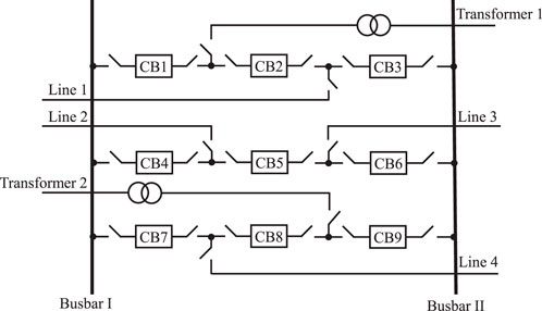
FIGURE 1. Breaker-and-a-half substation arrangement.

There are two busbars normally energized in the breaker-and-a-half arrangement. Three CBs in a bay are employed to electrically connect these two busbars, and a circuit exists between each two CBs. In this configuration, three CBs are utilized for two independent circuits and each circuit shares the same center CB. It is equivalent to a circuit with one and a half CBs (Council 2012). All CBs are activated in typical circumstances. Switching a line requires two CBs to be open. To switch line 1, for instance, CB2 and CB3 must be opened. While splitting busbars requires at least one CB in each bay to be open. For example, opening CB2, CB5, and CB8 at the same time can achieve the purpose of splitting the busbars. In this way, transformer 1, line 2, and line 4 are connected to busbar I, while transformer 2, line 1, and line 3 are connected to busbar II.

Based on the analysis mentioned above, a generalized substation model is created, as presented in Figure 2. Further, the mathematical model can be formulated based on the generalized substation model. In Figure 2, the generators, transmission lines, and loads can be connected to either busbar I or busbar II in each substation. Note that the connection positions of these components are determined by the introduced binary variables. The specific mathematical model will be introduced in Section 3.

FIGURE 2

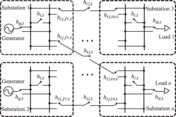
FIGURE 2. Generalized substation model.

3 Mathematical formulation

In this Section, a tri-level model is proposed as shown in Figure 3. The objective is to minimize the operation costs and load shedding/overgeneration penalty costs during transmission maintenance and under the worst-case scenario. The first level is to make TMS decisions and determines the network topology during the maintenance period, i.e., the status of transmission lines, and the connection positions of various components at each timestamp. In the second level, the damaged transmission lines that lead to the worst-case scenario are identified. Only the worst-case scenario is considered here since accurately predicting extreme weather events is usually not easy. It is acceptable to consider the worst-case situation when the specific disaster scenario is difficult to estimate. The third level is to re-dispatch generators to minimize the operation costs and load shedding/overgeneration penalty costs due to the failure of transmission lines in the second level.

FIGURE 3

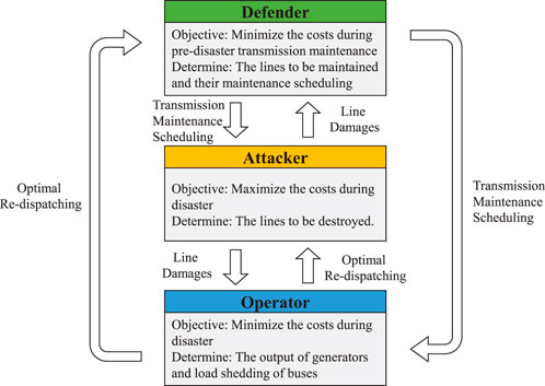
FIGURE 3. Framework of the proposed tri-level optimization model.

The overall proposed mathematical model is presented as follows.

The first-level problem is to make TMS decisions and determine the network topology, improving the economics during maintenance and mitigating the risk under the worst-case scenario, as presented in the objective function (1).

$\begin{array}{c}\underset{\mathit{x}\in \mathbb{X}}{\min }{C}^{pre}\left(\mathit{x}\right)+\mathrm{A}\mathrm{P}\left(\mathit{x}\right),\\ \mathrm{w}\mathrm{i}\mathrm{t}\mathrm{h}{C}^{pre}\left(\mathit{x}\right)={\displaystyle \sum }_{t\in T^{pre}}{\displaystyle \sum }_{g\in G}\left(c_g{P}_{g,t}^{pre}+c_g^{OG,pre}{\stackrel{\sim }{P}}_{g,t}^{pre}\right)+{\displaystyle \sum }_{t\in T^{pre}}{\displaystyle \sum }_{i\in I}{c}_i^{pre}{\stackrel{\sim }{P}}_{i,t}^{pre},\end{array}(1)$

where the superscript pre refers to pre-disaster, the same below, $c_g,c_g^{OG,pre},c_i^{pre}$ represent the marginal cost of generator g, the penalty cost for overgeneration of generator g, and load shedding of load connected to bus i, respectively, ${\stackrel{\sim }{P}}_{g,t}^{pre}$ and ${\stackrel{\sim }{P}}_{i,t}^{pre}$ represent the overgeneration of generator g at timestamp t, and load shedding of load connected to bus i, respectively.

Its feasible region can be summarized as $\mathit{X}=\left\{\left.\mathit{x}\right|\left(2\right)-\left(28\right),\forall t\in T^{pre}\right\}$:

There are mainly four maintenance scheduling constraints that should be considered (Marwali and Shahidehpour 1999; Liu et al., 2018; Zhang et al., 2022).

$x_{ij}\ge x_{ij,t},(2)$

${\displaystyle \sum }_{t\in T^{pre}}{x}_{ij,t}=T_{ij}^M,(3)$

$x_{ij,t+1}-x_{ij,t}\le x_{ij,t+\tau },\tau =\mathrm{2,3},...,T_{ij}^M,(4)$

${\displaystyle \sum }_{\left(i,j\right)\in L^M}{x}_{ij,t}\le X_t^{\max },(5)$

where $x_{ij}$ is a binary variable representing whether line (i, j) is maintained or not, 0 if not, otherwise 1, $x_{ij,t}$ is a binary variable representing the operating status of line (i, j) at timestamp t, 0 if line (i, j) works normally, otherwise 1, $T_{ij}^M$ represents the time required for maintenance of line (i, j), $L^M$ represents the set of defective transmission lines, $X_t^{\max }$ represents the maximum number of concurrent transmission maintenance at timestamp t.

Constraint (2) indicates the transmission lines only can be disconnected for maintenance. Constraint (3) states the time required for the maintenance of each transmission line. The continuity of maintenance is guaranteed by constraint (4). It indicates that maintenance activity can only stop when it is completed. Constraint (5) limites the number of lines that can be disconnected for maintenance at the same time.

$0\le P_{g,t,1}^{pre}\le P_g^{\max }\left(1-h_{g,t}\right),(6)$

$0\le P_{g,t,2}^{pre}\le P_g^{\max }{h}_{g,t},(7)$

$P_{g,t}^{pre}=P_{g,t,1}^{pre}+P_{g,t,2}^{pre},(8)$

$0\le {\stackrel{\sim }{P}}_{g,t,s}^{pre}\le P_{g,t,s}^{pre},(9)$

where $P_{g,t,s}^{pre}$ represents the power generation of generator g connected to busbar s (s = I or II) at timestamp t, $P_g^{\max }$ represents the power generation capability of generator g; $h_{g,t}$ is a binary variable representing the connection position of generator g at timestamp t, 0 if it is connected to busbar I, otherwise busbar II. Constraints (6), (7), and (8) determine the connection position, and power generation of the generator g. Constraint (9) limits the over-generation of each generator.

$P_{i,t,1}^{pre}=\left(1-h_{d,t}\right)P_{i,t}^{pre},(10)$

$P_{i,t,2}^{pre}=h_{d,t}{P}_{i,t}^{pre},(11)$

$0\le {\stackrel{\sim }{P}}_{d,t,s}^{pre}\le P_{d,t,s}^{pre},s=\mathrm{1,2},(12)$

${\stackrel{\sim }{P}}_{i,t}^{pre}={\stackrel{\sim }{P}}_{i,t,1}^{pre}+{\stackrel{\sim }{P}}_{i,t,2}^{pre},(13)$

where $P_{i,t,s}^{pre}$ represents the load connected to busbar s (s = I or II) of bus i at timestamp t, $P_{i,t}^{pre}$ represents the power demand of load connected to bus i; ${\stackrel{\sim }{P}}_{i,t,s}^{pre}$ represents the load shedding of load connected to busbar s (s = I or II) of bus i at timestamp t, ${\stackrel{\sim }{P}}_{i,t}^{pre}$ represents the load shedding of load connected to bus i at timestamp t, $h_{d,t}$ is a binary variable representing the connection position of load d at timestamp t, 0 if it is connected to busbar I, otherwise busbar II. Constraints (10) and (11) determine the connection position of loads. Constraint (12) and (13) limit the amount of load shedding.

$-\left(1-x_{ij,t}\right)\left(1-h_{ij,e,t}\right)P_{ij}^{\max }\le P_{ij,e,t,1}^{pre}\le \left(1-x_{ij,t}\right)\left(1-h_{ij,e,t}\right)P_{ij}^{\max },(14)$

$-\left(1-x_{ij,t}\right)h_{ij,e,t}{P}_{ij}^{\max }\le P_{ij,e,t,2}^{pre}\le \left(1-x_{ij,t}\right)h_{ij,e,t}{P}_{ij}^{\max },(15)$

$P_{ij,t}^{pre}=P_{ij,e,t,1}^{pre}+P_{ij,e,t,2}^{pre},\forall e,(16)$

where $P_{ij,t,s}^{pre}$ represents the power flow of line (i, j) connected to busbar s (s = I or II) at timestamp t, $P_{ij,e,t,s}^{pre}$ represents the power flow of line (i, j) whose end side e (e = i or j) connected to busbar s (s = I or II) at timestamp t, $P_{ij,t}^{pre}$ represents the power flow of line (i, j) at timestamp t, $P_{ij}^{\max }$ represents the rated capacity of transmission line (i, j), $h_{ij,e,t}$ is a binary variable representing the connection position of the end side e of line (i, j) at timestamp t, 0 if it is connected to busbar I, otherwise busbar II. Constraints (14) and (15) determine the connection position of both side of each transmission line. Constraint (16) determines the power flow through each transmission line.

$-h_{ij,e,t}{\theta }^M\le {\theta }_{ij,e,t}^{pre}-{\theta }_{ij,e,t,1}^{pre}\le h_{ij,e,t}{\theta }^M,(17)$

$-\left(1-h_{ij,e,t}\right){\theta }^M\le {\theta }_{ij,e,t}^{pre}-{\theta }_{ij,e,t,2}^{pre}\le \left(1-h_{ij,e,t}\right){\theta }^M,(18)$

$-M\left(1-h_{i,t}\right)\le {\theta }_{i,t,1}^{pre}-{\theta }_{i,t,2}^{pre}\le M\left(1-h_{i,t}\right),(19)$

where ${\theta }^M$ represents the maximum phase angle difference, ${\theta }_{ij,e,t}^{pre}$ represents the phase angle of end side e (e = i or j) of line (i, j) at timestamp t, ${\theta }_{ij,e,t,s}^{pre}$ represents the phase angle of line (i, j) whose end side e (e = i or j) connected to busbar s (s = I or II) at timestamp t. Constraints (17) and (18) indicate the phase angles of bus-bars are associated with the lines connected. Constraint (19) indicates the phase angles are not constrained when the busbar is splitting.

$P_{g,t}^{pre}-P_{g,t-1}^{pre}\le R_g^U,t\in T^{pre},(20)$

$P_{g,t-1}^{pre}-P_{g,t}^{pre}\le R_g^D,t\in T^{pre},(21)$

${\displaystyle \sum }_{g\in G_i}\left(P_{g,t,s}^{pre}-{\stackrel{\sim }{P}}_{g,t,s}^{pre}\right)-{\displaystyle \sum }_{\left(i,j\right)\in L{F}_i}{P}_{ij,t,s}^{pre}+{\displaystyle \sum }_{\left(i,j\right)\in L{T}_i}{P}_{ij,t,s}^{pre}=P_{i,t,s}-{\stackrel{\sim }{P}}_{i,t,s}^{pre},(22)$

$-M{x}_{ij,t}\le b_{ij}\left({\theta }_{i,t}^{pre}-{\theta }_{j,t}^{pre}\right)-P_{ij,t}^{pre}\le M{x}_{ij,t},(23)$

where $R_g^U$ and $R_g^D$ represent the ramp-up and ramp-down rates limit of generator g, respectively, $M$ is a sufficiently large constant, $b_{ij}$ is the susceptance of transmission line (i, j). ${\theta }_{i,t}^{pre}$ represents the phase angle of bus i at timestamp t. Constraints (20) and (21) limit the ramping up and down rates of each generator, respectively. Constraint (22) denotes the power balance should be guaranteed at each bus. Constraint (23) indicates the relationship between maintenance decision and power flow.

$h_{i,t}-1+h_{g,t}\le 0,(24)$

$h_{i,t}-1+h_{d,t}\le 0,(25)$

$h_{i,t}-1+h_{ij,e,t}\le 0,(26)$

${\displaystyle \sum }_{\left(i,j\right)\in L^M}{x}_{ij,t}+h_{i,t}\ge 1,(27)$

${\displaystyle \sum }_i\left(1-h_{i,t}\right)\le n,(28)$

where $h_{i,t}$ is a binary variable representing the state of busbar of bus i at timestamp t, 0 if bus-bar is splitting, otherwise 1. Constraints (24)–(26) indicate the generators, loads, and lines are forced to connect to Busbar 1 by default when no busbars are splitting. Constraint (27) indicates the busbars can only be split when the line is undergoing maintenance. Constraint (28) limits the number of busbars that can be split at the same time.

The second-level problem regards extreme weather events as attackers to power systems. It mainly involves choosing the transmission lines to destroy, which is related to the variables $x_{ij}$ at the first level. As shown in Eq. 29, the objective is to maximize the disruption, which is quantified by the operation costs and penalty costs after re-dispatching.

$\mathrm{A}\mathrm{P}\left(\mathit{x}\right)=\underset{\mathit{y}\in \mathbb{Y}}{\max }\mathrm{D}\mathrm{R}\mathrm{P}\left(\mathit{x},\mathit{y}\right),(29)$

Its feasible region can be summarized as $\mathit{Y}=\left\{\left.\mathit{y}\right|\left(30\right)-\left(33\right)\right\}$:

${\displaystyle \sum }_{\left(i,j\right)\in L}{S}_{ij}^1{y}_{ij}^1+{\displaystyle \sum }_{\left(i,j\right)\in L}{S}_{ij}^2{y}_{ij}^2\le Y,(30)$

$y_{ij}^0+y_{ij}^1+y_{ij}^2=1,(31)$

$y_{ij}^1=0,\forall \left(i,j\right)\in \left(L\backslash L^M\right),(32)$

$z_{ij}=y_{ij}^0+x_{ij}{y}_{ij}^1,(33)$

where $S_{ij}^1$ and $S_{ij}^2$ represent the attack resource consumption for damaging defective and normal lines, respectively, $y_{ij}^0$, $y_{ij}^1$ and $y_{ij}^2$ represent it will destroy line (i, j) in the way that the attack resource consumption is 0, $S_{ij}^1$; $S_{ij}^2$, respectively, Y is the total amount of preset attack resources, it is highly related to the weather severity; $z_{ij}$ represent the state of line (i, j) during disaster.

Constraint (30) limits the number of lines that can be attacked. Constraint (31) indicates that each line must be attacked in some way during extreme weather events. Here, different attack ways are classified according to the amount of attack resource consumption. It should be noted that if a line is attacked with an attack resource consumption of 0, it will continue to function normally. A defective line will fail while a normal line keeps working when the attack resource consumption is $S_{ij}^1$. If the attack resource consumption is $S_{ij}^2$, the line will be outage regardless of its condition. In the worst-case situation, attacking normal lines in the way that the attack resources consumption is $S_{ij}^1$ will not be performed because attacking in this way will only consume attack resources. Hence, constraint (32) guarantees that this attack way will not be executed on normal lines. Based on constraints (30)–(32), the ability of defective lines and normal lines to withstand extreme weather events can be distinguished. The transmission line status during extreme weather events is determined by constraint (33). If a defective line is maintained, it will not be destroyed easily during disasters. For example, when $x_{ij}=1$, it only fails when $y_{ij}^2=1$. Otherwise, the defective line only keeps normal when $y_{ij}^0=1$.

The response to the attack is formulated by the third-level optimization problem $\mathrm{D}\mathrm{R}\mathrm{P}\left(\mathit{x},\mathit{y}\right)$ in (34–47). Based on the decisions obtained in the first-level problem and the second-level problem, the power generation is re-scheduled to keep operation costs and penalty costs as low as possible.

$\begin{array}{c}\mathrm{D}\mathrm{R}\mathrm{P}\left(\mathit{x},\mathit{y}\right)=\underset{\mathit{p}\in \mathbb{P}\left(\mathit{x},\mathit{y}\right)}{\min }{C}^{dur}\left(\mathit{p}\right)\\ {\mathrm{w}\mathrm{i}\mathrm{t}\mathrm{h}C}^{dur}\left(\mathit{p}\right)={\displaystyle \sum }_{t\in T^{dur}}{\displaystyle \sum }_{g\in G}\left(c_g{P}_{g,t}^{dur}+c_g^{OG}{\stackrel{\sim }{P}}_{g,t}^{dur}\right)+{\displaystyle \sum }_{t\in T^{dur}}{\displaystyle \sum }_{i\in I}{c}_i^{dur}{\stackrel{\sim }{P}}_{i,t}^{dur},\end{array}(34)$

where the superscript dur refers to during disaster, the same below.

Its feasible region can be summarized as $=\left\{\left.\mathit{p}\right|\left(35\right)-\left(47\right)\right\}$ :

${\stackrel{\sim }{P}}_{i,t}^{dur}\ge 0,P_{g,t}^{dur}\ge 0,{\stackrel{\sim }{P}}_{g,t}^{dur}\ge 0,(35)$

$P_{i,t}-{\stackrel{\sim }{P}}_{i,t}^{dur}-{\displaystyle \sum }_{g\in G_i}\left(P_{g,t}^{dur}-{\stackrel{\sim }{P}}_{g,t}^{dur}\right)+{\displaystyle \sum }_{\left(i,j\right)\in L{F}_i}{P}_{ij,t}^{dur}-{\displaystyle \sum }_{\left(i,j\right)\in L{T}_i}{P}_{ij,t}^{dur}=0\left({\alpha }_{i,t}^1\right),(36)$

${\theta }_i^{\min }-{\theta }_{i,t}^{dur}\le 0\left({\alpha }_{i,t}^2\right),(37)$

${\theta }_{i,t}^{dur}-{\theta }_i^{\max }\le 0\left({\alpha }_{i,t}^3\right)(38)$

${\stackrel{\sim }{P}}_{i,t}^{dur}-P_{i,t}^{dur}\le 0\left({\alpha }_{i,t}^4\right),(39)$

$-b_{ij}\left({\theta }_{i,t}^{dur}-{\theta }_{j,t}^{dur}\right)+P_{ij,t}^{dur}-M\left(1-z_{ij}\right)\le 0\left({\beta }_{ij,t}^1\right),(40)$

$b_{ij}\left({\theta }_{i,t}^{dur}-{\theta }_{j,t}^{dur}\right)-P_{ij,t}^{dur}-M\left(1-z_{ij}\right)\le 0\left({\beta }_{ij,t}^2\right),(41)$

$-P_{ij}^{\max }{z}_{ij}-P_{ij,t}^{dur}\le 0\left({\beta }_{ij,t}^3\right),(42)$

$P_{ij,t}^{dur}-P_{ij}^{\max }{z}_{ij}\le 0\left({\beta }_{ij,t}^4\right),(43)$

$P_{g,t}^{dur}-P_g^{\max }\le 0\left({\gamma }_{g,t}^1\right),(44)$

$P_{g,t}^{dur}-P_{g,t-1}^{dur}-R_g^U\le 0\left({\gamma }_{g,t}^2\right),(45)$

$P_{g,t-1}^{dur}-P_{g,t}^{dur}-R_g^D\le 0\left({\gamma }_{g,t}^3\right),(46)$

${\stackrel{\sim }{P}}_{g,t}^{dur}-P_{g,t}^{dur}\le 0\left({\gamma }_{g,t}^4\right).(47)$

The parameters and variables in these formulas are similar to those in Eqs 6–28, but here they focus on power system operation during disasters. Hence, they will not be repeated here. Constraint (35) indicates that load shedding and power generation are non-negative. Constraint (36) ensures the power balance in each bus. Constraints (37) and (38) limit the size of the phase angle. Constraint (39) indicates the load shedding cannot exceed the load demand. Constraints (40) and (41) indicate the relationship between transmission line power flows and phase angles. Constraints (42) and (43) limit the amount of transmission line power flows. Constraints (44)–(46) denote the power generation of generators cannot exceed their technical limit, including the maximum generation, ramping up, and down rate. Constraint (47) restricts the amount of overgeneration of generators.

The non-linear constraints (14) and (15) resulting from the multiplications of two binary variables should be linearized. They can be linearized in a same way due to their similar structure. New binary variables need to be introduced. As an illustration, the linearization process of constraint (14) is presented as follows:

${\phi }_{l,e,t}^1\le 1-x_{l,t},(48)$

${\phi }_{l,e,t}^1\le 1-h_{l,e,t},(49)$

${\phi }_{l,e,t}^1\ge 1-x_{l,t}-h_{l,e,t},(50)$

$-{\phi }_{l,e,t}^1{P}_l^{\max }\le P_{l,e,t,1}^{pre}\le {\phi }_{l,e,t}^1{P}_l^{\max }.(51)$

4 Solution method

4.1 Problem reformulation

It is a popular method to utilize Karush-Kuhn-Tucker (KKT) conditions to transform the max-min problem into a single-level. In constraints (36)–(47), the variables enclosed in parenthesis at the end of each constraint are the dual variables corresponding to the constraints. Hence, the Lagrangian equation is written as follows:

$\begin{array}{l}\mathcal{L}={\displaystyle \sum }_{t\in T^{dur}}{\displaystyle \sum }_{g\in G}\left(c_g{P}_{g,t}^{dur}+c_g^{OG}{\stackrel{\sim }{P}}_{g,t}^{dur}\right)+{\displaystyle \sum }_{t\in T^{dur}}{\displaystyle \sum }_{i\in I}{c}_i^{dur}{\stackrel{\sim }{P}}_{i,t}^{dur}\\ +{\displaystyle \sum }_{t\in T^{dur}}{\displaystyle \sum }_{i\in I}{\alpha }_{i,t}^1\left(P_{i,t}^{dur}-{\stackrel{\sim }{P}}_{i,t}^{dur}-{\displaystyle \sum }_{g\in G_i}\left(P_{g,t}^{dur}-{\stackrel{\sim }{P}}_{g,t}^{dur}\right)+{\displaystyle \sum }_{\left(i,j\right)\in L{F}_i}{P}_{ij,t}^{dur}-{\displaystyle \sum }_{\left(i,j\right)\in L{T}_i}{P}_{ij,t}^{dur}\right)\\ +{\displaystyle \sum }_{t\in T^{dur}}{\displaystyle \sum }_{i\in I}{\alpha }_{i,t}^2\left({\theta }_i^{\min }-{\theta }_{i,t}^{dur}\right)\\ +{\displaystyle \sum }_{t\in T^{dur}}{\displaystyle \sum }_{i\in I}{\alpha }_{i,t}^3\left({\theta }_{i,t}^{dur}-{\theta }_i^{\max }\right)\\ +{\displaystyle \sum }_{t\in T^{dur}}{\displaystyle \sum }_{i\in I}{\alpha }_{i,t}^4\left({\stackrel{\sim }{P}}_{i,t}^{dur}-P_{i,t}^{dur}\right)\\ +{\displaystyle \sum }_{t\in T^{dur}}{\displaystyle \sum }_{\left(i,j\right)\in L}{\beta }_{ij,t}^1\left(-b_{ij}\left({\theta }_{i,t}^{dur}-{\theta }_{j,t}^{dur}\right)+P_{ij,t}^{dur}-M\left(1-z_{ij}\right)\right)\\ +{\displaystyle \sum }_{t\in T^{dur}}{\displaystyle \sum }_{\left(i,j\right)\in L}{\beta }_{ij,t}^2\left(b_{ij}\left({\theta }_{i,t}^{dur}-{\theta }_{j,t}^{dur}\right)-P_{ij,t}^{dur}-M\left(1-z_{ij}\right)\right)\\ +{\displaystyle \sum }_{t\in T^{dur}}{\displaystyle \sum }_{\left(i,j\right)\in L}{\beta }_{ij,t}^3\left(-P_{ij}^{\max }{z}_{ij}-P_{ij,t}^{dur}\right)\\ +{\displaystyle \sum }_{t\in T^{dur}}{\displaystyle \sum }_{\left(i,j\right)\in L}{\beta }_{ij,t}^4\left(P_{ij,t}^{dur}-P_{ij}^{\max }{z}_{ij}\right)\\ +{\displaystyle \sum }_{t\in T^{dur}}{\displaystyle \sum }_{g\in G}{\gamma }_{g,t}^1\left(P_{g,t}^{dur}-P_g^{\max }\right)\\ +{\displaystyle \sum }_{t\in T^{dur}}{\displaystyle \sum }_{g\in G}{\gamma }_{g,t}^2\left(P_{g,t}^{dur}-P_{g,t-1}^{dur}-R_g^U\right)\\ +{\displaystyle \sum }_{t\in T^{dur}}{\displaystyle \sum }_{g\in G}{\gamma }_{g,t}^3\left(P_{g,t-1}^{dur}-P_{g,t}^{dur}-R_g^D\right)\\ +{\displaystyle \sum }_{t\in T^{dur}}{\displaystyle \sum }_{g\in G}{\gamma }_{g,t}^4\left({\stackrel{\sim }{P}}_{g,t}^{dur}-P_{g,t}^{dur}\right)\end{array}(52)$

whose optimality occurs at

$\frac{\partial \mathcal{L}}{\partial {\stackrel{\sim }{P}}_{i,t}^{dur}}=c_i^{dur}-{\alpha }_{i,t}^1+{\alpha }_{i,t}^4\ge 0,(53)$

$\frac{\partial \mathcal{L}}{\partial P_{g,t}^{dur}}=c_g-{\alpha }_{i,t}^1+{\gamma }_{g,t}^1+{\gamma }_{g,t}^2-{\gamma }_{g,t+1}^2+{\gamma }_{g,t+1}^3-{\gamma }_{g,t}^3-{\gamma }_{g,t}^4\ge 0,(54)$

$\frac{\partial \mathcal{L}}{\partial {\stackrel{\sim }{P}}_{g,t}^{dur}}=c_g^{OG}+{\alpha }_{i,t}^1+{\gamma }_{g,t}^4\ge 0,(55)$

$\frac{\partial \mathcal{L}}{\partial {\theta }_{i,t}^{dur}}=-{\alpha }_{i,t}^2+{\alpha }_{i,t}^3+{\displaystyle \sum }_{\left(i,j\right)\in L\left(i,\cdot \right)}{b}_{ij}\left({\beta }_{ij,t}^2-{\beta }_{ij,t}^1\right)+{\displaystyle \sum }_{\left(i,j\right)\in L\left(\cdot ,i\right)}{b}_{ij}\left({\beta }_{ij,t}^1-{\beta }_{ij,t}^2\right)=0,(56)$

$\frac{\partial \mathcal{L}}{\partial P_{ij,t}^{dur}}={\alpha }_{i,t}^1-{\alpha }_{j,t}^1+{\beta }_{ij,t}^1-{\beta }_{ij,t}^2-{\beta }_{ij,t}^3+{\beta }_{ij,t}^4=0,(57)$

${\alpha }_{i,t}^{1}free,a_{i,t}^2,{\alpha }_{i,t}^3,{\alpha }_{i,t}^4\ge 0,{\beta }_{ij,t}^1,{\beta }_{ij,t}^2,{\beta }_{ij,t}^3,{\beta }_{ij,t}^4\ge 0,{\gamma }_{g,t}^1,{\gamma }_{g,t}^2,{\gamma }_{g,t}^3,{\gamma }_{g,t}^4\ge 0.(58)$

By using the optimality condition, we can reformulate original max-min problem as follows.

$\begin{array}{l}\underset{\mathit{y}\in \mathit{Y}}{\max }\underset{\mathit{p}\in \mathit{P}}{\min }{\displaystyle \sum }_{t\in T^{dur}}{\displaystyle \sum }_{g\in G}{c}_g{P}_{g,t}^{dur}+{\displaystyle \sum }_{t\in T^{dur}}{\displaystyle \sum }_{i\in I}{c}_i^{dur}{\stackrel{\sim }{P}}_{i,t}^{dur}\\ =\max {\displaystyle \sum }_{t\in T^{dur}}{\displaystyle \sum }_{i\in I}\left({\alpha }_{i,t}^1{P}_{i,t}^{dur}+{\alpha }_{i,t}^2{\theta }_i^{\min }-{\alpha }_{i,t}^3{\theta }_i^{\max }-{\alpha }_{i,t}^4{P}_{i,t}^{dur}\right)\\ -{\displaystyle \sum }_{t\in T^{dur}}{\displaystyle \sum }_{\left(i,j\right)\in L}\left(M\left(1-z_{ij}\right)\left({\beta }_{ij,t}^1+{\beta }_{ij,t}^2\right)+P_{ij}^{\max }{z}_{ij}\left({\beta }_{ij,t}^3+{\beta }_{ij,t}^4\right)\right)\\ -{\displaystyle \sum }_{t\in T^{dur}}{\displaystyle \sum }_{g\in G}\left({\gamma }_{g,t}^1{P}_g^{\max }+{\gamma }_{g,t}^2{R}_g^U+{\gamma }_{g,t}^3{R}_g^D\right)\end{array},(59)$

s.t. (30)–(33), (53)–(58).

There are bilinear terms in the objective function (59). We replace $M\left(1-z_{ij}\right){\beta }_{ij,t}^1$ with ${\lambda }_{ij,t}^1$, and introduce the following two additional constraints.

$\left\{\begin{array}{cc}{\lambda }_{ij,t}^1\ge M{\beta }_{ij,t}^1-M{z}_{ij}& \forall \left(i,j\right)\in L,\\ {\lambda }_{ij,t}^1\ge 0& \forall \left(i,j\right)\in L,\end{array}\right.(60)$

Similarly, $M\left(1-y_{ij}\right){\beta }_{ij,t}^2$ is replaced with ${\lambda }_{ij,t}^2$.

$\left\{\begin{array}{cc}{\lambda }_{ij,t}^2\ge M{\beta }_{ij,t}^2-M{z}_{ij}& \forall \left(i,j\right)\in L,\\ {\lambda }_{ij,t}^2\ge 0& \forall \left(i,j\right)\in L,\end{array}\right.(61)$

We replace $y_{ij}{\beta }_{ij,t}^3$ with ${\lambda }_{ij,t}^3$.

$\left\{\begin{array}{cc}{\lambda }_{ij,t}^3\ge {\beta }_{ij,t}^3-M\left(1-z_{ij}\right)& \forall \left(i,j\right)\in L,\\ {\lambda }_{ij,t}^3\ge 0& \forall \left(i,j\right)\in L,\end{array}\right.(62)$

Similarly, $y_{ij}{\beta }_{ij,t}^4$ is replaced with ${\lambda }_{ij,t}^4$.

$\left\{\begin{array}{cc}{\lambda }_{ij,t}^4\ge {\beta }_{ij,t}^4-M\left(1-z_{ij}\right)& \forall \left(i,j\right)\in L,\\ {\lambda }_{ij,t}^4\ge 0& \forall \left(i,j\right)\in L,\end{array}\right.(63)$

Therefore, the objective function (59) can be further modified as follows.

$\begin{array}{l}\max {\displaystyle \sum }_{t\in T^{dur}}{\displaystyle \sum }_{i\in I}\left({\alpha }_{i,t}^1{P}_{i,t}^{dur}+{\alpha }_{i,t}^2{\theta }_i^{\min }-{\alpha }_{i,t}^3{\theta }_i^{\max }-{\alpha }_{i,t}^4{P}_{i,t}^{dur}\right)\\ -{\displaystyle \sum }_{t\in T^{dur}}{\displaystyle \sum }_{\left(i,j\right)\in L}\left(\left({\lambda }_{ij,t}^1+{\lambda }_{ij,t}^2\right)+P_{ij}^{\max }\left({\lambda }_{ij,t}^3+{\lambda }_{ij,t}^4\right)\right)\\ -{\displaystyle \sum }_{t\in T^{dur}}{\displaystyle \sum }_{g\in G}\left({\gamma }_{g,t}^1{P}_g^{\max }+{\gamma }_{g,t}^2{R}_g^U+{\gamma }_{g,t}^3{R}_g^D\right)\end{array}.(64)$

In this way, the proposed tri-level optimization model is reformulated as a bi-level optimization model.

4.2 Solution algorithm

The bi-level optimization model can be further decoupled into a master problem and a subproblem. The master problem selects the defective transmission lines and schedules their maintenance. The subproblem identifies the line failures that result in the maximum operation costs. The C&CG algorithm is a common-used method to solve the bi-level robust optimization. The main principle of C&CG algorithm is to repeatedly add the worst damage scenarios from subproblem and relevant variables to the master problem in each iteration until the optimal solution is obtained. To illustrate the detailed steps of the C&CG algorithm, the compact notation of the master problem considering the worst damage scenarios $\widehat{\mathbb{Y}}=\left\{{\widehat{\mathit{y}}}^k,k=1,...,m\right\}$ can be written as follows.

$\underset{\mathit{x}\in \mathbb{X},{\mathit{p}}^s\in \mathbb{P}\left(\mathit{x},{\widehat{\mathit{y}}}^s\right)}{\min }{C}^{pre}\left(\mathit{x}\right)+\xi .(65)$

subject to

$\xi \ge C^{dur}\left({\mathit{p}}^k\right),\forall k\in 1,...,m,(66)$

${\mathit{A}\mathit{p}}^k+\mathit{B}\mathit{x}+\mathit{D}{\widehat{\mathit{y}}}^k\le \mathit{E},(67)$

where $\mathit{A}$, $\mathit{B}$, $\mathit{D}$, and $\mathit{E}$ are coefficient matrices used to describe constraints (35)–(47). $\xi$ is a scalar variable introduced to guarantee that the master problem dominates the included worst damage scenarios.

Solving the master problem based on a set of scenarios obtained by the subproblem can yield maintenance decision ${\mathit{x}}^k$ and a lower bound (LB) of the original optimization model. Based on ${\mathit{x}}^k$, the subproblem described in (64) subjecting to constraints (30)–(33) (53)–(58), and (60)–(63) can be solved which determines the worst damage scenario. Further, the optimal value of the subproblem plus the operation costs during transmission maintenance of the corresponding maintenance decision ${\mathit{x}}^k$ gets an upper bound (UB) of the original optimization model. An optimal solution can be obtained by performing the aforementioned steps repeatedly until the difference between the UB and LB is less than the predefined optimality gap.

The key steps of the C&CG algorithm are outlined in Algorithm 1. Note that the master problem is solved assuming all the lines work in the first iteration.

Algorithm 1. The C&CG algorithm

Step 1: Initialization: Set all lines in operation, LB = − ∞, UB = ∞, k = 1, and optimality gap ε = 10⁻⁶.

Step 2: Master Problem Optimization: Solve master problem and get the first-level optimal solution x^k and LB = $C^{pre}\left({\mathit{x}}^k\right)$ + ξ^k.

Step 3: Subproblem Optimization: Solve subproblem for the current maintenance decision x^k to obtain the worst-case damage scenario y^k and UB = min{UB, $C^{pre}\left({\mathit{x}}^k\right)+C^{dur}\left({\mathit{p}}^k\right)$}.

Step 4: Termination: If $\mathrm{U}\mathrm{B}-\mathrm{L}\mathrm{B}\le \epsilon$, stop. Current x^k is the optimal transmission maintenance scheduling. Otherwise, k = k + 1, add constraints corresponding to the new worst damage scenario to master problem and go to Step 2.

5 Case study

In this section, numerical experiments are carried out to demonstrate the effectiveness of the proposed method. The proposed MILP model is established with YALMIP toolbox (Lofberg 2004) and solved by Gurobi solver in Matlab.

5.1 Test system and data

The modified IEEE RTS-79 system (Subcommittee 1979) is employed as the test system. The load data of the 28th week is utilized. The rated capacities of lines 25, 26, and 27 are restricted to 0.35 p. u. The capacities of the remaining branches are limited to 0.6 p. u. Assume that the busbars at buses 9 and 21 have the ability to split. The penalty costs for overgeneration and load shedding in the maintenance period are both set at 200$/MWh and those during disasters are both set at 500$/MWh (Du et al., 2018). The former is lower than the latter because the overgeneration and load shedding in the maintenance period are planned, and the impact on power users is relatively light. The defective transmission lines are presented in Table 1. Additionally, destroying a defective line requires 1 attack resource, and destroying a normal line requires 2 attack resources, that is $S_{ij}^1=1$, and $S_{ij}^2=2$. The marginal costs of generators can be found in (Nemati et al., 2018). Finally, the period of preventive maintenance is assumed to be 3 days, and the disaster time is assumed to be 1 day.

TABLE 1

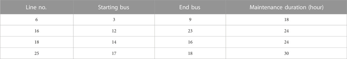
TABLE 1. Maintenance data of defective transmission lines.

5.2 Calculation result

The following instances are studied to investigate the effectiveness of the proposed method. The uncertainty budget Y in all cases is set to be 5.

Case 1: Do not consider maintaining any defective transmission lines.

Case 2: Only TMS is considered.

Case 3: NTO can be utilized during transmission maintenance. Note that NTO can only be employed when the transmission line is maintained.

The lines 6, 16, 18 and 25 are selected for maintenance in both Case 2 and Case 3. However, there is a difference between the scheduled maintenance periods in the two cases, as listed in Table 2.

TABLE 2

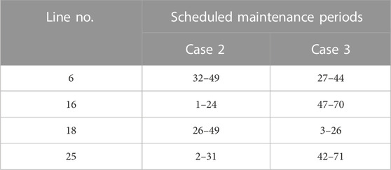
TABLE 2. Scheduled transmission maintenance periods in case 2 and case 3.

The in-disaster and pre-disaster costs of the three cases are presented in Figure 4. According to the results, Case 1 has the greatest in-disaster cost, whereas Case 2 and Case 3 have the same in-disaster cost. Case 1 does not maintain any defective transmission lines, leading to more lines will be destroyed under the set uncertainty budget. Specifically, if lines 6, 16, 17, and 18 are destroyed together in the disaster, it would incur an in-disaster cost of $3.0547 million in Case 1. But in Case 2 and in Case 3, all defective lines are selected for maintenance, and the worst case will happen when lines 5, and 9 are interrupted. In this situation, the in-disaster cost is only $1.4899 million. The results show the effectiveness of pre-disaster transmission maintenance in disaster prevention.

FIGURE 4

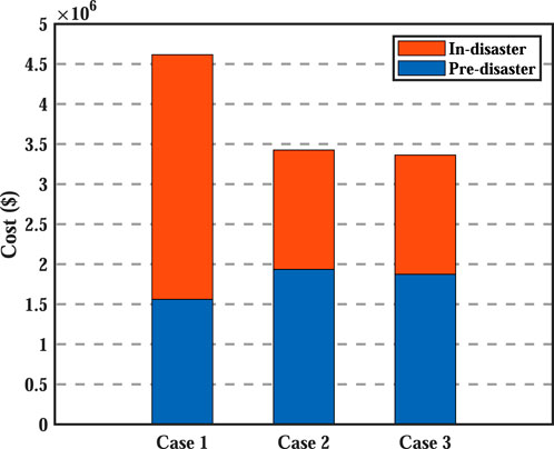
FIGURE 4. Calculation results of three cases.

Furthermore, the pre-disaster operation cost increase in Case 2 and Case 3 compared to Case 1 can be regarded as the cost of taking preventive measures against disasters. It can be found that the pre-disaster operation cost increased by 24.02% from $1.5609 million in Case 1 to $1.9359 million in Case 2. However, the cost increment is reduced by 16.62% if NTO is considered during transmission maintenance. The discrepancy between the pre-disaster operation costs of Case 2 and Case 3 can be regarded as the benefits of utilizing NTO. In other words, NTO can significantly reduce the cost increase due to transmission maintenance.

5.3 Analysis of the effect of NTO

To explore the effect of NTO, we set up a controlled numerical experiment, called Case 4. In this case, the scheduled maintenance period setting is the same as that of Case 3 but NTO is not considered during the period. The total cost of Case 4 is $3.4623 million, which is a little higher than that of Case 2. Further, we define the branch utilization rate ${\mu }_{ij,t}$ as the ratio of the power flow on the branch (i, j) to the rated capacity of the branch at timestamp t, the specific calculation is presented as Eq. 68. Finally, the utilization rate of each branch of Case 3 and Case 4 when line 18 is under maintenance is presented using the form of the heat map in Figure 5. Figure 5A shows the situation without NTO, while Figure 5B is the opposite.

${\mu }_{ij,t}=\left|\frac{P_{ij,t}}{P_{ij}^{\max }}\right|\times 100\%.(68)$

FIGURE 5

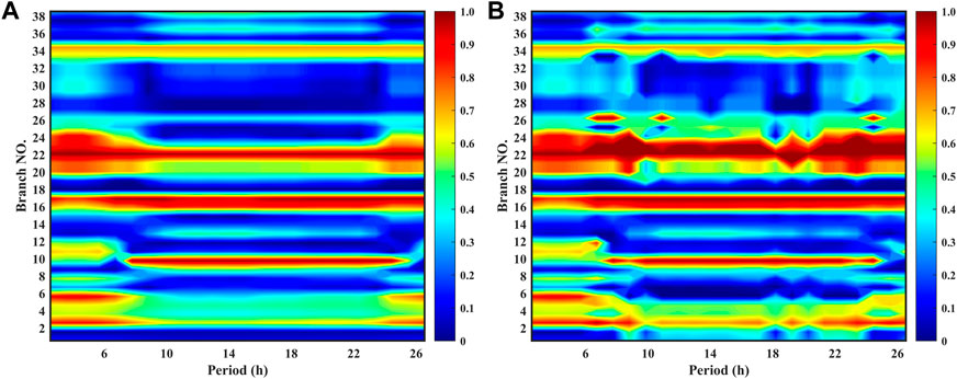
FIGURE 5. The utilization of each branch during scheduling maintenance periods 3–26 h. (A) Without NTO, (B) with NTO.

It can be seen that the distribution of power flow is adjusted through NTO. Compared to Case 4, some transmission lines in Case 3 have higher utilization rates. For instance, the utilization rate of lines 20–26 has changed significantly. Generators located on buses 18, 21, and 22 cost relatively less than other generators, and lines 20, 21, 25, and 26 are important lines that transmit power from these generators. Hence, the increased utilization of these lines can be helpful to decrease operation costs. The results indicate that NTO can effectively improve the power system economics during maintenance.

5.4 Analysis of the uncertainty budget

To investigate the impact of weather severity on the maintenance plan based on the proposed model, we conduct experiments with different uncertainty attack budgets that are highly related to weather intensity. Table 3 shows the pre-disaster cost with maintenance, in-disaster cost with and without maintenance, and scheduled line for maintenance under different attack budgets.

TABLE 3

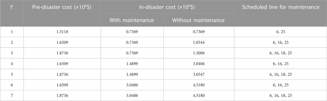
TABLE 3. The results under different attack budgets.

Generally, pre-disaster transmission maintenance is always advantageous. Note that, such a benefit is modest when the attack budget Y is low. It can be noticed that the in-disaster costs are the same with and without maintenance when Y equals 1. In this situation, the worst case occurs when line 18 is destroyed. However, if line 18 is selected for maintenance, the increase in pre-disaster cost will be slightly greater than the reduction in in-disaster cost, making it likely not an optimal decision. When lines 6 and 25 are selected for maintenance, the pre-disaster cost does not increase but decreases. It also shows the positive effect of NTO on transmission maintenance.

As Y increases, the gain of pre-disaster transmission maintenance becomes more significant. Noteworthy, for the cases of Y = 6 and Y = 7, although the worst-case scenarios are different, the resulting in-disaster costs are the same. However, it does not mean that the maintenance plans of these two cases will be the same. As a comparison, we set the maintenance plan in the case of Y = 7 to the maintenance plan in the case of Y = 6, and the in-disaster cost at this time is equal to the in-disaster cost without maintenance. This makes the maintenance of other defective lines less meaningful.

To sum up, the decision-makers should select an appropriate maintenance plan to achieve their desired trade-off between cost and benefit. On the other hand, the maintenance plan is highly correlated with the value of the attack budget. Therefore, it is necessary to predict the weather intensity as accurately as possible to make the value of Y more reasonable. Otherwise, we cannot properly derive an effective maintenance plan.

6 Conclusion

This paper proposes an innovative model to schedule transmission maintenance against extreme weather events. A tri-level optimization model is established to comprehensively consider the economics of pre-disaster transmission maintenance and power system resilience during a disaster. The first level is to make TMS decision and determine the transmission network topology during maintenance. The second level is to select the transmission lines whose outages will result in the worst scenarios. The third level is to re-dispatch the power generation to minimize operation costs in the worst scenarios. The modified IEEE RTS-79 system is used for case studies. The following are the findings from the case studies.

1) Appropriate pre-disaster transmission maintenance can effectively enhance power system resilience, thereby reducing load shedding during extreme weather events.

2) The optimization of network topology during the maintenance period can adjust the power flow and consequently improve power system economics during transmission maintenance.

3) The maintenance plan is significantly associated with the value of the attack budget. It means that an effective maintenance plan is based on accurate prediction of extreme weather events.

Data availability statement

The raw data supporting the conclusion of this article will be made available by the authors, without undue reservation.

Author contributions

WZ: Conceptualization, Methodology, Software, Validation, Formal analysis, Investigation, Data curation, Original draft, Writing, review and editing. CS: Conceptualization, Supervision, Writing, review and editing. BH: Conceptualization, Funding acquisition, Supervision, Writing, review and editing. KX: Conceptualization, Supervision, Writing, review and editing.

Funding

This work was supported by the National Natural Science Foundation of China under Grant 52022016.

Conflict of interest

The authors declare that the research was conducted in the absence of any commercial or financial relationships that could be construed as a potential conflict of interest.

Publisher’s note

All claims expressed in this article are solely those of the authors and do not necessarily represent those of their affiliated organizations, or those of the publisher, the editors and the reviewers. Any product that may be evaluated in this article, or claim that may be made by its manufacturer, is not guaranteed or endorsed by the publisher.

References

Council National Research, (2012). Terrorism and the electric power delivery system. Washington, D.C., USA, National Academies Press doi:10.17226/12050

CrossRef Full Text | Google Scholar

Du, E., Zhang, N., Kang, C., and Xia, Q. (2018). Scenario map based stochastic unit commitment. IEEE Trans. Power Syst. 33 (5), 4694–4705. doi:10.1109/TPWRS.2018.2799954

CrossRef Full Text | Google Scholar

Fisher, E. B., O’Neill, R. P., and Ferris, M. C. (2008). Optimal transmission switching. IEEE Trans. Power Syst. 23 (3), 1346–1355. doi:10.1109/TPWRS.2008.922256

CrossRef Full Text | Google Scholar

Ganganath, Nuwan, Wang, Jing V., Xu, Xinzhi, Cheng, Chi-Tsun, and Tse, Chi K. (2018). Agglomerative clustering-based network partitioning for parallel power system restoration. IEEE Trans. Industrial Inf. 14 (8), 3325–3333. doi:10.1109/TII.2017.2780167

CrossRef Full Text | Google Scholar

Gao, Haixiang, Chen, Ying, Mei, Shengwei, Huang, Shaowei, and Xu, Yin (2017). Resilience-oriented pre-hurricane resource allocation in distribution systems considering electric buses. Proc. IEEE 105 (7), 1214–1233. doi:10.1109/JPROC.2017.2666548

CrossRef Full Text | Google Scholar

Heidarifar, Majid, and Ghasemi, Hassan (2016). A network topology optimization model based on substation and node-breaker modeling. IEEE Trans. Power Syst. 31 (1), 247–255. doi:10.1109/TPWRS.2015.2399473

CrossRef Full Text | Google Scholar

Hosseini, Mohammad Mehdi, and Parvania, Masood (2022). Resilient operation of distribution grids using deep reinforcement learning. IEEE Trans. Industrial Inf. 18 (3), 2100–2109. doi:10.1109/TII.2021.3086080

CrossRef Full Text | Google Scholar

Huang, Gang, Wang, Jianhui, Chen, Chen, Qi, Junjian, and Guo, Chuangxin (2017). Integration of preventive and emergency responses for power grid resilience enhancement. IEEE Trans. Power Syst. 32 (6), 4451–4463. doi:10.1109/TPWRS.2017.2685640

CrossRef Full Text | Google Scholar

Jamborsalamati, Pouya, Hossain, M. J., Taghizadeh, Seyedfoad, Konstantinou, Georgios, Manbachi, Moein, and Dehghanian, Payman (2020). Enhancing power grid resilience through an iec61850-based EV-assisted load restoration. IEEE Trans. Industrial Inf. 16 (3), 1799–1810. doi:10.1109/TII.2019.2923714

CrossRef Full Text | Google Scholar

Lei, Shunbo, Wang, Jianhui, Chen, Chen, and Hou, Yunhe (2018). Mobile emergency generator pre-positioning and real-time allocation for resilient response to natural disasters. IEEE Trans. Smart Grid 9 (3), 1–41. doi:10.1109/TSG.2016.2605692

CrossRef Full Text | Google Scholar

Li, Yanlin, Xie, Kaigui, Wang, Lingfeng, and Xiang, Yingmeng (2019). Exploiting network topology optimization and demand side management to improve bulk power system resilience under windstorms. Electr. Power Syst. Res. 171 (June), 127–140. doi:10.1016/j.epsr.2019.02.014

CrossRef Full Text | Google Scholar

Liu, J., Kazemi, M., Motamedi, A., Zareipour, H., and Rippon, J. (2018). Security-constrained optimal scheduling of transmission outages with load curtailment. IEEE Trans. Power Syst. 33 (1), 921–931. doi:10.1109/TPWRS.2017.2694424

CrossRef Full Text | Google Scholar

Lofberg, J. (September 2004). Yalmip: A toolbox for modeling and optimization in matlab, Proceedings of the IEEE international conference on robotics and automation (IEEE cat. No.04CH37508). Taipei Taiwan: IEEE, 284–289. doi:10.1109/CACSD.2004.1393890

CrossRef Full Text | Google Scholar

Mahzarnia, Maedeh, Parsa Moghaddam, Mohsen, Payam Teimourzadeh Baboli, , and Siano, Pierluigi (2020). A review of the measures to enhance power systems resilience. IEEE Syst. J. 14 (3), 4059–4070. doi:10.1109/JSYST.2020.2965993

CrossRef Full Text | Google Scholar

Marwali, M. K. C., and Shahidehpour, S. M. (May 1999). Short-term transmission line maintenance scheduling in a deregulated system, Proceedings of the 21st International Conference on Power Industry Computer Applications. Connecting Utilities. PICA 99. To the Millennium and Beyond (Cat. No.99CH36351), 31–37. Santa Clara CA USA: IEEE, doi:10.1109/PICA.1999.779382

CrossRef Full Text | Google Scholar

Moradi-Sepahvand, Mojtaba, Amraee, Turaj, and Gougheri, Saleh Sadeghi (2022). Deep learning based hurricane resilient coplanning of transmission lines, battery energy storages, and wind farms. IEEE Trans. Industrial Inf. 18 (3), 2120–2131. doi:10.1109/TII.2021.3074397

CrossRef Full Text | Google Scholar

Nemati, Hadi, Latify, Mohammad Amin, and Reza Yousefi, G. (2018). Coordinated generation and transmission expansion planning for a power system under physical deliberate attacks. Int. J. Electr. Power & Energy Syst. 96 (March), 208–221. doi:10.1016/j.ijepes.2017.09.031

CrossRef Full Text | Google Scholar

Noaa National Centers for Environmental Information (Ncei) U.S (2021). Billion-dollar weather and climate disasters. Available at: https://www.ncdc.noaa.gov/billions/.

Google Scholar

Panteli, Mathaios, Trakas, Dimitris N., Mancarella, Pierluigi, and Hatziargyriou, Nikos D. (2016). Boosting the power grid resilience to extreme weather events using defensive islanding. IEEE Trans. Smart Grid 7 (6), 2913–2922. doi:10.1109/TSG.2016.2535228

CrossRef Full Text | Google Scholar

Stanković, A. M., Tomsovic, K. L., De Caro, F., Braun, M., Chow, J. H., Äukalevski, N., et al. (2022). Methods for analysis and quantification of power system resilience. IEEE Trans. Power Syst., 1–14. Force, IEEE PES Task. doi:10.1109/TPWRS.2022.3212688

CrossRef Full Text | Google Scholar

Subcommittee, Probability (1979). IEEE reliability test system. IEEE Trans. Power Apparatus Syst. PAS- 98 (6), 2047–2054. doi:10.1109/TPAS.1979.319398

CrossRef Full Text | Google Scholar

Sun, Lei, Lin, Zhenzhi, Xu, Yan, Wen, Fushuan, Zhang, Can, and Xue, Yusheng (2019). Optimal skeleton-network restoration considering generator start-up sequence and load pickup. IEEE Trans. Smart Grid 10 (3), 3174–3185. doi:10.1109/TSG.2018.2820012

CrossRef Full Text | Google Scholar

Sun, Wei, Liu, Chen-Ching, and Zhang, Li (2011). Optimal generator start-up strategy for bulk power system restoration. IEEE Trans. Power Syst. 26 (3), 1357–1366. doi:10.1109/TPWRS.2010.2089646

CrossRef Full Text | Google Scholar

Wang, Chong, Hou, Yunhe, Qiu, Feng, Lei, Shunbo, and Liu, Kai (2017). Resilience enhancement with sequentially proactive operation strategies. IEEE Trans. Power Syst. 32 (4), 2847–2857. doi:10.1109/TPWRS.2016.2622858

CrossRef Full Text | Google Scholar

Xiang, Yuwei, Wang, Tong, and Wang, Zengping (2022). Risk prediction based preventive islanding scheme for power system under typhoon involved with rainstorm events. IEEE Trans. Power Syst., 1–14. doi:10.1109/TPWRS.2022.3219519

CrossRef Full Text | Google Scholar

Yan, Jiahao, Hu, Bo, Shao, Changzheng, Huang, Wei, Sun, Yue, Zhang, Weixin, et al. (2022). Scheduling post-disaster power system repair with incomplete failure information: A learning-to-rank approach. IEEE Trans. Power Syst. 1, 4630–4641. –1. doi:10.1109/TPWRS.2022.3149983

CrossRef Full Text | Google Scholar

Zeng, Bo, and Zhao, Long (2013). Solving two-stage robust optimization problems using a column-and-constraint generation method. Operations Res. Lett. 41 (5), 457–461. doi:10.1016/j.orl.2013.05.003

CrossRef Full Text | Google Scholar

Zhang, Weixin, Hu, Bo, Xie, Kaigui, Shao, Changzheng, Niu, Tao, Yan, Jiahao, et al. (2022). Short-term transmission maintenance scheduling considering network topology optimization. J. Mod. Power Syst. Clean Energy 10 (4), 883–893. doi:10.35833/MPCE.2020.000937

CrossRef Full Text | Google Scholar

Zhang, Weixin, Shao, Changzheng, Hu, Bo, Xie, Kaigui, Siano, Pierluigi, Li, Mushui, et al. (2022a). Transmission defense hardening against typhoon disasters under decision-dependent uncertainty. IEEE Trans. Power Syst., 1–11. doi:10.1109/TPWRS.2022.3194307

CrossRef Full Text | Google Scholar

Zhang, Weixin, Shao, Changzheng, Hu, Bo, Zhou, Jiahao, Cao, Maosen, Xie, Kaigui, et al. (2022b). Proactive security-constrained unit commitment against typhoon disasters: An approximate dynamic programming approach. IEEE Trans. Industrial Inf., 1–10. doi:10.1109/TII.2022.3208574

CrossRef Full Text | Google Scholar