Numerical study on the mechanism of fluid energy transfer in an axial flow pump impeller under the rotating coordinate system

It is a necessary condition to obtain the fluid movement law and energy transfer and loss mechanism in the impeller of the axial pump for achieving an efficient and accurate design of the axial flow pump. Based on the shear stress transport k-ω turbulence model, a three-dimensional unsteady numerical simulation of the whole flow field of an axial flow pump was presented at different flow rates. Combined with the Bernoulli equation of relative motion, the flow field structure in the impeller under design condition was studied quantitatively in the rotating coordinate system. The fluid movement law and energy transfer and loss mechanism in the impeller of the axial flow pump was described in detail. In the relative coordinate system, the mechanical energy of the fluid on the same flow surface conserves. The dynamic energy is continuously transformed into pressure energy from the leading edge to the trailing edge and the dynamic energy is continuously transformed into pressure energy from the leading edge to the trailing edge. The energy conversion is mainly completed in the front half of the blade. The friction loss and the mixing loss are the basic sources of losses in the impeller flow passage. Most hydraulic losses of impeller flow passage are caused by friction and the hydraulic losses near the trailing edge are dominated by mixing loss. This research has certain reference significance for further understanding the flow field structure in the impeller of the axial flow pump, improving its design theory and method, and then realizing its efficient and accurate design of the axial flow pump.

1 Introduction

The deteriorating climate has made energy conservation and emission reduction a common goal of all countries in the world. Climatologists pointed out that only if the emissions of greenhouse gas must be close to the peak by 2025 at the latest and reduce by 43% before 2050, can the earth’s temperature rise be controlled by 1.5°C (Skea, et al., 2022). As one of three subtypes of blade pumps that consume 10% of global power generation each year, the others being mixed flow pump and centrifugal pump, axial flow pumps, also known as propeller pumps, are used in applications requiring very high flow rates and low pressures, such as long-distance water transfer, flood dewatering, and irrigation systems and pumped storage. Improving the efficiency of the axial flow pump is very important for achieving the carbon peak. However, mastering the movement law and energy transfer and loss mechanism of the fluid in the axial flow pump, especially in the impeller is the premise to improve the efficiency of axial flow pump.

In 1755, the Swiss mathematician Euler first proposed the constitutive equation of ideal fluid motion (Euler equation). It gave the law of fluid energy transfer in the pump theoretically and provided a theoretical basis for the design of blade pumps for the first time, but could not explain the cause of fluid energy loss in the pump. In 1785, John Skeys applied for and registered the structural patent of the axial flow pump, which is the earliest prototype of the axial flow pump in the world; In 1850, British scientist James Thomson installed guide vanes at the downstream of the impeller to improve the efficiency of the axial flow pump; In 1875, British scientist Osborne Reynolds designed the front guide vane for the axial flow pump for the first time, which further improved the efficiency of axial flow pump; In 1904, Prandtl put forward the boundary layer theory creatively, which was the first time to combine theoretical fluid mechanics and engineering fluid mechanics closely. It is a milestone in the history of fluid mechanics and fluid machinery. The boundary layer theory provided a theoretical basis for explaining the cause of fluid energy loss in the axial flow pump (Lazarkiewicz.and Troskolanski, 1965).

The boundary layer theory was applied rapidly to the study of the mechanism of fluid energy loss in the axial flow pumps. Generally speaking, hydraulic losses in the axial flow pump include inlet passage loss, impeller loss, guide vane loss and outlet pipe loss. The loss of the inlet and outlet channels is proportional to the square of the absolute velocity at the corresponding position. The loss of the axial flow pump impeller and guide vane is mainly in two forms: airfoil loss (blade surface friction loss and wake mixing loss) and non-airfoil loss due to limited wingspan (secondary flow loss in impeller channel and leakage loss due to the tip clearance). Professor Staritzky et al. (Srinivasan, 1966; Staritski, 1958; Staritski, 1964; Stefanovski, 1940) believed that the non-airfoil loss at the design operating point could be negligible compared with the airfoil loss (it accounted for about 5% of the total loss), and relevant tests also confirmed this argument (Csanady, 1964).

Some scholars tried to calculate the airfoil loss through the thickness of the boundary layer (Loitsanski, 1959; Srinivasan, 1968; Mac-Gregor, 1952; Markoff, 1948; Stepanoff, 1962; Proscura, 1954; Schlichting, 1979), and they gave the calculation methods of airfoil loss in several cascade systems. Some methods only considered the airfoil loss in the cascade, while some methods also considered the loss caused by wake mixing; Among them, the calculation method of Professor Loitsanski, (Proscura, 1954; Schlichting, 1979) is more accurate than other calculation methods.

Since the 21st century, CFD has been gradually applied in various industrial fields including the axial flow pump. It makes a big difference in studying the flow field structure of the axial flow pump such as cavitation (Wang, et al., 2021), tip leakage flow (Shen, et al., 2021; Zhang, et al., 2012), and pressure fluctuation (Shen, et al., 2019; F. Yang, et al., 2022). At the same time, it makes it possible to carry out quantitative research on the mechanism of flow loss in pumps. (Kan, et al., 2022) investigated the influences of the tip leakage vortex on the axial flow pump as turbine through numerical simulations, where the energy loss mechanism due to tip leakage flow was revealed K. (Pu, et al., 2022) studied the influence of vortex on steady flow and pressure fluctuation of circulating axial pump through numerical simulations, where energy loss caused by the low-speed vortex was analyzed quantitatively and the structure position of the low-speed vortex can be predicted Li et al. (Li, et al., 2021) studied the energy loss mechanism of a mixed-flow pump under stall condition with the numerical method. Especially, the combination of entropy generation theory and numerical simulation can well conduct quantitative research on the hydraulic loss of the pump (Zhou, et al., 2022; Xin, et al., 2022; Li, et al., 2020; Cui and Zhang, 2020) in recent years, which can describe the proportion of hydraulic loss of each flow passage component of the pump under different working conditions.

The Bernoulli equation of relative motion has given the mechanism of the energy transfer from the impeller inlet to the outlet in the view of theory. An unsteady numerical simulation of the whole flow field of an axial flow pump was carried out in this study based on the SST k- ω turbulence model. Combined with the Bernoulli equation of the relative motion and the numerical calculation results of the flow field structure in the impeller, the mechanism of energy transfer and loss in the impeller was revealed, which could provide a certain reference for the enrichment of the design theory of the axial flow pump.

2 Research project and method

2.1 Pump model

An axial flow pump with a design volume flow rate of 0.35 m³/s, head of 6.7m, and rotation speed of 1450 rpm was chosen as the research object. The 3D model of the axial flow pump is shown in Figure 1. The whole pump section consists of five flow passage parts, namely the suction chamber, impeller, guide vane, support, and pressurized chamber. In addition, the diameter of pump impeller is 300 mm, the hub ratio is 0.5, the tip clearance is 0.2 mm, the impeller has four blades and the guide vane has seven blades.

FIGURE 1

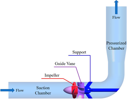
FIGURE 1. Axial flow pump model.

2.2 Governing equations

Three governing equations, mass conservation equation, momentum conservation equation, and energy conservation equation, dominate the motion in the axial flow pump. For a general axial flow pump, its working pressure is low and the amplitude of the temperature change is small, so the density of the fluid medium could be considered constant and the heat transfer can be ignored. Eqs. 1, 2 show the tensor forms of the mass conservation equation and momentum conservation equation of the viscous incompressible medium.

$\frac{\partial u_i}{\partial x_i}=0(1)$

$\frac{\partial u_i}{\partial \mathit{t}}+u_j\frac{\partial u_i}{\partial x_j}=F_i-\frac{1}{\rho }\frac{\partial p}{\partial x_i}+\upsilon \frac{{\partial }^2{u}_i}{\partial x_j\partial x_j}(2)$

where,

$u_i$ is the velocity component in the x, y, and z directions

$F_i$ is the mass force

$p$ is the pressure

$\rho$ is the medium density

$\upsilon$ is the medium kinematic viscosity.

SST k- ω turbulence model was selected for this study, which can predict effectively the fluid separation point under the condition of reverse pressure. At the same time, when solving the low Reynolds number flow near the wall area, the SST k- ω turbulence model has higher accuracy. Its basic equations are as follows:

$\frac{\partial \left(\rho k\right)}{\partial t}+\frac{\partial \left(\rho u_{j}k\right)}{\partial x_j}=\frac{\partial }{\partial x_j}\left[\left(\mu +\frac{{\mu }_t}{{\sigma }_k}\right)\frac{\partial k}{\partial x_j}\right]+{\tau }_{ij}\frac{\partial u_i}{\partial x_j}-{\beta }^{*}\rho \omega k(3)$

$\frac{\partial \left(\rho \omega \right)}{\partial t}+\frac{\partial \left(\rho u_j\omega \right)}{\partial x_j}=\frac{\partial }{\partial x_j}\left[\left(\mu +\frac{{\mu }_t}{{\sigma }_{\omega }}\right)\frac{\partial k}{\partial x_j}\right]+\frac{\gamma }{{\nu }_t}{\tau }_{ij}\frac{\partial u_i}{\partial x_j}-\beta \rho {\omega }^2+2\left(1-F_1\right)\rho {\sigma }_{{\omega }^2}\frac{1}{\omega }\frac{\partial k}{\partial x_j}\frac{\partial \omega }{\partial x_j}(4)$

where, ${\sigma }_k$=1.176, ${\sigma }_{\omega }$=2, $\beta$=0.075, ${\beta }^{*}$=0.09, $\kappa$=0.41, ${\gamma }_1=\beta /{\beta }^{*}-{\sigma }_{\omega }{\kappa }^2/\sqrt{{\beta }^{*}}$.

$F_1=\tanh \left({\arg }_1^4\right)(5)$

${\arg }_1=\min \left(\max \left(\frac{\sqrt{k}}{{\beta }^{*}\omega y};\frac{500\nu }{y^2\omega }\right);\frac{4\rho k}{CD{\sigma }_{\omega 2}{y}^2}\right)(6)$

$CD=\max \left(2\rho \frac{1}{{\sigma }_{\omega 2}\omega }\frac{\partial k}{\partial x_j}\frac{\partial \omega }{\partial x_j},1.0\times {10}^{-10}\right)(7)$

where, F₁ is a mixed function. F₁ = 1 in the area near the wall, which means that the whole area uses the k- ω turbulence model, and F₁ = 0 in the area far always from the wall, which means that the whole area uses the standard k- ε turbulence model, $y$ is the distance from the first layer of the grid to the wall, ${\sigma }_{\omega 2}$= 1.168. The limiting equation of eddy viscosity is as follows:

$v_t=\frac{a_{1}k}{\max \left(a_1\omega ,S{F}_2\right)}(8)$

$v_t={\mu }_t/\rho (9)$

where, ${\mu }_t$ is turbulent viscosity, S is an invariant measure of strain rate, F₂ is also a mixed function, which is equal to 1 in the boundary layer and 0 in the shear layer, and $a_1$ is a constant, equal to 5/9.

$\begin{array}{l}{F}_2=\tanh \left({\arg }_2^2\right)\\ {\arg }_2=\max \left\{2\frac{\sqrt{k}}{0.09\omega y};\frac{500\nu }{y^2\omega }\right\}\end{array}(10)$

2.3 Computational setup

As a kind of low Reynolds number turbulence model, the SST k-ω turbulence model requires that $y+\le 1$, which will ensure that at least one layer of grid exists within the viscous sublayer. However, it is a requirement that is almost impossible to meet unless a large number of grids that ordinary servers cannot afford are adopted. It has been shown in relevant research (Tao, 2001)that the first layer of the grid near the wall will also fall in the viscous sublayer when $y+\le 5$. The $y+$ near the wall of the impeller and guide vane is shown in Figure 2, where all the $y+$ near the blades is small than five and the final average of $y+$ is 1.1, and the growth rate of the grids off the wall is 1.1.

FIGURE 2

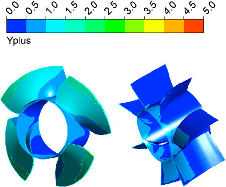
FIGURE 2. The y + distribution of grids near the wall.

All the flow passage components of the axial flow pump were meshed by hexahedral structured grids. The grid independence was judged by the change of pump efficiency with the increasing of the number of grids. When the efficiency change amplitude did not exceed 2% with the increase of the number of grids, it could be considered that the grid independence verification was passed, which was shown in Figure 3. In addition, the grid independence verification was carried out under the condition that $y+$ meets the requirements of the SST k-ω turbulence model. The final grids of the computing domain verified by grid independence were shown Table. 1 and Figure 4.

FIGURE 3

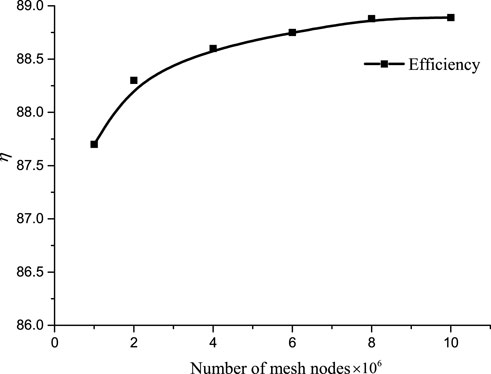
FIGURE 3. Results of grid independence.

TABLE 1

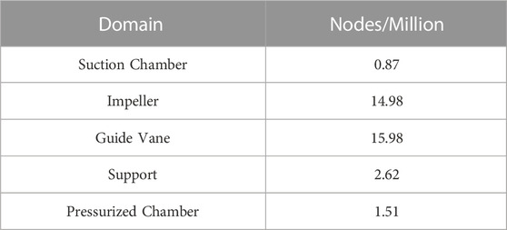
TABLE 1. Mesh details for each domain.

FIGURE 4

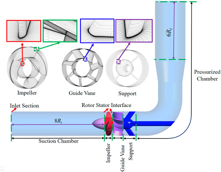
FIGURE 4. Flow domains and grids.

The whole numerical calculation was completed by ANSYS-CFX 20.1 The medium is water with a density of 998.2 kg/m³ and a dynamic viscosity of 0.000889 Pas. The rotating speed of the impeller was set to 1450rpm and all the other flow passages were stationary. A mass flow boundary (350 kg/s) with a turbulent intensity of 5% was adopted at the inlet of the computational domain and a pressure boundary (1 atm) was set at the outlet of the computational domain. All walls were subject to non-slip-wall boundary condition. Since the accuracy of the unsteady calculation results is higher than that of the steady calculation results, the unsteady calculation results were used in this study. However, the unsteady calculation requires the steady calculation results as the initial condition to accelerate convergence. The interfaces between the rotating region and the stationary region adopted the interface of the frozen rotor in the steady calculation, while the sliding grids were used in the unsteady calculation. The time-step size was set as 0.000115 s, which is the time for the rotor to turn for one degree to obtain sufficient flow field solution accuracy (Lin, et al., 2021). By changing the flow rate at the inlet boundary of the computational domain, the numerical calculation of the flow field structure in the axial flow pump under different flow rate conditions was completed. In addition, to weaken the influence of the inlet and outlet boundary conditions on the calculation results of the flow field in the axial flow pump, it is necessary to keep a sufficient distance between the inlet and outlet boundary and the axial flow pump. The distance between the inlet of the suction chamber and the impeller inlet was set as 8 R_t, and the distance between the end of the diffusion section and the outlet of the pressurized chamber was set as 6 R_t.

2.4 Numerical calculation accuracy verification

In order to verify the accuracy of numerical simulation, we completed the external characteristic test of the axial flow pump on the closed test bench. The schematic diagram of the test bench is shown in Figure 5 and the experimental instruments are shown in Figure 6, in which the uncertainty of the flowmeter is lower than 1.5%, the speed uncertainty of the torque speed sensor is less than 0.2% and the torque uncertainty of that is less than 1.5%, and the uncertainty of the pressure sensors is less than 1%. The external characteristic test at different flow rate was completed by adjusting the regulating valve opening. All the data were converted to digital form and stored in a computer database.

FIGURE 5

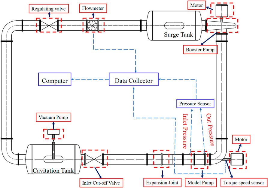
FIGURE 5. Schematic map of the hydraulic test rig.

FIGURE 6

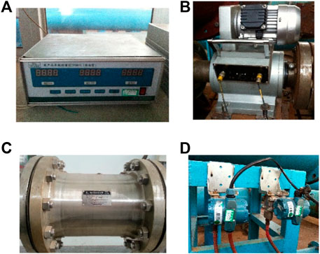
FIGURE 6. Measuring instruments: (A) data collector, (B) torque speed sensor, (C) flowmeter and (D) pressure sensor.

The numerical calculation results of the external characteristic curves, the head, and efficiency, of the axial flow pump were compared with the test results as shown in Figure 7. The simulation results are in good agreement with the test results near the design mass flowrate (0.35 m³/s) condition. However, when the deviation from the design mass flow rate condition is too large, there is an obvious difference between the test value and the CFD value. Especially under the condition of small flow rate, the difference between the test results and the CFD results is the most obvious, which has lost reference value to the engineering practice. So, the turbulence model SST k-ω has sufficient accuracy in predicting the flow field structure under the design mass flow rate condition of the axial flow pump.

FIGURE 7

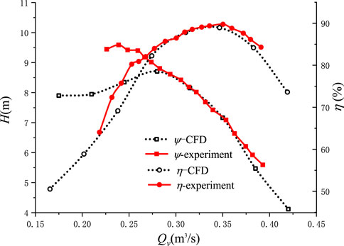
FIGURE 7. External characteristic analysis.

3 Results and discussion

3.1 Energy transfer mechanism in the impeller of the axial-flow pump

As we know, in the circumferential direction of specific axial and radial coefficient positions, the pressure, velocity, liquid flow angle, and other physical parameters in the impeller passage of the axial flow pump are periodically and symmetrically distributed. However, only the average value in space is taken as the design value in the design process of the axial flow pump. It also has been confirmed that the average value of the impeller inlet flow field structure in space is in good agreement with the theoretical design value under the design condition (Guo, et al., 2022) which proved that it is feasible to study the energy transfer and loss mechanism in the impeller passage using the weighted average treatment of the flow field structure in the impeller passage. The energy transfer and loss mechanism in the axial flow pump impeller was studied by using the method of the weighted average of mass flow rate in the circumferential direction in this study.

$x_{MCA}=\frac{\sum \left(\Delta m\cdot x\right)}{m}(11)$

where x is the physical variable, $x_{MCA}$ is the weighted average value of x in the circumferential direction based on the mass flow rate at the position of the specific streamwise location and radius coefficient. So, the weighted average value based on the mass flow of the parameters at different streamwise locations and different radius coefficients could be studied on the meridional surface. The data processing diagram is shown in Figure 8.

FIGURE 8

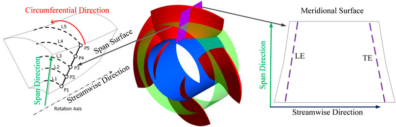
FIGURE 8. The diagram of the weighted average of parameters based on mass flow.

Equation 11 is the Bernoulli equation for the ideal fluid in the relative coordinate system. For a horizontal axial flow pump, the impeller inlet height is as same as the outlet center height, namely, $z_1=z_2$. And so are the diameter of the impeller inlet and outlet. Then the circumferential velocity is the same, that is, Eq. 11 is transformed into Eq. 12, from which, it could be deduced that fluid maintains conservation of the mechanical energy from the impeller inlet to the outlet in the relative coordinate system and the dynamic energy is continuously transformed into the pressure energy.

$z_1+\frac{p_{1-t}}{\rho g}+\frac{V_{1-re}^2-U_1^2}{2g}=z_2+\frac{p_{2-t}}{\rho g}+\frac{V_{2-re}^2-U_2^2}{2g}(12)$

$\frac{p_{1-t}}{\rho g}+\frac{V_{1-re}^2}{2g}=\frac{p_{2-t}}{\rho g}+\frac{V_{2-re}^2}{2g}(13)$

The pressure coefficients are defined as follows to represent visually the energy change at the impeller inlet to a higher degree.

$C_p=\frac{p-\overline{p_{\text{in}}}}{0.5\rho V_{in}^2},C_d=\frac{0.5\rho V^2}{0.5\rho V_{in}^2},C_{tot}=C_p+C_d(14)$

where, $\overline{p_{in}}$ is the average pressure at the pump inlet, $C_p$ is the static pressure coefficient, $C_d$ is the dynamic pressure coefficient, $C_{tot}$ is the total pressure coefficient.

The flow surface of radius 0.5 was taken as the research object. The energy coefficients on the flow surface were processed by weighted average based on the mass flow. Equation 12 is changed into Eq. 13.

$C_{1t-tot-rel-MCA}=C_{2t-tot-rel-MCA}(15)$

$C_{1t-p-MCA}+C_{1-d-rel-MCA}=C_{2t-p-MCA}+C_{2-d-rel-MCA}(16)$

$C_{1-tot-rel-MCA}=C_{2-tot-rel-MCA}+∆C_{\left(1-2\right)-tot-rel-MCA}(17)$

The coefficients are defined as follows to represent the energy change visually in the impeller passage to a higher degree.

$C_p=\frac{p-p_{\text{in}}}{0.5\rho V_{in-re}^2},C_d=\frac{0.5\rho V_{re}^2}{0.5\rho V_{in}^2},C_{tot}=C_p+C_d(18)$

where,

$p_{\text{in}}$ is the pressure at the pump inlet

$V_{in-re}$ is the relative velocity at the pump inlet

$C_p$ is the pressure coefficient

$C_d$ is the dynamic pressure coefficient

$C_{tot}$ is the total pressure coefficient.

As shown in Figure 9, the total pressure coefficient in the relative coordinate system decreases slowly from the impeller inlet to the outlet and the decreasing range is very small, which proves the correctness of the theoretical analysis. That is, the mechanical energy of the fluid on the same flow surface in the impeller channel is conserved. The reason why the total pressure coefficient decreases slowly from the impeller inlet to the outlet is the hydraulic loss caused by the viscosity as shown in Eq. 15. The hydraulic loss consists of the friction loss caused by friction and the mixed loss caused by the boundary layer separation. The dynamic energy is constantly converted into pressure energy from the impeller inlet to the outlet as a whole in the relative coordinate system, which is the source of the pressure head of the axial flow pump.

FIGURE 9

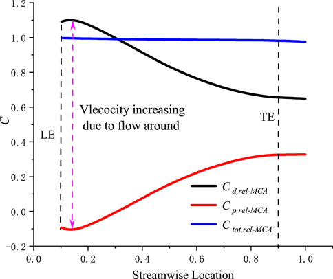
FIGURE 9. The distribution curve of the weighted average of the energy head coefficient based on the mass flow on the flow surface of R* = 0.5.

However, it is easy to be noticed that the fluid dynamic pressure coefficient increases slightly before decreasing rapidly. On a specific flow surface of the impeller passage, it can be regarded as an infinite plane cascade. The aerodynamic theory has pointed out that a high speed and low pressure region will appear at the suction surface of the airfoil near the leading edge due to flow around the airfoil, so is the cascade in the impeller passage as shown in Figure 11C.

The theoretical head of the pump is defined as the sum of the dynamic head and the theoretical static head in the absolute coordinate system, in which, the theoretical static head is the difference between the theoretical pressure head from the impeller outlet to the inlet (Eq. 17), and the dynamic head is the difference of the velocity head in the absolute coordinate system between the impeller outlet and the inlet (Eq. 18). According to the relative Bernoulli equation, the theoretical pressure head difference between the impeller outlet and the inlet is equal to the velocity head difference between the impeller inlet and the outlet in the relative coordinate system, as shown in Eq. 17. The inlet and outlet velocity triangles of the impeller are shown in Figure 10. From the impeller inlet to outlet, the relative velocity gradually decreases and the dynamic energy is converted into the pressure energy. The reverse pressure gradient always exists in the whole impeller channel. The reverse pressure gradient will increase the thickness of the boundary layer and then, lead to its separation, which will cause great mixing loss. It is also the fundamental reason why the efficiency of the axial flow pump is lower than that of the axial flow turbine.

$H_t=H_{P-t}+H_d(19)$

$H_{p-t}=\frac{p_{2-t}}{\rho g}-\frac{p_{1-t}}{\rho g}=\frac{V_{1-re}^2}{2g}-\frac{V_{2-re}^2}{2g}(20)$

$H_d=\frac{V_{2-stn}^2-V_{1-stn}^2}{2g}(21)$

FIGURE 10

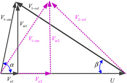
FIGURE 10. The velocity triangle at the impeller inlet and outlet.

According to the velocity triangle, the relative velocity can be expressed as Eq. 19.

$V_{re}^2=V_m^2+{\left(U-V_u\right)}^2(22)$

The normal inlet is always adopted in the design of the axial flow pump, that is, $V_{u1}$ = 0 m/s and the impeller inlet and outlet of the axial flow pump have the same diameter, that is, $V_{m1}=V_{m2}$ and $U_1=U_2$ , The theoretical static head Eq. 22 can be derived from Eqs. 20, 21.

$V_{1-re}^2=V_{m1}^2+{\left(U_1-V_{u1}\right)}^2=V_{m1}^2+U_1^2(23)$

$V_{2-re}^2=V_{m2}^2+{\left(U_2-V_{u2}\right)}^2=V_{m2}^2+U_2^2+V_{u2}^2-2U_2{V}_{u2}(24)$

$H_{p-t}=\frac{2U_2{V}_{u2}-V_{u2}^2}{2g}(25)$

Equation 23 could be derived from the further derivation of Eq. 17.

$H_d=\frac{V_{u2}^2}{2g}(26)$

The dynamic head is completely determined by the circumferential velocity component at the impeller outlet. Equation 24 is the theoretical head expression for the axial flow pump.

$H_t=\frac{U_2{V}_{u2}}{g}(27)$

The actual head of the impeller could be calculated by Eqs. 25, 26. The theoretical head can also be expressed by Eq. 27. The actual head must be less than the theoretical head due to the hydraulic loss. It is not difficult to find out that the actual head and the theoretical head have the same dynamic head by comparing Eqs. 26, 27. The difference between them mainly exists in the static head. It has been described that the total energy in the relative coordinate system will decrease slowly because of the hydraulic loss in Eq. 15. The dynamic energy in the relative coordinate system could not be completely converted into the pressure energy without any hydraulic loss. During the flow process, the dynamic energy must be partially converted into internal energy in the form of friction and mixing caused by boundary layer separation, and then lost. The hydraulic loss is equal to the relative total energy reduction.

$H=H_p+H_d(28)$

$H=\frac{p_2}{\rho g}-\frac{p_1}{\rho g}+\frac{V_{2-stn}^2}{2g}-\frac{V_{1-stn}^2}{2g}=\frac{p_2}{\rho g}-\frac{p_1}{\rho g}+\frac{V_{u2}^2}{2g}(29)$

$H_t=\frac{p_{2-t}}{\rho g}-\frac{p_{1-t}}{\rho g}+\frac{V_{u2}^2}{2g}=\frac{V_{1-rel}^2-V_{1-rel}^2}{2g}+\frac{V_{u2}^2}{2g}(30)$

3.2 Energy transfer mechanism in the impeller of the axial-flow pump

The weighted average value of the performance characteristics such as H_d, H_p, H, H_t and $\Delta C_{tot-rel}$ on the flow surface of R* 0.5 based on mass flow were taken as shown in Figure 11A and were recorded as H_d-MCA, H_p-MCA, H_MCA, H_t-MCA and $\Delta C_{tot-rel-MCA}$ ($\Delta C_{tot-rel-MCA}$ = H_t-MCA- H_MCA).

FIGURE 11

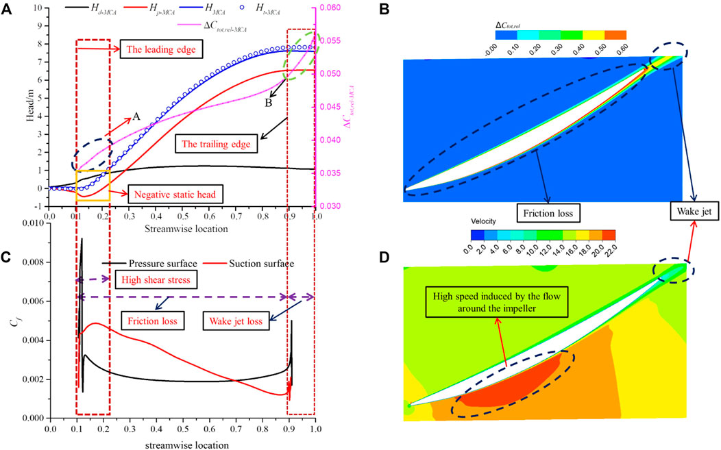
FIGURE 11. The energy transfer and loss mechanism on the surface of R* = 0.5: (A) The distribution curve of the coefficients of the head and relative total pressure loss with the flow direction coefficient; (B) The distribution curve of the friction coefficient; (C) The relative total pressure loss coefficient contour; (D) The relative velocity contour.

The static head is the main part of the axial flow pump head. It is mainly obtained by converting the relative dynamic energy into the pressure energy and the transformation is completed in the front half of the blade. The static head shows a trend of decreasing at first and then increasing on the whole flow surface, which is consistent with the changing trend of the static pressure coefficient in Figure 9. The negative static head exists near the leading edge, which is caused by that the flow around the blade will increase the relative velocity of the flow field near the leading edge of the suction surface (Figure 11D). This area is also the place most prone to cavitation. For the axial flow pump with a specific size, the key to improving its cavitation performance is to control the relative velocity at the suction surface of the leading edge. The dynamic head increases rapidly at the leading edge of the blade and then tends to be flat. It is also obtained mainly in the front half of the blade.

It is not difficult to infer that the actual head of the impeller is also mainly obtained in the front half flow passage. From the perspective of energy transmission, the torque formed by the pressure difference between the pressure surface and the suction surface is the fundamental source of the fluid energy. As shown in Figure 12, the pressure coefficient increases slowly from the leading edge to the trailing edge, while the pressure coefficient of the suction surface decreases rapidly near the leading edge and then up to be the same as that of the trailing edge gradually. The negative pressure coefficient at the front half of the whole blade is maintained on the suction surface of the blade. Therefore, the pressure difference between the pressure surface and the suction surface at the front half of the blade is far larger than that at the second half of the blade, which means that the torque on the front half of the blade is far larger than that on the second half. That is the reason why the actual head of the impeller is mainly obtained in the front half flow passage.

FIGURE 12

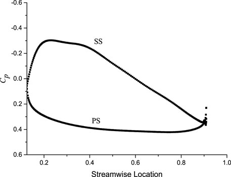
FIGURE 12. The distribution of the pressure coefficient on the blade surface at the radial coefficient of 0.5.

The friction loss caused by the velocity gradient in the boundary layer and the mixing loss caused by the separation of the boundary layer is the basic source of losses in the impeller flow passage. It can be seen from the distribution of the relative total pressure loss coefficient from the impeller inlet to the impeller outlet in Figure 11A that the gradient of the relative total pressure loss coefficient near the leading edge (Area A) and the trailing edge (Area B) is larger than that in the area between them, while the gradient near the trailing edge is greater than that near the leading edge. The relative velocity of the fluid near the leading edge at the suction surface of the blade will increase significantly due to the flow around the blade, which will result in a corresponding increase in the friction shear stress coefficient at this location as shown in Figure 11B. The greater the shear stress coefficient, the greater the friction loss gradient. Then, as the relative velocity decreases, the shear stress coefficient decreases, and the gradient of the relative total pressure loss coefficient decreases. The impeller passage of the axial flow pump, as we know, is basically under the adverse pressure gradient, and the adverse pressure gradient at the suction surface is obvious larger than that at the pressure surface. The thickness of the boundary layer on the suction surface increases gradually under the action of the adverse pressure gradient and reaches the maximum at the trailing edge as shown in Figure 11D. For the turbulent boundary layer, there is violent mixing movement in its interior. The thicker the boundary layer, the more mixing loss and therefore it can be seen that the relative total pressure loss coefficient gradient increases significantly at the trailing edge. In addition, the wake jet is formed after the fluid leaves the blade and it will result in more severe mixing loss. The gradient of the relative total pressure loss coefficient will also further increase.

Overall, on the one hand, friction loss is the main form of hydraulic loss in most areas of the impeller flow passage except the trailing edge, and the gradient of the relative total pressure loss coefficient is obviously greater because of the flow around the blade. On the other hand, the mixing loss inside the boundary layer and wake is the main form of hydraulic loss at the trailing edge. The gradient of the relative total pressure loss coefficient caused by mixing loss in the wake is the largest in the whole impeller flow passage. The point to improve pump efficiency is to avoid boundary layer separation in the flow channel and to eliminate the wake as soon as possible to prevent it from spreading in the downstream channel.

Figure 13 shows the distribution of the weighted average value of H_t, H and $\eta$ based on the mass flow on the meridional surface of the impeller flow passage. The trend of the theoretical head (Figure 13A) and the actual head (Figure 13B) in the main flow area (Radial coefficient between 0.05 and 0.95) are basically consistent. They gradually increase from the impeller inlet to the outlet and the impeller has high hydraulic efficiency. However, the circumferential velocity component, $V_u$, of the fluid near the hub (Radial coefficient between 0 and 0.05) is large due to the rotation of the hub. According to the Euler equation, the increase of the circumferential velocity component means the increase of the theoretical head. The rotation of the blade tip makes the fluid near the rim (Radial coefficient between 0.95 and 1) maintain a high circumferential velocity component, while the flange wall makes the axial velocity in the tip area attenuate rapidly. Therefore, the absolute velocity of the fluid in this area is dominated by the circumferential direction. According to the Euler equation, this area will have a high theoretical head.

FIGURE 13

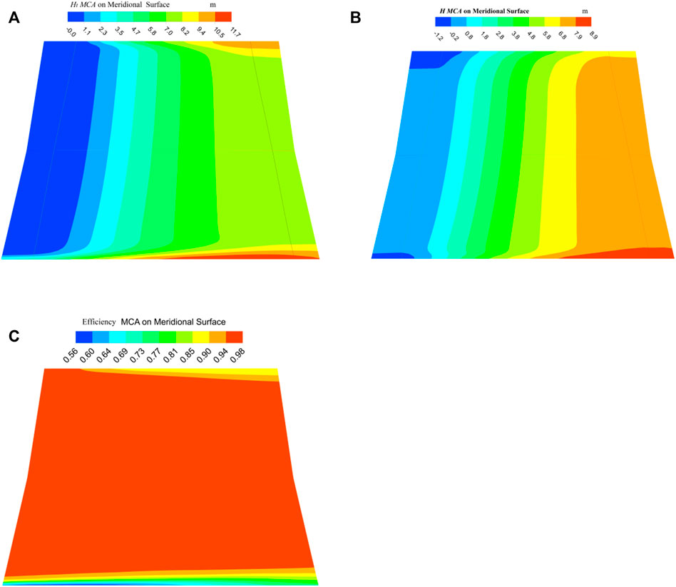
FIGURE 13. The contour of the weighted average of the head and efficiency coefficients based on mass flow: (A) The theoretical head; (B) The head; (C) The efficiency.

The actual head is the difference between the theoretical head and the hydraulic loss head. The fluid in the pressure surface will return to the suction surface of the blade through the clearance between the tip and the rim under the effect of the pressure difference between the pressure surface and the suction surface, which is called tip leakage flow. The tip leakage flow will cause complex leakage vortex, which will damage the flow field structure at the rim seriously and cause a lot of hydraulic loss. As a result, the actual head in this area also decreases. The actual head in the rim is obviously lower than that in other locations with the same streamwise location as shown in Figure 13B.

Efficiency is the ratio of the actual head to the theoretical head as shown in Figure 13C. It has been analyzed that the fluid in the main flow area has higher hydraulic efficiency because of that the main losses in this area are caused by the friction loss of the airfoil surface and the wake mixing loss of the trailing edge, which are small, while the hydraulic efficiency drops rapidly near the hub and rim. The fluid near the hub area is mainly affected by the corner separation, that near the rim area is mainly affected by the leakage vortex.

4 Conclusion

In this study, we made a three-dimensional unsteady numerical simulation of the whole flow field of an axial flow pump at the design operating point. The flow field structure in the impeller passage was analyzed quantitatively and the fluid movement law and energy transfer and loss mechanism were revealed from the perspective of the relative coordinate system. The main conclusions are as follows:

1) In the relative coordinate system, the mechanical energy of the fluid on the same flow surface conserves. The dynamic energy is continuously transformed into pressure energy from the leading edge to the trailing edge and the whole flow surface is under the adverse pressure gradient, which is the fundamental reason why the boundary layer separation is prone to occur near the trailing edge of the axial flow pump and the efficiency is lower than that of the axial flow turbine as the prime mover;

2) The flow around the blade inlet will cause the relative velocity of the fluid at the leading edge near the suction surface of the blade to increase and the pressure to decrease, which will result in a negative static head in this area. That is the basic reason why cavitation is prone to occur at the leading edge near the suction surface of the blade rim. The point to improve the cavitation performance of the axial flow pump is to reduce the maximum the relative velocity at the leading edge near the suction surface of the blade;

3) On the axial flow pump impeller, the pressure difference between the pressure surface and the suction surface in the front half of the blade is far greater than that in the back half of the blade, so the blade torque is mainly provided by the front half of the blade, and the energy conversion is mainly completed in the front half of the blade;

4) The friction loss and the mixing loss are the basic sources of losses in the impeller flow passage. On the one hand, there will not be boundary layer separation in most areas of the impeller flow passage except near the trailing edge under the design condition, therefore, the hydraulic loss here is mainly in the form of friction loss. On the other hand, the mixing loss inside the boundary layer and wake is the main form of hydraulic loss at the trailing edge. The gradient of the relative total energy loss coefficient caused by mixing loss in the wake is the largest in the whole impeller flow passage. The point to improve pump efficiency is to avoid boundary layer separation in the flow channel and to eliminate the wake as soon as possible to prevent it from spreading in the downstream channel;

5) The flow in the axial flow pump is obviously affected by the end wall effect of the hub and the rim. The rotation of the hub and the blade tip makes the theoretical head at the corresponding position obviously higher than that in the main flow area. In addition, the efficiency of the end wall area is significantly lower than that of the main flow area, the reason is that the flow near the hub is affected by the corner separation, and the flow near the rim is affected by the tip leakage flow.

Data availability statement

The original contributions presented in the study are included in the article/supplementary material, further inquiries can be directed to the corresponding author.

Author contributions

Conceptualization, CY; software, YG, SZ and TL; validation, YG; formal analysis, CY and YW;investigation, YG; data curation, YG; writing—original draft preparation, YG, YM; writing—review and editing, YG, YM and CY; visualization, YM, SZ and TL. All authors have read and agreed to the published version of the manuscript.

Funding

This research was funded by the National Science Fund Project (China) “Unsteady flow and its excitation mechanism in stator and rotor cascades of nuclear main pump” (51866009).

Acknowledgments

We thank Jiangsu YaTai pump and valve Co., Ltd. for its strong support of our experiment. The company was not involved in the study design, collection, analysis, interpretation of data, the writing of this article or the decision to submit it for publication.

Conflict of Interest

The authors declare that the research was conducted in the absence of any commercial or financial relationships that could be construed as a potential conflict of interest.

Publisher’s note

All claims expressed in this article are solely those of the authors and do not necessarily represent those of their affiliated organizations, or those of the publisher, the editors and the reviewers. Any product that may be evaluated in this article, or claim that may be made by its manufacturer, is not guaranteed or endorsed by the publisher.

References

Csanady, G. T. (1964). Theory of turbo machines. New York: McGraw-Hill.

Google Scholar

Cui, B., and Zhang, C. (2020). Investigation on energy loss in centrifugal pump based on entropy generation and high-order spectrum analysis. J. Fluids Eng. 142. doi:10.1115/1.4047231

CrossRef Full Text | Google Scholar

Guo, Y., Yang, C., Wang, Y., Lv, T., and Zhao, S. (2022). Study on inlet flow field structure and end-wall effect of axial flow pump impeller under design condition. Energies 15, 4969. doi:10.3390/en15144969

CrossRef Full Text | Google Scholar

Kan, K., Zhang, Q., Xu, Z., Zheng, Y., Gao, Q., and Shen, L. (2022). Energy loss mechanism due to tip leakage flow of axial flow pump as turbine under various operating conditions. Energy 255, 124532. doi:10.1016/j.energy.2022.124532

CrossRef Full Text | Google Scholar

Lazarkiewicz, S., and Troskolanski, A. (1965). Impeller pumps. London: Pergamon Press.

Google Scholar

Li, J., Meng, D., and Qiao, X. (2020). Numerical investigation of flow field and energy loss in a centrifugal pump as turbine. Shock Vib. 2020, 1–12. doi:10.1155/2020/8884385

CrossRef Full Text | Google Scholar

Li, W., Ji, L., Li, E., Shi, W., Agarwal, R., and Zhou, L. (2021). Numerical investigation of energy loss mechanism of mixed-flow pump under stall condition. Renew. Energy 167, 740–760. doi:10.1016/j.renene.2020.11.146

CrossRef Full Text | Google Scholar

Lin, Y. P., Li, X. J., Li, B. W., Jia, X. Q., and Zhu, Z. C. (2021). Influence of impeller sinusoidal tubercle trailing-edge on pressure pulsation in a centrifugal pump at nominal flow rate. J. Fluid Eng-T Asme. 143. doi:10.1115/1.4050640

CrossRef Full Text | Google Scholar

Loitsanski, L. G. (1959). Mechanics of liquids and gases. Moscow: Government Technical Publishing House.

Google Scholar

Mac-Gregor, G. A. (1952). Two dimensional losses in turbine blades. J. Aero Sci. 19, 332.

CrossRef Full Text | Google Scholar

Markoff, N. M. (1948). Calculation of Profile losses in compressor cascades under non-separated flow of gas. J. energy, 32422.

Google Scholar

Proscura, G. F. (1954). Hydrodynamics of turbo machines. Moscow: Moscow Publishing House.

Google Scholar

Pu, K., Huang, B., Miao, H., Shi, P., and Wu, D. (2022). Quantitative analysis of energy loss and vibration performance in a circulating axial pump. Energy 243, 122753. doi:10.1016/j.energy.2021.122753

CrossRef Full Text | Google Scholar

Schlichting, H. (1979). Boundry layer theory. 7th edition. New York: McGraw-Hill.

Google Scholar

Shen, X., Zhang, D., Xu, B., Jin, Y., and Gao, X. (2019). Experimental and numerical investigation on pressure fluctuation of the impeller in an axial flow pump. ASME-JSME-KSME 2019 8th Jt. Fluids Eng. Conf. 55, 105562.

CrossRef Full Text | Google Scholar

Shen, X., Zhang, D., Xu, B., Ye, C., and Shi, W. (2021). Experimental and numerical investigation of tip leakage vortex cavitation in an axial flow pump under design and off-design conditions. Proc. Institution Mech. Eng. Part A J. Power Energy 235, 70–80. doi:10.1177/0957650920906295

CrossRef Full Text | Google Scholar

Skea, J., Priyadarshi, R., Shukla, A. R. R., and Slade, P. M. (2022). Climate change 2022:mitigation of climate change. New York: Intergovernmental Panel on Climate Change.

Google Scholar

Srinivasan, K. M. (1966). Comparative analysis of design of axial flow pumps. Leningrad USSR: Leningrad PolytechnicPH.D.

Google Scholar

Srinivasan, K. M. (1968). Losses in axial flow pumps. Coimbatore, India: Journal of PSG College of Technology.

Google Scholar

Staritski, V. G. (1958). Investigation of unequalness of flow parameters very near to diffusers of Axial flow pumps. Moscow: Moscow Pub. House.

Google Scholar

Staritski, V. G. (1964). Selection of Fundamental parameters of Axial flow pumps. Leningrad: Construction RoLPHMRussian.

Google Scholar

Stefanovski, V. A. (1940). Investigation of Axial diffusers of Propeller Pumps, 11. Moscow: Machines RoMIoHReport of Moscow Institute of Hydro Machines Russian.

Google Scholar

Stepanoff, G. U. (1962). Hydro dynamics of turbo machinery cascades moscow: Go. Izd. Phy. Math. Lit. 83, 2919.

Google Scholar

Wang, L., Tang, F. P., Chen, Y., and Liu, H. Y. (2021). Evolution characteristics of suction-side-perpendicular cavitating vortex in axial flow pump under low flow condition. J. Mar. Sci. Eng. 9, 1058. doi:10.3390/jmse9101058

CrossRef Full Text | Google Scholar

Xin, T., Wei, J., Qiuying, L., Hou, G., Ning, Z., Yuchuan, W., et al. (2022). Analysis of hydraulic loss of the centrifugal pump as turbine based on internal flow feature and entropy generation theory. Sustain. Energy Technol. Assessments 52, 102070. doi:10.1016/j.seta.2022.102070

CrossRef Full Text | Google Scholar

Yang, F., Chang, P., Li, C., Shen, Q., Qian, J., and Li, J. (2022). Numerical analysis of pressure pulsation in vertical submersible axial flow pump device under bidirectional operation. AIP Adv. 12, 779.

CrossRef Full Text | Google Scholar

Zhang, D., Shi, W., Zhang, H., Li, T., and Zhang, G. (2012). Numerical simulation of flow field characteristics in tip clearance region of axial-flow impeller. Trans. Chin. Soc. Agric. Mach. 43, 73–77.

Google Scholar

Zhou, L., Hang, J., Bai, L., Krzemianowski, Z., El-Emam, M. A., Yasser, E., et al. (2022). Application of entropy production theory for energy losses and other investigation in pumps and turbines: A review. Appl. Energy 318, 119211. doi:10.1016/j.apenergy.2022.119211

CrossRef Full Text | Google Scholar

Glossary

g Gravitational Acceleration, 9.8 m/s

C coefficient

H Head, m

p Pressure

Q_v Volume flow rate m³/s

R Radius m

D Diameter, m

R^* Radial coefficient

V Velocity, m/s

$\eta$ Efficiency

$\rho$ Density, kg/m³

U Circumferential velocity, m/s

Subscripts

f friction

h Hub

t Tip

u Circumferential component

1 Impeller inlet

2 Impeller outlet

p Pressure

d Dynamic

tot Total

in Inlet of the pump

MCA Mass flow circle average

Superscript

- Average