Research on the multi-timescale optimal voltage control method for distribution network based on a DQN-DDPG algorithm

A large number of distributed generators (GDs) such as photovoltaic panels (PVs) and energy storage (ES) systems are connected to distribution networks (DNs), and these high permeability GDs can cause voltage over-limit problems. Utilizing new developments in deep reinforcement learning, this paper proposes a multi-timescale control method for maintaining optimal voltage of a DN based on a DQN-DDPG algorithm. Here, we first analyzed the output characteristics of the devices with voltage regulation function in the DN and then used the deep Q network (DQN) algorithm to optimize the voltage regulation over longer times and the deep deterministic policy gradient (DDPG) algorithm to optimize the voltage regulation mode over short time periods. Second, the design strategy of the DQN-DDPG algorithm as based on the Markov decision process transformation was presented for the stated objectives and constraints considering the state of ES charge for prolonging the energy storage capacity. Lastly, the proposed strategy was verified on a simulation platform, and the results obtained were compared to those from a particle swarm optimization algorithm, demonstrating the method’s effectiveness.

1 Introduction

Because of fluctuations in the output and the intermittent nature of DGs, connecting them to light load DNs such as in mountainous areas will cause periodic overvoltage problems in the whole feeder (Impram et al., 2020; Dai et al., 2022). Similarly, the problem of periodic undervoltages will occur when DGs are connected to a heavy-duty DN in an area with major industry production. Traditional voltage control devices, such as on-load tap changers (OLTCs), distributed static synchronous compensators, and switch capacitors can mitigate the overvoltage problem to a certain extent (Kekatos et al., 2015; Zeraati et al., 2019). However, because of the mechanical losses and slow response times, traditional voltage regulation devices cannot prevent voltage problems quickly in real time. At the same time, the frequent regulation may greatly shorten the service life of equipment and affect the voltage quality of the whole DN.

For a DN connected to DGs with strong coupling between active and reactive power, it is obviously not possible for a regulation system to only consider reactive power (Hu et al., 2021; Wang et al., 2021). To ensure safe and stable operation of the DN, both active and reactive power should be taken into account in the control link. Le et al. (2020) adopted different operational modes for DGs, based on the exchange power between the DN and the external power grid. They considered the capacity utilization rate and power factors as consistent controlling variables to adjust the parameters of the control algorithm, so as to achieve cooperative optimization of voltage and power of the DN. Li et al. (2020) and Zhang et al. (2020) aimed at reducing deviations in reactive power distribution by decreasing the dependence on the transmission of voltage information and adopting an event-triggered consistency control method for distributed voltage control with multiple DG units. Based on active voltage sensitivity, Gerdroodbari et al. (2021) changed the parameters of the active voltage control method of PV inverters in the DN, which improved the regulation of each active PV power reduction (Feng et al., 2018).

In recent years, reinforcement learning, as a type of artificial intelligence technology, has been widely used in smart grids. It has the advantage of not relying on any analytical formula, and it uses a large number of existing data points to produce a mathematical model and generate approximate solutions for grid control. Shuang et al. (2021) used Deep Q network agents and actor-critic agents simultaneously to coordinately control different reactive devices and optimize reactive power online. This method has good robustness and does not depend on communication technology. In contrast to the method of Shuang et al. (2021), Zhang et al. (2021) adopted the DQN algorithm and DDPG algorithm. The DQN-DDPG algorithm was employed in this paper, but we also considered whether the DGs and the reactive voltage regulation equipment were connected as variables for optimizing the active and reactive power. Zhang et al. (2021) did not take into account the effects of active DPV power reduction on voltage regulation of the DN. Liu et al., (2021) and Zhou et al. (2021) proposed a scheduling scheme for an ES system on a DN based on deep reinforcement learning with high permeability DPV access to reduce voltage deviations.

The aforementioned researchers mainly focused on DN regulation using new types of voltage regulation equipment, while ignoring the effects of traditional, stable voltage controllers (SVCs) such as the online tap changer (OLTC) on regulation of the system. Since there have been a large number of traditional voltage regulation devices used in practical DN engineering, this work focused on both the traditional and the new voltage regulation equipment such as DPV and ES in an active DN based on the different response characteristics of each device. We took advantage of the DQN and DDPG algorithms, which can handle discrete variables and continuous variables, respectively, to efficiently and reliably deal with off-limit voltage problems in the DN. At the same time, it is necessary to consider the voltage control method of centralized coordination and distributed cooperation from the perspective of the multi-terminal cooperation of various types of voltage regulation devices.

This paper proposes a multi-timescale method based on the DQN-DDPG algorithms for optimal voltage control in a DN. The DQN algorithm and the DDPG algorithm were used to train the dynamic responses of the different voltage regulators in the framework of the proposed deep reinforcement learning algorithm. Converting the mathematical model of voltage control into a Markov decision process allowed us to decrease the difficulty involved in modeling the several different types of voltage regulation devices. This allowed us to achieve control over long timescales by using OLTC to adjust the average domain voltage of the whole DN; DGs and other devices were used to control local nodes cooperatively over short timescales. Lastly, an IEEE 33-node DN system was constructed on a MATLAB simulation platform and compared with a traditional PSO (particle swarm optimization) algorithm. The proposed control strategy resulted in a faster calculation speed and higher calculation accuracy.

2 Multi-timescale voltage coordination control framework

In order to solve the time period and intermittent voltage overlimit problems caused by high permeability DPVs on the DN, we proposed a voltage control strategy with cooperation among multi-terminal DGs. In a DN with different types of voltage regulation equipment, OLTCs belong to the slower type of discrete regulation devices, while DPVs, ES, and SVCs are continuously active devices, adjusting time to second grade. Therefore, multi-timescale control of the active and reactive power outputs of DPVs, the outputs of ES and SVCs, and the output and network-end OLTC split-regulation were proposed to effectively regulate the voltage of large-scale DN bus nodes.

A centralized coordination controller (CCC) was configured for the OLTC in this paper and was divided into different control regions according to the location of the devices on the branch. Each region was configured with a distributed cooperative controller (DCC), which was regarded as a centralized cooperative agent (CCA) and a distributed cooperative agent (DCA), respectively. The CCC was used to adjust the OLTC splitter and the power and output distribution of the nodes in the region. The DCA and CCA communicated with each other and shared node information in the region. The connection diagram of the centralized coordination-distributed cooperative control method in a DN is shown in Figure 1.

FIGURE 1

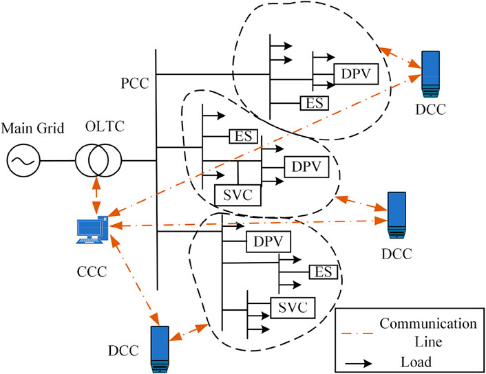
FIGURE 1. Connection diagram of the proposed control method.

The DCA collects the voltage information of each node in the regional DN and the power information of the incorporated voltage regulation equipment. The voltage unit value of each node can be calculated by Eq. 1:

$v_i=v_{i\_\mathrm{r}}\times v_{n,i}^{-1},(1)$

where $v_{i\_\mathrm{r}}$ is the voltage value of the bus node, $i$; $v_{n,i}$ is the nominal voltage of the $i-\text{th}$ bus node; the superscript “−1” means the bottom form; $v_i$ is the voltage per-unit value of the $i-\text{th}$ bus node. If the voltage of some bus nodes exceeds the voltage safety threshold, each DCA sends the value of the voltage standard to the CCA. The safety threshold is set at [.95, 1.05]p.u. After receiving the voltage information of all nodes, the CCA calculates the average unit value of the voltage standard, and if this value exceeds the set feeder threshold range, the OLTC splitter needs to be adjusted, and the feeder threshold range set at [.95, 1.05]p.u. Then, the DQN algorithm is used to obtain the optimal gear position of the OLTC splitter, which ensures that the unit value of the average voltage is kept within the safety threshold.

The aforementioned adjustment method can only ensure that the average standard unit value of voltage reaches the safety threshold. If the voltage of some bus nodes still exceeds the safety threshold range after adjusting the OLTC splitter, the power coordination control strategy based on the DPV, SVC, and ES output characteristics is adopted. The generalized node-based partitioning method is used to divide the control region of the DN (Zhang et al., 2014). In the region where the bus nodes are located, deep reinforcement learning is used to train the optimal power regulation sequence by coordinating the active and reactive power outputs of DPVs, the reactive power output of SVCs, and the ES output (Amir et al., 2022). The CCC determines the optimal control strategy and then issues commands to the CCC communicating with the area to adjust the power output of the inverter of each voltage regulation device. After receiving the instructions for executing the adjustments, the inverters guarantee that the voltage of each node is kept within the safety threshold, reducing the problem of bus node voltage overlimit. In the process of voltage regulation, the DPVs follow the principle that reactive power control voltage is first regulated before active power control voltage is cut, so as to give full play to the absorption capability of the PVs. According to the response times of DPVs, ES, and SVCs over the short timescale (Liu et al., 2022), the specific regulation priority is: OLTC > PV reactive power, ES, and SVC > PV active power. If it is necessary to reduce the active power of the DPVs, the active power reduction of a PV shall not exceed half of the DPV output active power. The overall control process is shown in Figure 2.

FIGURE 2

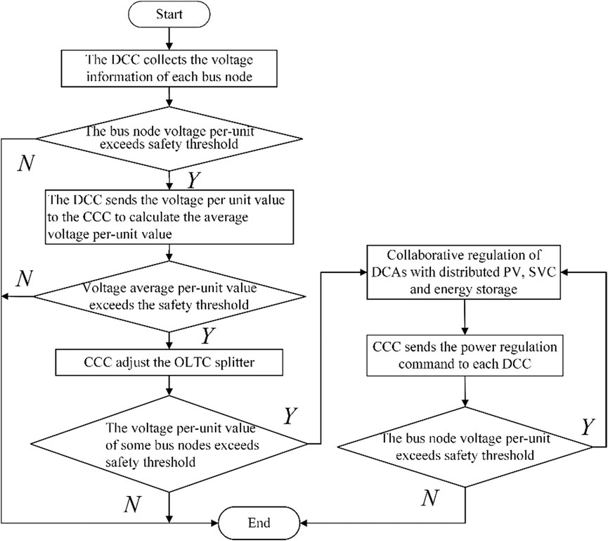
FIGURE 2. Overall framework of the cooperative voltage control strategy.

3 Modeling of voltage regulation devices on a DN

3.1 DPV inverter

As used in this paper, the DPV inverter adopts PQ control, and its controller is divided into inner and outer rings. The outer ring tracks the DC side of the active power output $p_{dc,ref}$ and the reference value of the reactive power output $q_{dc,ref}$, while the inner ring generates the SPWM modulation signal. The active and reactive power is calculated according to the output current and voltage after $dq$ conversion, and the voltage component of the shaft is obtained by PI control. Lastly, the output voltage of the inverter is obtained by voltage modulation (Atia et al., 2016; Vinnikov et al., 2018). The PQ control block diagram of a DPV inverter is shown in Figure 3.

FIGURE 3

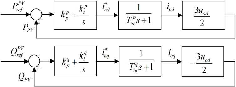
FIGURE 3. PQ control block diagram of the DPV inverter.

The active power output and the reactive power output of a model DPV inverter can be calculated as follows:

$\left\{\begin{array}{l}∆i_{od}=\frac{1}{T_{in}^{p}s+1}\left(k_p^p+\frac{k_i^p}{s}\right)∆P_{ref}^{PV}-∆P_{PV},\\ ∆P_{PV}=\frac{3u_{od}}{2}∆i_{od},\end{array}\right.(2)$

$\left\{\begin{array}{l}∆i_{oq}=\frac{1}{T_{in}^{q}s+1}\left(k_p^q+\frac{k_i^q}{s}\right)∆Q_{ref}^{PV}-∆Q_{PV},\\ ∆Q_{PV}=-\frac{3u_{od}}{2}∆i_{oq},\end{array}\right.(3)$

where $∆i_{od}$ and $∆i_{oq}$ are the differences between the components on axis $d$ and $q$ of the current and the previous time, respectively; $∆P_{PV}$ and $∆Q_{PV}$ are the differences between the current active power output and reactive power at the last time, respectively; and $∆P_{ref}^{PV}$ and $∆Q_{ref}^{PV}$ are the differences between the current active power output reference and the reactive power reference at the previous time, respectively. Thus, as long as the reference values of the active and reactive power outputs of the DPV inverter are adjusted, any changes in the grid-connected active and reactive components can be controlled.

3.2 OLTC

The OLTC regulates the voltage of the secondary side of the transformer by adjusting the location of the transformer connector, changing the ratio and the distribution of reactive power in the DN line (Wu et al., 2017). In this paper, the regulation of the on-load OLTC by the discrete variable ratio was used to control the voltage value of the secondary side of the transformer to keep it within the allowable range during operation. The adjusting process of the splitter is as follows:

$e={\mathit{V}}_1-{\mathit{V}}_{ref},(4)$

$t\left(\tau +1\right)=t\left(\tau \right)+∆T_{\tau },(5)$

$f\left(e,t\right)=\left\{\begin{array}{l}1\\ -1\\ 0\end{array}\right.\begin{array}{c}e>\frac{\epsilon }{2},t\ge T_d,\\ e<-\frac{\epsilon }{2},t\ge T_d,\\ \text{other},\end{array}(6)$

$n\left(t+1\right)=n\left(t\right)-d\cdot f\left(e\left(t\right),t\right),(7)$

where $e$ is the difference between the voltage value $V_1$ of the OLTC secondary side and the reference value $V_{ref}$; $t$ is a discrete moment during OLTC operation; $\tau$ is a counter; and $∆T_{\tau }$ is a constant determined by OLTC characteristics and voltage drop. After the OLTC has started to run from time $t$, if the time is ≥$∆T_{\tau }$, the counter will add one forward. $\epsilon$ is the voltage dead zone to avoid unnecessary actions when OLTC is operating within the permissible voltage range; $n$ is the location of the transformer splitter; $d$ is the number of gears changed by the OLTC splitter; and $T_d$ is the action delay time during OLTC operation.

3.3 SVC

The SVC used in this paper is a thyristor-controlled reactor model, and the control diagram is shown in Figure 4. The SVC is connected to the DN through an inverter, and the equivalent transfer function of the control loop of the inverter in reactive power control mode is given by the following formula (Chen et al., 2018):

$\left\{\begin{array}{l}∆B_{SVC}=\frac{1}{s{T}_{SVC}+1}∆u_{SVC},\\ ∆Q_{SVC}=∆B_{SVC}{U}_{SVC}^2,\end{array}\right.(8)$

where $∆B_{SVC}$ is the difference between the current and the equivalent susceptance at the previous time; $T_{SVC}$ is the time constant of the control loop; $∆u_{SVC}$ is the difference between the current and the control variable at the previous time; $U_{SVC}$ is the output voltage of the SVC inverter; and $∆Q_{SVC}$ is the difference between the current and the reactive power output of the previous time. It can be seen that SVC changes the SVC equivalent susceptance in the access system by controlling the trigger angle of the thyristor so as to adjust the reactive power.

FIGURE 4

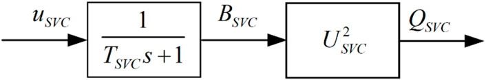
FIGURE 4. Equivalent transfer function of the control loop in the SVC.

3.4 ES battery

The ES system can be equivalent to a voltage source. Figure 5 shows the charging and discharging schematic diagram of the ES system (Yang et al., 2014; Gush et al., 2021), where $U_E$ and $U$ are, respectively, the voltage amplitude of the ES and the voltage amplitude of the connection point, and the voltage phase angles are $\theta$ and $\delta$, respectively. $I$ is the amplitude of the current injected into the grid by the ES, and the current phase angle is $\phi$; $R$ and $L$ are the resistance and induction in series in the line, respectively.

FIGURE 5

FIGURE 5. Charging and discharging schematic diagram of the ES battery.

ES uses SOC to represent the actual capacity of the battery at a certain time, and the ratio of the residual current $C_r$ to the stable capacity $C_{ba}$ is expressed as follows:

$SO{C}_t=\left(\frac{C_R}{C_{ba}}\right)\times 100\%.(9)$

SOC changes during the charging and discharging process as follows:

Battery discharging:

$SOC\left(t\right)=SOC\left(t-1\right)-\frac{P\left(t\right)\cdot ∆t}{C_{ba}\cdot {\eta }_{dis}}.(10)$

Battery charging:

$SOC\left(t\right)=SOC\left(t-1\right)+\frac{P\left(t\right)\cdot ∆t\cdot {\eta }_c}{C_{ba}},(11)$

where $P\left(t\right)$ is the ES output power at the $t-\text{th}$ time; ${\eta }_{dis}$ and ${\eta }_c$ are, respectively, the discharge efficiency and charging efficiency of ES; $SOC\left(t-1\right)$ is the ES SOC at the last moment; $∆t$ is the time interval. The power generated by ES and DPV needs to be converted from DC to AC through the inverter before injection into the power grid and is subject to PQ control. Therefore, as long as the reference values of the active and reactive power outputs of the ES inverter are adjusted, the changes in grid-connected active and reactive components can be controlled.

4 DQN-DDPG algorithm

4.1 Principles of the DQN algorithm

The DQN algorithm uses an experience playback mechanism, which stores the experience data $\left(s_t,a_t,r_t,s_{t+1}\right)$ obtained at each time point in the interaction process between the agent and the environment into the experience pool, and then randomly samples from the experience pool to reduce the correlation of the training data (Labash et al., 2020) so that it is easier to converge the agent training. The DQN algorithm establishes a separate target Q network and updates the weight parameter, $\theta$, of the Q network by constantly approximating the output $r+\gamma \underset{a^{\prime }}{\max }{Q}_{\pi }\left(s^{\prime },a^{\prime };{\theta }^{\prime }\right)$ of the target Q network and the output $Q_{\pi }\left(s,a;\theta \right)$ of the Q network. The loss function is defined and the weight parameter, $\theta$, is used to represent the mean squared error loss:

$L\left(\theta \right)=\underset{i\in M}{E}\left[(r_i+\gamma \underset{a^{\prime }}{\max }{Q}_{\pi }(s_i^{\prime },a^{\prime };{\theta }^{\prime })-Q_{\pi }(s_i,a_i;\theta ){)}^2\right],(12)$

where $E\left(\cdot \right)$ is the expected value; $r_i$ is the immediate reward of the $i-\text{th}$ group of data randomly sampled from the experience pool; $\gamma$ is the discount factor; and ${\theta }^{\prime }$ is the weight parameter of the target Q-network. The parameter, $\theta$, in the loss function is updated by the gradient descent method, and the algorithm expression is as follows:

${\theta }_{t+1}={\theta }_t+\alpha \left[r+\gamma \underset{a^{\prime }}{\max }{Q}_{\pi }\left(s^{\prime },a^{\prime };{\theta }^{\prime }\right)-Q\left(s,a;\theta \right)\right]\nabla Q_{\pi }\left(s,a;\theta \right),(13)$

where $\nabla$ is the gradient; ${\theta }_t$ and ${\theta }_{t+1}$ are the Q-network parameters at the $t-\text{th}$ time and the $\left(t+1\right)-\text{th}$ time, respectively; $\alpha$ is the step length; and $r$ is the value of the reward obtained. To ensure that the agent can simultaneously explore the unknown environment and the obtained environment information, an $\epsilon -greedy$ strategy is adopted to select the actions of the Q-network:

$\left\{\begin{array}{c}\begin{array}{cc}\text{select at random}\text{from}\mathrm{A}& \beta <\epsilon \end{array},\\ \begin{array}{cc}\underset{a\in \mathbf{A}}{\mathrm{a}\mathrm{r}\mathrm{g}\mathrm{m}\mathrm{a}\mathrm{x}{Q}_{\pi }\left(s,a;\theta \right)}& \beta \ge \epsilon \end{array},\end{array}\right.(14)$

where $\epsilon \in \left[\mathrm{0,1}\right]$ is a constant and $\beta \in \left[\mathrm{0,1}\right]$ is a random number.

4.2 Principles of the DDPG algorithm

The DDPG algorithm was based on and developed from the DQN algorithm. It mainly uses an actor network to make up for the shortcoming that DQN cannot deal with continuous control problems. The DDPG is an algorithm based on the ‘actor-critic’ architecture to obtain the optimal control sequence. In the actor-critic architecture, the actor network takes the state vector as the input, and the action vector as the output. The critic network takes the state and the action vector as the input, and the estimated Q value is the output (Sutton and Barto, 2018; Qin et al., 2022). The output of the network obtains the maximum value of Q. At the same time, the actor target network and the critic target network are established to output the target Q value, and the optimization training is completed by minimizing the difference between the target Q values and the target Q value. The relationship between actor and critic networks is shown in Figure 6.

FIGURE 6

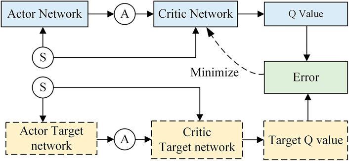
FIGURE 6. Diagram of the relationship between the actor and critic networks.

The actor network obtains the current state from the environment and outputs a definite action $\mu \left(s_t\left|{\theta }^{\mu }\right.\right)$ through the deterministic policy gradient method, where ${\theta }^{\mu }$ is the weight coefficient of the actor network. However, one disadvantage is that the environment cannot be fully explored because of the small amount of sampled data, so random noise $N_t$ is introduced in the output action. The $OU$ random process in this algorithm is selected to stimulate the ability of the agent to explore the optimal policy in the environment. The DDPG algorithm also uses the experience playback mechanism to store the experience data $\left(s_t,a_t,r_t,s_{t+1}\right)$ into the experience pool, so that the $W$ groups of experience data sampled randomly are trained.

The algorithm updates the parameters of the critic network by minimizing the loss function $L=\frac{1}{W}{\sum }_i\left({y_i-Q\left(s_i,a_i\left|{\theta }^Q\right.\right)}^2\right)$, where ${\theta }^Q$ is the weight parameter of the critic network, $Q\left(s_i,a_i\left|{\theta }^Q\right.\right)$ is the output Q value of the critic network, $y_i=r_i+\gamma Q^{\prime }\left(s_{i+1},{\mu }^{\prime }\left(s_i+1\left|{\theta }^{{\mu }^{\prime }}\right.\right);{\theta }^{Q^{\prime }}\right)$ is the long-term cumulative reward, ${\theta }^{Q^{\prime }}$ is the weight parameter of the critic target network, and ${\theta }^{{\mu }^{\prime }}$ is the weight coefficient of the actor target network. $Q^{\prime }\left(s_{i+1},{\mu }^{\prime }\left(s_i+1\right)\left|{\theta }^{Q^{\prime }}\right.\right)$ is the target Q value of the output of the critic target network, and $r_i$ is the immediate reward obtained by the critic target network. The algorithm updates the parameters of the actor network through the policy gradient method:

${\left.{\left.{\left.{\nabla }_{{\theta }^{\mu }}J\right|}_{s_i}\approx \frac{1}{W}{\displaystyle \sum }_i{\nabla }_{a}Q\left(s,a\left|{\theta }^Q\right.\right)\right|}_{s=s_i,a=\mu \left(s_i\right)}{\nabla }_{{\theta }^{\mu }}\mu \left(s\left|{\theta }^{\mu }\right.\right)\right|}_{s_i}.(15)$

Finally, by a $softupdate$, which updates the parameters of the critic target network and the actor target network,

$\left\{\begin{array}{c}{\theta }_t^{Q^{\prime }}=\eta {\theta }_t^Q+\left(1-\eta \right){\theta }_{t-1}^Q,\\ {\theta }_t^{{\mu }^{\prime }}=\eta {\theta }_t^{\mu }+\left(1-\eta \right){\theta }_{t-1}^{\mu },\end{array}\right.(16)$

where $\eta$ is the divergence factor, $0<\eta <1$; ${\theta }_t^Q$ and ${\theta }_t^{Q^{\prime }}$ are the critic network parameters and the critic target network parameters at the $t-\text{th}$ time, respectively; and ${\theta }_t^{\mu }$ and ${\theta }_t^{{\mu }^{\prime }}$ are the actor network parameters and the actor target network parameters at the $t-\text{th}$ time, respectively.

5 Voltage cooperative control method for a DN based on the DQN-DDPG algorithm

Combined with the multi-time scale voltage coordination control framework described in the second part, the voltage cooperative control architecture based on the DQN-DDPG algorithm can be divided into a top algorithm layer and a bottom control layer, as shown in Figure 7.

FIGURE 7

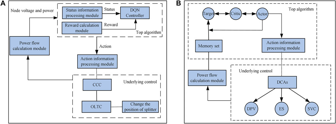
FIGURE 7. Voltage control architecture based on DQN-DDPG; (A) DQN algorithm; (B) DDPG algorithm.

5.1 Mathematical model of voltage control

In adjusting the OLTC splitter, the control objective is to minimize the average voltage exceedances of the bus nodes in the whole DN:

$\min F\left(x\right)=\left\{\begin{array}{cc}\overline{U}-1.05{\overline{U}}_N,& \overline{U}\ge 1.05{\overline{U}}_N,\\ 0.95{\overline{U}}_N-\overline{U},& \overline{U}\le 0.95{\overline{U}}_N,\end{array}\right.(17)$

where $\overline{U}$ is the average voltage of bus nodes in the whole DN; ${\overline{U}}_N$ is the average voltage rating of the DN; $N$ is the number of bus nodes in the whole DN; and $\pm 5\%$ is the safety threshold range of average bus node voltage per unit value set. When adjusting the voltage of some nodes in the control area, the control objective is to minimize the over-limit values of the bus node voltage in the control area:

$\min F\left(x\right)=\left\{\begin{array}{c}{\displaystyle \sum }_{i=1}^M\left(U_i-1.05U_N\right),U_i\ge 1.05U_N,\\ {\displaystyle \sum }_{i=1}^M\left(0.95U_N-U_i\right),U_i\le 0.95U_N,\end{array}\right.(18)$

where $U_i$ is the node voltage of the $i-\text{th}$ node; $U_N$ is the rated voltage of the DN; $M$ is the number of DN bus nodes in the control region; and $\pm 5\%$ is the maximum safe voltage range.

The constraints are as follows:

1) Power flow constraints

$\left\{\begin{array}{l}{\displaystyle \sum }_{i=1}^M{P}_{i,l}\left(t\right)+P_{loss}\left(t\right)=P_M\left(t\right)+P_{i,PV}\left(t\right)+P_{i,ES}\left(t\right),\\ {\displaystyle \sum }_{i=1}^M{Q}_{i,l}\left(t\right)+Q_{loss}\left(t\right)=Q_M\left(t\right)+Q_{i,PV}\left(t\right)+Q_{i,SVC}\left(t\right),\end{array}\right.(19)$

where $P_{i,l}\left(t\right)$ and $Q_{i,l}\left(t\right)$ are the active power and reactive power consumed by the load at the $t-\text{th}$ time of the $i-\text{th}$ node, respectively; $P_{loss}\left(t\right)$ and $Q_{loss}\left(t\right)$ are the active and reactive power losses of the DN line at the $t-\text{th}$ time, respectively; $P_M\left(t\right)$ and $Q_M\left(t\right)$ are the active power and reactive power emitted by the main network at the $t-\text{th}$ time, respectively; $P_{i,PV}\left(t\right)$ and $Q_{i,PV}\left(t\right)$ are the active power output and the reactive power output of the DPV at the $t-\text{th}$ time, respectively; $P_{i,ES}\left(t\right)$ is the ES active power output at the $t-\text{th}$ time of the $i-\text{th}$ node; and $Q_{i,SVC}\left(t\right)$ is the reactive power output of SVC at the $t-\text{th}$ time of the $i-\text{th}$ node.

2) ES output constraints

$\left\{\begin{array}{c}{P}_{i,\min }^{ES}\left(t\right)\le P_i^{ES}\left(t\right)\le P_{i,\max }^{ES}\left(t\right),\\ ∆P_{i,\min }^{ES}\left(t\right)\le ∆P_i^{ES}\left(t\right)\le ∆P_{i,\max }^{ES}\left(t\right),\end{array}\right.(20)$

where $P_i^{ES}\left(t\right)$ and $\Delta P_i^{ES}\left(t\right)$ are the ES active power outputs and active power output increases at the $t-\text{th}$ time of the $i-\text{th}$ node, respectively; $P_{i,\min }^{ES}\left(t\right)$ and $P_{i,\max }^{ES}\left(t\right)$ are the upper and lower limits of the ES active power outputs at the $t-\text{th}$ time of the $i-\text{th}$ node, respectively; $∆P_{i,\min }^{ES}\left(t\right)$ and $∆P_{i,\max }^{ES}\left(t\right)$ are the active power output increases at the upper and lower limit at the $t-\text{th}$ time of the $i-\text{th}$ node, respectively.

3) SOC constraints of ES

$\left|SO{C}_i-SO{C}_{ref}\right|\le {\epsilon }_{\text{ES}},(21)$

where $SO{C}_{ref}$ and $SO{C}_i$ are the reference values for the ES SOC and the SOC at the $i-\text{th}$ node, respectively, and ${\epsilon }_{\text{ES}}$ is the convergence error threshold of the ES SOC consistency protocol.

4) SVC output constraints

$\left\{\begin{array}{c}{Q}_{i,\min }^{SVC}\left(t\right)\le Q_i^{SVC}\left(t\right)\le Q_{i,\max }^{SVC}\left(t\right),\\ ∆Q_{i,\min }^{SVC}\left(t\right)\le ∆Q_i^{SVC}\left(t\right)\le ∆Q_{i,\max }^{SVC}\left(t\right),\end{array}\right.(22)$

where $Q_i^{SVC}\left(t\right)$ and $∆Q_i^{SVC}\left(t\right)$ are the SVC active power outputs and active power output increases at the $i-\text{th}$ node, respectively; $Q_{i,\min }^{SVC}\left(t\right)$ and $Q_{i,\max }^{SVC}\left(t\right)$ are the lower and upper limits of SVC reactive output at the $i-\text{th}$ node, respectively; $∆Q_{i,\min }^{SVC}\left(t\right)$ and $∆Q_{i,\max }^{SVC}\left(t\right)$ are the SVC active power output increases at the lower and upper limits at the $t-\text{th}$ time of the $i-\text{th}$ node, respectively.

5) Regulation constraints of the OLTC splitter

$D_{\min }\le D\le D_{\max },(23)$

where $D$ is the splitter position of the OLTC, and $D_{\min }$ and $D_{\max }$ are the lower and upper limits of the OLTC splitter tap, respectively.

5.2 Design of the DQN-DDPG algorithm

5.2.1 Long timescale DQN algorithm

5.2.1.1 State space

The objective of the voltage control strategy in this paper was to modulate the voltage of the bus nodes. The power input of each node needs to be monitored in real time, and the OLTC splitter needs to be adjusted accordingly. Therefore, the state space of the DQN algorithm was defined as the voltage of each bus node in the DN:

$S_{DQN}=\left\{v_1,v_2,\cdots ,v_i,\cdots v_N\right\},(24)$

where $v_i$ is the per-unit value of the $i-\text{th}$ node voltage, $1\le i\le N$.

5.2.1.2 Action space

The voltage amplitude is changed by changing the tap position of the OLTC splitter, so the action space $A_{DQN}$ of the DQN algorithm is defined from this tap position, and it is assumed that the OLTC splitter has $n$ tap positions and the adjustment range is $\pm n\times 1\%\mathrm{p}.\mathrm{u}.$, and each tap position is adjusted as $i\times 1\%\mathrm{p}.\mathrm{u}.$, $-n\le i\le n$. The expression is as follows:

$A_{DQN}=\left\{-n\times 1\%\mathrm{p}.\mathrm{u}.,-\left(n-1\right)\times 1\%\mathrm{p}.\mathrm{u}.,\cdots ,0\%\mathrm{p}.\mathrm{u}.,\cdots ,\left(n-1\right)\times 1\%\mathrm{p}.\mathrm{u}.,n\times 1\%\mathrm{p}.\mathrm{u}.\right\}.(25)$

5.2.1.3 Reward function

The centralized cooperative controller calculates the average per-unit value of the voltage after receiving voltage information from the bus nodes in the whole DN. If the average per-unit value of voltage exceeds the safety threshold, that is, [.95,1.05]p.u., it is adjusted by the OLTC splitter. Therefore, the immediate reward function is as follows:

$r_{DQN,i}=-{\alpha }_{\mathrm{w}}∆{{\overline{v}}_i}^2,(26)$

where ${\alpha }_{\mathrm{w}}$ is the weight coefficient and $\Delta \overline{v}$ is the value where the average per-unit value of the voltage of the bus nodes in the DN exceeds the safety threshold, specifically:

$∆{\overline{v}}_i=\left\{\begin{array}{c}{\overline{v}}_i-0.95,{\overline{v}}_i>0.95,\\ 1.05-{\overline{v}}_i,{\overline{v}}_i<1.05,\end{array}\right.(27)$

where ${\overline{v}}_i$ is the average per-unit value of the voltage at the bus nodes in the whole DN.

5.2.2 Short timescale DDPG algorithm

5.2.2.1 State space

The DDPG algorithm is mainly used to prevent voltage control problems in the DN area where the voltage overlimit nodes are located. Therefore, the DDPG state space is different from that of DQN algorithm, and the power output of each node in this area needs to be collected in real time to follow up on the regulation of power output by the voltage regulation equipment. Therefore, the state space of the DDPG algorithm is defined as follows:

$S_{DDPG,i}=\left\{v_1,\cdots ,v_i,\cdots ,v_M,p_1,\cdots ,p_i,\cdots ,p_M,q_1,\cdots ,q_i,\cdots ,q_M\right\},(28)$

where $v_i$ is the per-unit value of the $i-\text{th}$ node voltage; $p_i$ is the active power of the $i-\text{th}$ node; $q_i$ is the reactive power of the $i-\text{th}$ node, $1\le i\le M$; and $M$ is the number of bus nodes in the DN region.

5.2.2.2 Action space

If the voltage at some nodes still exceeds the safety threshold after adjusting the OLTC splitter according to the DQN algorithm, then the active and reactive power outputs of the DPVs, the ES output, and the reactive power output of the SVCs in the control region where the node is located can be adjusted to control the voltage. The action space of the DDPG algorithm is defined as follows:

$A_{DDPG,i}=\left\{A_i^{PV},A_i^{ES},A_i^{SVC}\right\}.(29)$

When only DPV reactive power regulation is used, $A_i^{PV}=∆Q_i^{PV}$. If regulation of the reactive power cannot achieve the desired voltage control, then DPV active power reduction is added and $A_i^{PV}=\left\{∆P_i^{PV},∆Q_i^{PV}\right\}$; similarly, $A_i^{ES}=∆P_i^{ES}$, $A_i^{SVC}=∆Q_i^{SVC}$; where $∆P_i^{PV}$ and $∆Q_i^{PV}$ are the variations in the active and reactive power outputs of DPVs at the $i-\text{th}$ node; $∆P_i^{ES}$ is the variation in the active power output of ES at the $i-\text{th}$ node; and $∆Q_i^{SVC}$ is the variation in SVC reactive power output at the $i-\text{th}$ node. The power output of each voltage regulation device must comply with the corresponding following constraints.

5.2.2.3 Reward function

The DDPG algorithm controls the voltage of each node by adjusting the outputs of the DPVs, ES, and SVCs connected to each node. The control objective is to stabilize the voltage and keep it from exceeding the safety threshold; thus, the immediate reward function is set as the sum of the quadratic form of the higher limit voltage of each node, the active power and reactive power regulation of the DPV output, the active power regulation of the ES output, and the reactive power regulation of the SVC output:

$\begin{array}{l}{r}_{DDPG,i}=-∆v_{i_v}\cdot B\cdot ∆{v_{i_v}}^T-{\eta }_s∆P_{i_{pv}}^{PV}\cdot C\cdot ∆P_{i_{pv}}^{P{V}^T}-∆Q_{i_{pv}}^{PV}\cdot C\cdot ∆Q_{i_{pv}}^{P{V}^T}\\ -∆P_{i_{es}}^{ES}\cdot D\cdot ∆P_{i_{es}}^{E{S}^T}-∆Q_{i_{svc}}^{SVC}\cdot E\cdot ∆Q_{i_{svc}}^{SV{C}^T}\\ \forall i_v\in M,\forall i_{pv}\in {\mathbb{N}}_{PV},\forall i_{es}\in {\mathbb{N}}_{ES},\forall i_{svc}\in {\mathbb{N}}_{SVC},\end{array}(30)$

where $∆v_i$ is the voltage limit of the $i-\text{th}$ bus node; $M$ is the number of bus nodes in the control region; and ${\mathbb{N}}_{PV}$, ${\mathbb{N}}_{ES}$, and ${\mathbb{N}}_{SVC}$ are the number of DPVs, ES, and SVCs in the control region, respectively. The matrices $B$, $C$, $D$, and $E$ are all weight matrices; ${\eta }_s$ is the selection coefficient, and when DPV active power reduction is not used, $\eta =0$; when PV active power reduction is added, $\eta =1$.

5.3 Overall flow of the algorithm

1) The iterative process of OLTC tap adjustment based on DQN is as follows:

S1: Calculate the average standard per-unit value of voltage according to DN environment. If the average standard value of voltage exceeds the safety threshold, the DQN agent will be trained at the initial position of the OLTC splitter.

S2: The standard unit value of voltage at each bus node in the DN obtained by the CCC is taken as the set, $s_t=\left\{v_1,v_2,\cdots ,v_N\right\}$, of the initial states of the DQN agent.

S3: Select the corresponding action $a_t$ of the OLTC splitter tap from the action set $A_{DQN,i}$ according to the $\epsilon -greedy$ strategy, and execute the action $a_t$ to obtain the immediate reward according to the reward function, $r_{DQN,i}$. The updated per-unit value of voltage of each bus node obtained by the MATPOWER power flow calculation is the next state set $s_{t+1}$, and the experience data set, $\left(s_t,a_t,r_t,s_{t+1}\right)$, is stored in the experience pool (Zimmerman et al., 2011).

S4: Sampling the empirical data set randomly from the experience pool according to the sampled data set, $\left(s_j,a_j,r_j,s_{j+1}\right)$.

S5: After updating the state set, the per-unit value of the bus node changes, and it must be recalculated to determine if the average per-unit value of the voltage meets the conditions of the safety threshold [.95,1.05]p.u. If the conditions are met, the iteration will be terminated. The target Q value $y_j$ is substituted into the current immediate reward, $r_j$. If the condition is not met, the objective Q value $y_j$ is substituted into the long-term cumulative reward value, $r_j+\gamma {\max }_{a^{\prime }}{Q}_{\pi }\left(s_{j+1},a^{\prime };\theta \prime \right)$.

S6: Use the gradient descent method to update the parameter $\theta$ in the loss function.

S7: Update the parameters, ${\theta }^{\prime }=\theta$, of the target Q network at every other iteration.

S8: Continue to perform S3 until the set of states meets the termination iteration condition.

2) If the standard voltage value of some bus nodes is still beyond the safety threshold [.95,1.05] after adjusting the OLTC splitter by DQN algorithm, the output power of DPVs, ES, and SVCs should be optimized and adjusted by the DDPG algorithm. The specific control process is as follows:

S1: The per-unit value of the voltage and the power information from all bus nodes in the control region where the overlimit bus node is located are used as the initial state set, $s_t=\left\{v_1,v_2,\cdots ,v_M,p_1,p_2,\cdots ,p_M,q_1,q_2,\cdots ,q_M\right\}$, of the DDPG algorithm.

S2: Select the actions, $a_t=\mu \left(s_t\left|{\theta }^{\mu }\right.\right)+N_t$, corresponding to the DPV, ES, and SVC output power according to the current strategy and random noise, $A_{DDPG,i}$, and execute the actions $a_t$ to obtain immediate rewards $r_t$ according to the reward function $r_{DDPG,i}$. After MATPOWER power flow calculations, the updated voltage per-unit value, the active power, and the reactive power at each bus node are taken as the next state set, $s_{t+1}$, and the empirical data set, $\left(s_t,a_t,r_t,s_{t+1}\right)$, is stored in the experience pool.

S3: $W$ groups of empirical data sets are randomly sampled from the experience pool, and the target Q value, $y_i=r_i+\gamma Q\prime \left(s_{k+1},\mu \prime \left(s_{k+1}\left|{\theta }^{{\mu }^{\prime }}\right.\right)\left|{\theta }^{Q^{\prime }}\right.\right)$, of the output of the critic objective function is calculated according to the sampled data, $\left(s_k,a_k,r_k,s_{k+1}\right)$.

S4: The critic network parameters are updated by minimizing the loss function, $L=\frac{1}{W}{\sum }_i\left({y_i-Q\left(s_i,a_i\left|{\theta }^Q\right.\right)}^2\right)$, and the actor network parameters are updated by the policy gradient method.

S5: Update the critic target network parameters ${\theta }^{Q^{\prime }}$ and the actor target network parameters ${\theta }^{{\mu }^{\prime }}$ according to the $softupdate$ method.

S6: If the standard value of the bus node voltage in the control region lies within the safety threshold [.95, 1.05]p.u., the iteration ends. If the conditions are not met, perform Step 3.

6 The simulation verification

6.1 Example introduction

To verify the effectiveness of the cooperative voltage optimization control method considering the load and storage of the source network proposed in this paper, the improved IEEE 33-node DN system was adopted to perform a simulation analysis on a MATLAB r2019a platform. The improved topology diagram of the DN is shown in Figure 8. The total load was 3715.0 kW + j2300.0kVar, and the rated voltage was 10 kV in the DN. The node loads and generator parameters in the DN system are shown in Table 1, and the DN branch parameters are shown in Table 2. The OLTC of the DN is located at node 1, its rated capacity is 100MVA, and the adjustment range is $\pm 5\times 1\%\mathrm{p}.\mathrm{u}.$ The DPVs are located at nodes 18, 19, and 33, and the rated PV capacity is 2.2 MW. The ES are located at nodes 12, 15, 22, and 28 with a rated capacity of $800\text{kW}\cdot \mathrm{h}$, a maximum charge–discharge power of 400 kW, and a convergence error threshold of .05. The SVCs are located at nodes 17 and 25, and the maximum capacity is 2MVar. The safety threshold of the bus node voltage per-unit value is set as [.95,1.05]p.u. According to the DN control region division method, the DN is partitioned, as shown in Figure 6.

FIGURE 8

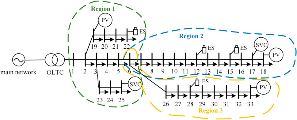
FIGURE 8. DN topology of the IEEE-33 node.

TABLE 1

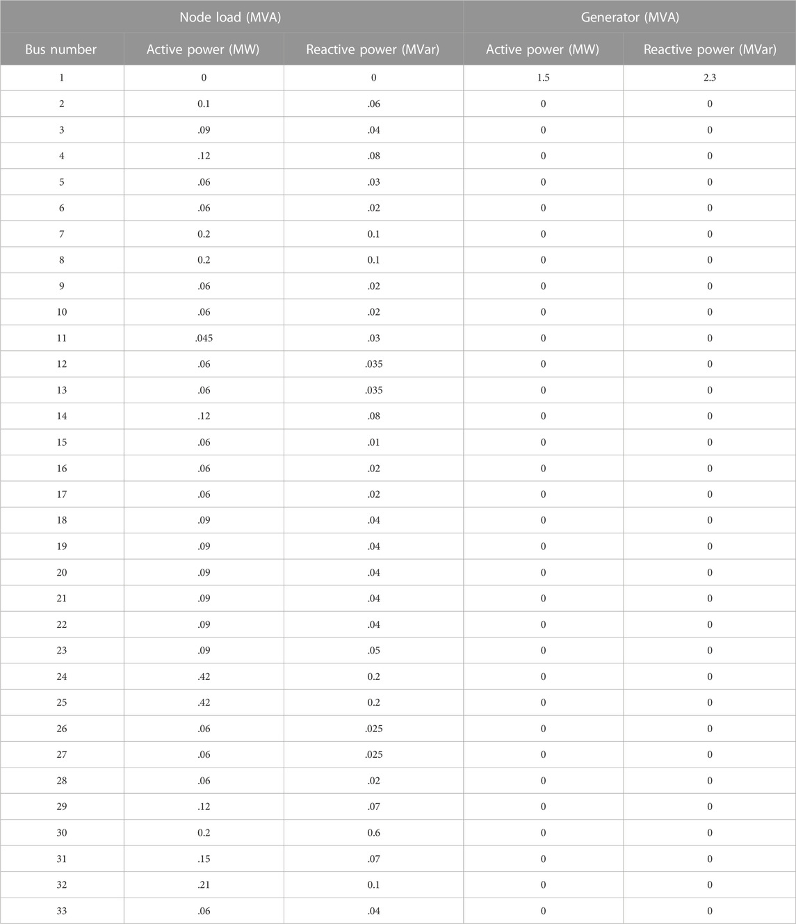
TABLE 1. Load and generator parameters of the standard IEEE 33-node DN system.

TABLE 2

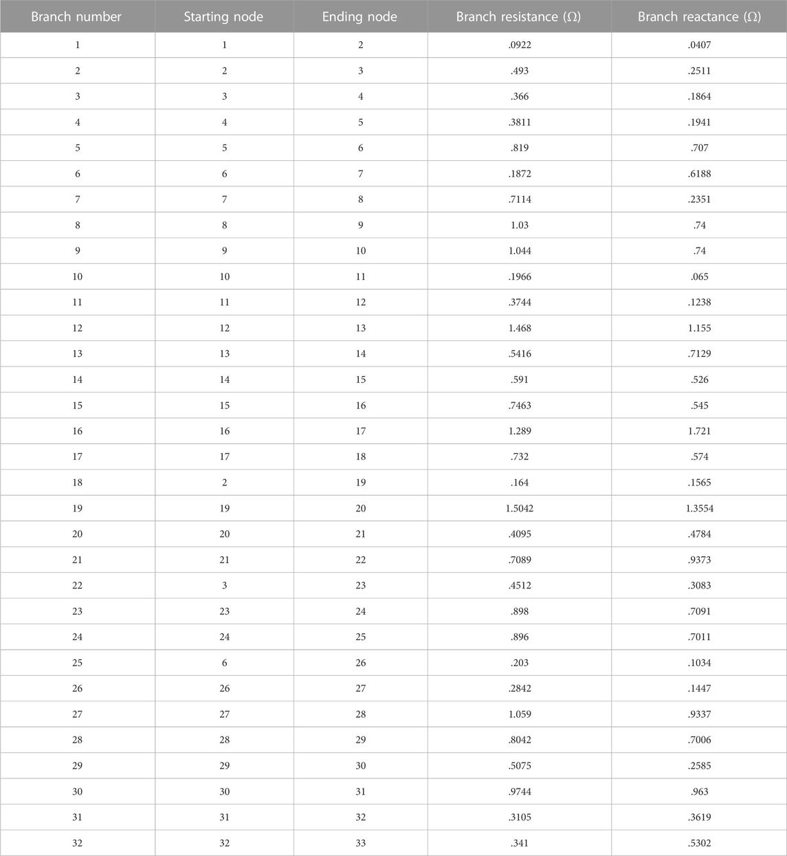
TABLE 2. Branch parameters of the standard IEEE 33-node DN system.

6.2 Analysis of simulation results

The power disturbance was introduced into the DN at a certain time, and the voltage amplitude of each node is shown in Figure 7.

Overvoltage events occurred at nodes 9–18, 32, and 33 (Figure 9). The DQN algorithm was first designed according to the regulation range of the OLTC:

• State Space. There are 33 bus nodes in the whole-domain DN, and the state space of the DQN algorithm can be obtained by using Eq. 24, $S_{DQN}=\left\{v_1,v_2,\cdots ,v_i,\cdots v_{33}\right\}$.

• Action Space. The regulation range of the OLTC is $\pm 4\times 1\%\mathrm{p}.\mathrm{u}.$ There are 9 splitter taps, the reference per-unit value of bus node is 1, and the action space of the DQN algorithm can be obtained according to Eq. 25:

$\begin{array}{l}{A}_{DQN}=\left\{-4\%\mathrm{p}.\mathrm{u}.,-3\%\mathrm{p}.\mathrm{u}.,-2\%\mathrm{p}.\mathrm{u}.,-1\times 1\%\mathrm{p}.\mathrm{u}.,0\%\mathrm{p}.\mathrm{u}.,1\%\mathrm{p}.\mathrm{u}.,2\%\mathrm{p}.\mathrm{u}.,3\%\mathrm{p}.\mathrm{u}.,4\%\mathrm{p}.\mathrm{u}.\right\}\\ =\left\{0.96\mathrm{p}.\mathrm{u}.,0.97\mathrm{p}.\mathrm{u}.,0.98\mathrm{p}.\mathrm{u}.,0.99\mathrm{p}.\mathrm{u}.,1\mathrm{p}.\mathrm{u}.,1.01\mathrm{p}.\mathrm{u}.,1.02\mathrm{p}.\mathrm{u}.,1.03\mathrm{p}.\mathrm{u}.,1.04\mathrm{p}.\mathrm{u}.\right\}.\end{array}(31)$

• Reward Function. The purpose of the OLTC splitter is to keep the average per-unit value of the voltage in the DN within the safety threshold range. According to Eq. 26, the reward function of the DQN algorithm can be obtained as follows:

$\begin{array}{l}{r}_{DQN}=-\Delta {\overline{v}}^2\times {10}^5\\ \Delta \overline{v}=\left\{\begin{array}{l}\frac{v_1+\cdots +v_i+\cdots +v{}_{33}}{33}-0.95\\ 1.05-\frac{v_1+\cdots +v_i+\cdots +v{}_{33}}{33}\end{array}\right.\begin{array}{c}\frac{v_1+\cdots +v_i+\cdots +v{}_{33}}{33}\ge 0.95,\\ \frac{v_1+\cdots +v_i+\cdots +v{}_{33}}{33}<1.05.\end{array}\end{array}(32)$

FIGURE 9

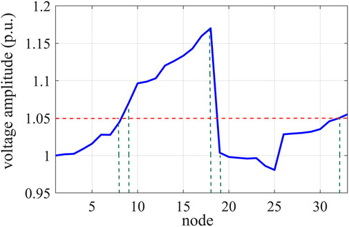
FIGURE 9. Voltage amplitude of each bus node without control.

The learning rate of the neural network was chosen as .001, the discount coefficient was .99, the capacity of the experience pool was 4,000, and the capacity of the mini-batch was 64. DQN agents were trained with a total of 500 episodes, and each episode was completed after 300 samples were trained. The results of training the agents according to the iterative process of algorithm 4.1 are shown in Figure 10. The episode reward is the cumulative reward value in an episode obtained by the agent during training, and the average reward is the average of the reward values in every four episodes. As can be seen from Figure 8, at the beginning of the training, the reward value was very low due to the limited learning experience. As the training continued, the agents kept exploring and learning, and the reward value kept increasing. After 250 episodes, the reward value of the DQN agent fluctuated within a small range, which indicated that the algorithm gradually converged and the agents’ training had developed an optimal strategy for controlling the voltage by adjusting the OLTC splitter.

FIGURE 10

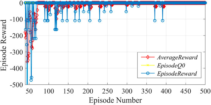
FIGURE 10. DQN agent training process.

During the test, the OLTC training data were used as the control. Figure 11 shows the effects of adjusting the OLTC splitter, at which point the OLTC splitter was set at $-3\times 1\%\mathrm{p}.\mathrm{u}.$ It can be seen that the voltage amplitude of each bus decreased, but there were still some bus nodes whose voltage standard value exceeded the safety threshold. Therefore, it was necessary to readjust the voltage through DPV, ES, and SVC regulation in the area where it exceeded the limit.

FIGURE 11

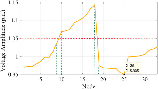
FIGURE 11. Voltage amplitude of each bus node after adjusting OLTC.

The DDPG algorithm was then applied according to the DPV, ES, and SVC in the region where the voltage overlimit node is located.

• State Space. Control region 2 contains 13 bus nodes. As can be seen from Figure 11, after adjusting the OLTC splitter, the standard voltage values at nodes 9, 32, and 33 were controlled within the safety threshold, but the voltages at nodes 10–18 were still beyond the upper limit of the safety threshold. According to Eq. 28, the state space of the DDPG algorithm can be obtained as follows:

$S_{DDPG}=\left\{v_1,\cdots ,v_i,\cdots ,v_{13},p_1,\cdots ,p_i,\cdots ,p_{13},q_1,\cdots ,q_i,\cdots ,q_{13}\right\}1\le i\le 13.(33)$

• Action Space. Node 18 incorporates DPV, nodes 12 and 15 are ES, and node 17 is SVC. The DDPG action space can be obtained according to Eq. 29:

$\left\{\begin{array}{l}{A}_{DDPG}=\left\{A_i^{PV},A^{ES},A^{SVC}\right\},\\ A_i^{PV}=\left\{∆P^{PV},∆Q^{PV}\right\},\\ A^{ES}=\left\{∆P_i^{ES}\right\}1\le i\le 2,\\ A^{ES}=\left\{∆Q^{SVC}\right\}.\end{array}\right.(34)$

According to variations in the active power output of DPVs, the adjustable range of the DPV reactive power can be obtained as follows:

$\Delta Q=\left[-\sqrt{S^2-P_{PV}^2},\sqrt{S^2-P_{PV}^2}\right].(35)$

According to the SOC consistency protocol for ES, the SOC reference value is .5, the convergence error threshold is .02, and the charge–discharge efficiency is 80%.

• Reward Function. The DDPG algorithm controls node voltage by regulating the DPVs, ES, and SVCs connected in Region 2. The reward function can be expressed by Eq. 30:

$\begin{array}{l}{r}_{DDPG}=-∆v_{i_v}\cdot B\cdot ∆{v_{i_v}}^T-∆P^{PV}\cdot C\cdot ∆P^{P{V}^T}-∆Q^{PV}\cdot C\cdot ∆Q^{P{V}^T}\\ -∆P_{i_{es}}^{ES}\cdot D\cdot ∆P_{i_{es}}^{E{S}^T}-∆Q^{SVC}\cdot E\cdot ∆Q^{SV{C}^T}1\le i_v\le \mathrm{13,1}\le i_{es}\le 2,\end{array}(36)$

where $B=100*{\mathbf{I}}_{13\times 13}$, $D=10\times {\mathbf{I}}_{2\times 2}$, and $C=E=10$ constitute the weight matrix and $\mathbf{I}$ is the identity matrix.

The parameters of the DDPG algorithm for the neural network were set as follows. The learning rate of the actor network was .001, the learning rate of the critic network was .0001, the discount coefficient was .99, the update coefficient was .01, and the capacity of the experience pool was 4,000. The capacity of the mini-batch was selected as 64, and the noise variable was .3. The DDPG agent was trained with 1,000 episodes according to the iterative process of algorithm 4.2 and each episode involved training 300 samples (Figure 12). It can be seen at the beginning of the training that the reward value was very low due to the limited learning experience. As the training continued, the agent kept exploring and learning, and the reward value kept increasing. After 800 episodes, the reward value of the DDPG agent fluctuated very little within a small range, which indicated that the algorithm gradually converged; the agent’s exercise training had developed an optimal strategy for voltage control of DPV and ES in the regulation region.

FIGURE 12

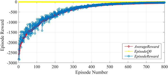
FIGURE 12. DDPG agent training process.

To make full use of the active DPV power consumption capacity, the DPV reactive power and ES were regulated. During the test, the power output training data on the voltage regulation equipment were used as control. Figure 13 shows the effect of controlling nodes 9–18 without reducing the active DPV power. It can be seen that the bus contact voltage in this control region at this time was not regulated within the safety threshold. Thus, DPV reactive power and ES cannot achieve the desired voltage control, so the active power must be further reduced. Figure 14 shows the voltage control effect of nodes 9–18 with active power reduction, and Figure 15 shows the level of power adjustment of each voltage regulation device in this control region.

FIGURE 13

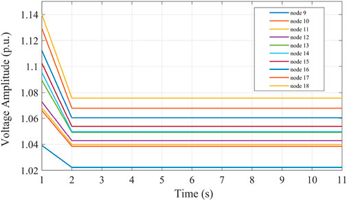
FIGURE 13. Voltage control effect in the case of no active power reduction.

FIGURE 14

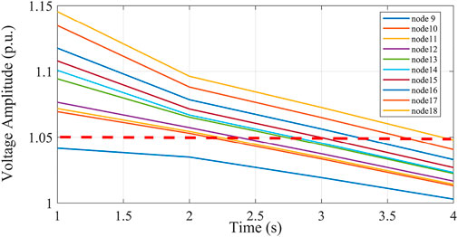
FIGURE 14. Voltage control effect when active power reduction is added.

FIGURE 15

FIGURE 15. Power adjustments of each voltage regulation device.

The DDPG algorithm was used for voltage control for 0.04 s. According to Figures 14, 15, the ES was discharged, and the output active power was about 250 KW. The SVC reactive power output was about 537.3 kVar, the DPV reactive power output was 372.8 kVar, and the active power reduction was less than 200 KW. The consumption capacity of the DPVs in the DN can be improved by reducing the active power reduction of the DPVs as much as possible. By adjusting the output power of the DPVs and the ES in the control region, the voltage of the bus node can be quickly and effectively maintained within the safety threshold.

To demonstrate the advantages of the rapid calculation speed of the DQN-DDPG algorithm, this paper compared it with the PSO algorithm. Figure 16 shows the effect of testing the voltage control model using the PSO algorithm with a consumption time of 19.52 s, and it is obvious that the DDPG algorithm was able to control voltage more quickly. This is because the PSO must obtain the optimal control strategy through continuous iteration, and the solution process was an iterative process of the objective function, while DDPG achieved the optimal strategy through the exploration and learning of the environment by the agents; the optimal strategy was the trained optimization sequence.

FIGURE 16

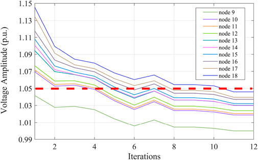
FIGURE 16. Voltage control effects of the PSO algorithm.

7 Conclusion

In order to give full play to the voltage regulating potential of the high permeability DGs in the DN, a deep reinforcement learning algorithm was used to test the voltage control model of the corresponding DN. The voltage control model was converted to a Markov decision process, and the whole series of steps of the algorithm to improve its design depth according to the objective function and constraint conditions were put forward. By combining the DQN and the DDPG algorithms with deep reinforcement learning, the discrete and continuous variables could be processed simultaneously, and the algorithms could control the DN in real time according to the current state of the power grid. The algorithms were independent of changes in the DN environment, and the optimal strategy was obtained through the exploration and learning of agents in the environment. This method effectively solved the problems of large model dimensions and high data volumes, to complete complex tasks, and achieve cooperative control of different voltage regulation devices.

However, this paper still has some imperfections. When the controller issues voltage regulation instructions to the inverter, there is an unavoidable communication delay, which can affect the real-time performance and effectiveness of the voltage regulation equipment. Also, this paper only considered a DN with OLTC, DPV, ES and SVC access, and did not conduct in-depth research on newer DNs with large-scale access to wind power and hydrogen energy or flexible loads such as electric vehicles.

Data availability statement

The original contributions presented in the study are included in the article/Supplementary Material. Further inquiries can be directed to the corresponding author.

Author contributions

Conceptualization, MM and LW; methodology, CD and WD; software, MM; validation, SL; formal analysis, WD; investigation, CD and MM; resources, LW; data curation, WD; writing and preparation of the original draft, SL and LW; writing—reviewing and editing, LW and CD; visualization, WD; supervision, MM; funding acquisition, SL and WD. All authors have read and agreed to the published version of the manuscript.

Conflict of interest

MM, WD, and LW were employed by the Electric Power Research Institute of the Guangdong Power Grid Co., Ltd.

The remaining authors declare that the research was conducted in the absence of any commercial or financial relationships that could be construed as a potential conflict of interest.

Publisher’s note

All claims expressed in this article are solely those of the authors and do not necessarily represent those of their affiliated organizations, or those of the publisher, the editors, and the reviewers. Any product that may be evaluated in this article, or claim that may be made by its manufacturer, is not guaranteed or endorsed by the publisher.

References

Amir, M., Prajapati, A. K., and Refaat, S. S. (2022). Dynamic performance evaluation of grid-connected hybrid renewable energy-based power generation for stability and power quality enhancement in smart grid. Front. Energy Res. 10, 861282. doi:10.3389/fenrg.2022.861282

CrossRef Full Text | Google Scholar

Atia, R., and Yamada, N. (2016). Sizing and analysis of renewable energy and battery systems in residential microgrids. IEEE Trans. Smart Grid. 7 (3), 1204–1213. doi:10.1109/TSG.2016.2519541

CrossRef Full Text | Google Scholar

Chen, H., Prasai, A., and Divan, D. (2018). A modular isolated topology for instantaneous reactive power compensation. IEEE Trans. Power Electron. 33, 975–986. doi:10.1109/TPEL.2017.2688393

CrossRef Full Text | Google Scholar

Dai, N., Ding, Y., Wang, J., and Zhang, D. (2022). Editorial: Advanced technologies for modeling, optimization and control of the future distribution grid. Front. Energy Res. 10, 885659. doi:10.3389/fenrg.2022.885659

CrossRef Full Text | Google Scholar

Feng, J., Wang, H., Xu, J., Su, M., Gui, W., and Li, X. (2018). A three-phase grid-connected microinverter for AC photovoltaic module applications. IEEE Trans. Power Electron. 33, 7721–7732. doi:10.1109/TPEL.2017.2773648

CrossRef Full Text | Google Scholar

Gerdroodbari, Y. Z., Razzaghi, R., and Shahnia, F. (2021). Decentralized control strategy to improve fairness in active power curtailment of PV inverters in low-voltage distribution networks. IEEE Trans. Sustain. Energy 12 (4), 2282–2292. doi:10.1109/TSTE.2021.3088873

CrossRef Full Text | Google Scholar

Gush, T., Kim, C.-H., Admasie, S., Kim, J.-S., and Song, J.-S. (2021). Optimal smart inverter control for PV and BESS to improve PV hosting capacity of distribution networks using slime mould algorithm. IEEE Access 9, 52164–52176. doi:10.1109/ACCESS.2021.3070155

CrossRef Full Text | Google Scholar

Hu, J., Yin, W., Ye, C., Bao, W., Wu, J., and Ding, Y. (2021). Assessment for voltage violations considering reactive power compensation provided by smart inverters in distribution network. Front. Energy Res. 9, 713510. doi:10.3389/fenrg.2021.713510

CrossRef Full Text | Google Scholar

Impram, S., Varbak Nese, S., and Oral, B. (2020). Challenges of renewable energy penetration on power system flexibility: A survey. Energy Strategy Rev. 31, 100539. doi:10.1016/j.esr.2020.100539

CrossRef Full Text | Google Scholar

Kekatos, V., Wang, G., Conejo, A. J., and Giannakis, G. B. (2015). Stochastic reactive power management in microgrids with renewables. IEEE Trans. Power Syst. 30, 3386–3395. doi:10.1109/TPWRS.2014.2369452

CrossRef Full Text | Google Scholar

Labash, A., Aru, J., Matiisen, T., Tampuu, A., and Vicente, R. (2020). Perspective taking in deep reinforcement learning agents. Front. Comput. Neurosci. 14, 69. doi:10.3389/fncom.2020.00069

PubMed Abstract | CrossRef Full Text | Google Scholar

Le, J., Zhou, Q., Wang, C., and Li, X. (2020). Research on voltage and power optimal control strategy of distribution network based on distributed collaborative principle. Proc. CSEE. 40 (04), 1249. doi:10.13334/j.0258-8013.pcsee.182229

CrossRef Full Text | Google Scholar

Li, Z., Yan, J., Yu, W., and Qiu, J. (2020). Event-triggered control for a class of nonlinear multiagent systems with directed graph. IEEE Trans. Syst. Man, Cybern. Syst. 51 (11), 6986–6993. doi:10.1109/TSMC.2019.2962827

CrossRef Full Text | Google Scholar

Liu, S., Ding, C., Wang, Y., Zhang, Z., Chu, M., and Wang, M. (2021). “Deep reinforcement learning-based voltage control method for distribution network with high penetration of renewable energy,” in Proceedings of the in 2021 IEEE Sustainable Power and Energy Conference, Nanjing, China, December 2021, 287–291.

CrossRef Full Text | Google Scholar

Liu, S., Zhang, L., Wu, Z., Zhao, J., and Li, L. (2022). Improved model predictive dynamic voltage cooperative control technology based on PMU. Front. Energy Res. 10, 904554. doi:10.3389/fenrg.2022.904554

CrossRef Full Text | Google Scholar

Qin, P., Ye, J., Hu, Q., Song, P., and Kang, P. (2022). Deep reinforcement learning based power system optimal carbon emission flow. Front. Energy Res. 10, 1017128. doi:10.3389/fenrg.2022.1017128

CrossRef Full Text | Google Scholar

Shuang, N., Chenggang, C., Ning, Y., Hui, C., Peifeng, X., and Zhengkun, L. (2021). Multi-time-scale online optimization for reactive power of distribution network based on deep reinforcement learning. Automation Electr. Power Syst. 45 (10), 77–85. doi:10.7500/AEPS20200830003

CrossRef Full Text | Google Scholar

Vinnikov, D., Chub, A., Liivik, E., Kosenko, R., and Korkh, O. (2018). Solar optiverter—a novel hybrid approach to the photovoltaic module level power electronics. IEEE Trans. Industrial Electron. 66 (5), 38693869–38803880. doi:10.1109/TIE.2018.2850036

CrossRef Full Text | Google Scholar

Wang, Y., He, H., Fu, Q., Xiao, X., and Chen, Y. (2021). Optimized placement of voltage sag monitors considering distributed generation dominated grids and customer demands. Front. Energy Res. 9, 717089. doi:10.3389/fenrg.2021.717089

CrossRef Full Text | Google Scholar

Wu, W., Tian, Z., and Zhang, B. (2017). An exact linearization method for OLTC of transformer in branch flow model. IEEE Trans. Power Syst. 32, 2475–2476. doi:10.1109/TPWRS.2016.2603438

CrossRef Full Text | Google Scholar

Yang, P., and Nehorai, A. (2014). Joint optimization of hybrid energy storage and generation capacity with renewable energy. IEEE Trans. Smart Grid. 5 (4), 1566–1574. doi:10.1109/TSG.2014.2313724

CrossRef Full Text | Google Scholar

Zeraati, M., Golshan, M. E. H., and Guerrero, J. M. (2019). Voltage quality improvement in low voltage distribution networks using reactive power capability of single-phase PV inverters. IEEE Trans. Smart Grid. 10, 5057–5065. doi:10.1109/TSG.2018.2874381

CrossRef Full Text | Google Scholar

Zhang, J., Li, Y., Wu, Z., Rong, C., Wang, T., Zhang, Z., et al. (2021). Deep-reinforcement-learning-based two-timescale voltage control for distribution systems. Energies 14 (12), 3540. doi:10.3390/en14123540

CrossRef Full Text | Google Scholar

Zhang, X., Zhang, X., and Liu, X. (2014). Partition operation on distribution network based on theory of generalized node. Power Syst. Prot. Control 42 (7), 122–127.

Google Scholar

Zhang, Z., Dou, C., Yue, D., Zhang, B., and Zhang, H. (2020). Event-triggered voltage distributed cooperative control with communication delay. Proc. CSEE 40 (17), 5426–5435. doi:10.13334/j.0258-8013.pcsee.200456

CrossRef Full Text | Google Scholar

Zhou, W., Zhang, N., Cao, Z., Chen, Y., Wang, M., and Liu, Y. (2021). “Voltage regulation based on deep reinforcement learning algorithm in distribution network with energy storage system,” in Proceedings of the in 2021 4th International Conference on Energy Electrical and Power Engineering, Chongqing, China, April 2021, 892–896.

CrossRef Full Text | Google Scholar

Zimmerman, R. D., Murillo-Sánchez, C. E., and Thomas, R. J. (2011). Matpower: Steady-state operations, planning, and analysis tools for power systems research and education. IEEE Trans. Power Syst. 26, 12–19. doi:10.1109/TPWRS.2010.2051168

CrossRef Full Text | Google Scholar

Sutton, R. S., and Barto, A. G. (2018). Reinforcement Learning: An Introduction. MIT Press.Cambridge, Massachusetts.

Google Scholar