Low-Carbon and economic flexibility scheduling of power system with multiple generation resources penetration

The operation flexibility of the power system suffers great challenges due to the vigorously developing of renewable energy resources under the promotion of the carbon neutralization goal. To this end, this paper proposes an economical and flexible energy scheduling method for power system integrated with multiple generation resources while considering the operation of low-carbon. Specifically, flexibility evaluation indexes are constructed to describe the characteristics of the flexible generation units. Then they are connected with the flexibility of the power system in an economic and low-carbon flexible energy scheduling model. To coordinate the operation economy, flexibility, and carbon emission reduction, the model incorporates demand response, operational characteristics, and flexibility requirements. Further, the model is fully validated through the simulation on the modified IEEE 30-bus system. Results demonstrate that: the proposed method can reduce the system’s carbon emission and total operating costs and promote photovoltaic consumption.

1 Introduction

In response to the carbon emission reduction goal proposed worldwide, the hydro-thermal-solar-gas multi-source system (HTSGS) has been significantly promoted for its advantage of renewable energy substitution and high electricity density (Buhan et al., 2020; Zhang et al., 2022). However, the operational flexibility of HTSGS is limited and challenged due to the randomness and intermittency of renewable energy (Du et al., 2019; Li et al., 2022). To handle this issue, it is significant to enhance the flexibility of HTSGS while guaranteeing its low-carbon and economic operation under the penetration of renewable energy.

The flexibility of the power system is supposed to be greatly enhanced to cope with the strong randomness and volatility of renewable energy resources. However, there are presently no unified flexibility definitions. To this end, several opinions on flexibility have been put forward. Heggarty et al. (Heggarty et al., 2020) defined flexibility as the power system’s ability to cope with variability and uncertainty. Yamujala et al. (Heggarty et al., 2021) proposed that flexibility is the energy, power, and ramp capability of a system to modify generation and demand in response to load variations at minimum cost. Emmanuel et al. (Emmanuel et al., 2020) defined flexibility as the ability of the power system to respond adequately to dynamic grid conditions at various timescales while operating at minimal cost within institutional frameworks and market designs. Ma et al. (Ma et al., 2013) described flexibility as the ability of a power system to cope with variability and uncertainty in both generation and demand. However, the aforementioned flexibility definitions were not combined with the operating characteristics of the generation units with fast response capability, i.e., the operation flexibility cannot be fully mobilized.

As the necessary description of power system flexibility, corresponding indexes are essential to guide the inflexibility-oriented operation. Until now, some efforts on flexibility indexes have been carried out. In (Lu et al., 2018), loss of flexibility probability, loss of flexibility duration, loss of flexibility expectation, and flexibility demand shortage were used to describe flexibility with renewable power curtailment. Flexibility with high penetration of renewables was characterized by four indexes: ramping limit, power capacity, energy capacity, and response time in (Mohandes et al., 2019). In (Brahma and Senroy, 2020), the flexibility index focusing on small-signal stability was developed. Nevertheless, this work suffers great limitations in the case where a large variety of renewable energy occurs in the power system, due to the failure of the linearization model. In low-carbon power systems, an index based on operating range and ramping was utilized to quantify operational flexibility (Yamujala et al., 2021). Considering the transmission capacity and energy conversion constraints, the flexibility margin index was proposed to evaluate the flexibility from the aspect of the acceptable wind power fluctuations range (Zhao et al., 2021). According to the different research objects concerned by scholars, the indexes designed to evaluate power system flexibility are also various. However, most of these flexibility indexes are restrictive and only applicable to a specific scenario; they fail to describe the fast-ramping capacity, such as that of cascade hydropower unit (CHU) and gas unit (GU) integrated into HTSGS, nor cover its flexibility adjustment advantage via the multi-source complementation.

Multiple operation scheduling strategies have been developed to improve the power system flexibility according to the guidance of specific flexibility indexes. Specifically, in photovoltaic (PV) embedded microgrid, Zhao and Xu (Zhao and Xu, 2017) proposed a two-stage ramp-limited optimal scheduling strategy considering flexibility check. Next, Considering large-scale wind power integration, Li et al. (Li et al., 2018) proposed a big-M method-based co-optimized scheduling model including the flexible capacity of automatic generation control units. However, the flexible capacity is only provided by conventional thermal power unit (TPU), which is not environmentally friendly nowadays. Shi et al. (Shi et al., 2021) formulated the real-time economic scheduling problem as a multi-stage robust program to leverage flexible resources in a broader timescale. Wang et al. (Wang et al., 2021) presented a model that considers three states of flexible resource-pumped storage hydro in look-ahead scheduling. The framework proposed in (Fan et al., 2022) used robust optimization to measure the system flexibility and considered the interaction between economic scheduling and automatic generation control. Despite the progress of the above works, most of them focus on the scheduling at the generation side to boost the system flexibility, while ignoring the fact that the source-load interaction can performs better in the flexibility enhancement. Additionally, these works above did not involve the initially vital objectives, i.e., carbon emission reduction, and operation economy, which may make them not feasible in actual application.

As mentioned above, carbon emission reduction is another important objective in the power system scheduling besides flexibility since the system also undertakes important responsibility in the decarbonization trend to cope with global warming. For the sake of this, some works have been carried out in the low-carbon scheduling of power system. To be more specific, a scheduling strategy based on carbon capture and fuel cost was proposed, and the modeling and analysis of a carbon capture technology was discussed to reduce carbon emission and generation cost (Reddy et al., 2017). Moreover, the economic-emission scheduling of combined renewable and coal power plants equipped with carbon capture systems was addressed (Akbari-Dibavar et al., 2021). In (Ma et al., 2015), they found out that DR could help to accommodate renewable energy, and economic and low-carbon day-ahead scheduling was addressed. A low-carbon optimal scheduling model with demand response carbon intensity control was also proposed in (Wang et al., 2022), which effectively reduced carbon emission. However, these scheduling strategies above simply aimed to gain more economic benefit and reduce carbon emission, where the flexibility is not considered. Note that carbon reduction and flexibility can interact through the resource allocation integrated into power system. To deal with this, more efforts should be put into practice.

Given the limitation, this paper focuses on the flexibility of HTSGS and carbon emission reduction, where the coordination of DR and the operating characteristics of the generation units are fully developed. The main contributions of this paper can be summarized as follows:

1) A low-carbon and economic flexibility scheduling strategy for HTSGS is proposed while considering the system flexibility cost, carbon emission cost, and operational cost. The scheduling strategy can improve the adaptability of HTSGS in the low-carbon environment and satisfy the flexibility challenge brought by renewable energy.

2) This paper particularly constructs flexibility indexes for the HTSGS at the system level, including upward insufficient ramping resource probability (UIRRP), downward insufficient ramping resource probability (DIRRP), upward sufficient ramping resource expectation (USRRE), and downward sufficient ramping resource expectation (DSRRE). Besides, these flexibility indexes are also combined with the operating characteristics of generation units (i.e, the upward and downward flexibility supply of CHU and GU). This kind of integrated flexibility manner enables to provide an accurate operation direction for HTSGS and fully incentives the internal flexible resources.

3) To reveal the impact on system flexibility and economy, multiple comparison cases, including the power supply composition and carbon prices, are simulated, which can provide data support for the actual operation of HTSGS.

The remainder of this paper is organized as follows. Section 2 introduces the flexible resource evaluation index of HTSGS. Section 3 proposes a multi-objective optimal scheduling strategy considering the power system with HTSGS. Section 4 studies the model and method proposed in this paper through multiple scenarios, then compares and analyzes the scheduling results under diverse system flexibility costs, carbon transaction cost, DR, and carbon emission price. The impact of different power source structures in HTSGS on system flexibility is also discussed. Section 5 concludes the paper.

2 Modeling for power system with HTSGS

A variety of controllable power generation units are integrated into the HTSGS. The overall system flexibility can be improved through reasonable resource allocation, which is a necessary way to achieve a low-carbon power system. The HTSGS is mainly composed of CHU, PV, TPU, and GU. The system structure is shown in Figure 1.

FIGURE 1

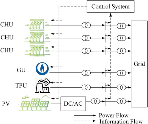
FIGURE 1. HTSGS structure diagram.

As shown in Figure 1, the CHUs consist of multiple cascade hydropower stations, which are connected to the power grid through transformers together with TPU and GU; In the PV power station, the PV array is connected to the power grid through the DC/AC inverter; The power generation control system collects and analyzes source data in real-time, and regulates the multiple sources. The power generation control system makes sure HTSGS can provide sufficient power side flexibility resources.

2.1 Model of flexible resources

2.1.1 Flexibility model of CHU

Compared with conventional TPU, CHU has the advantages of wide-range regulation and low cost. CHU is a good flexible resource. The maximum upward flexibility supply FSRup CHU(σ,t) and downward flexibility supply FSRdown CHU(σ,t) are provided by CHU as follows:

$FS{R}_{CHU}^{up}\left(\sigma ,t\right)=\min \left(RU\sigma ,P_{CHU}^{\mathit{max}}\left(t\right)-P_{CHU}\left(t\right)\right)(1)$

$FS{R}_{CHU}^{down}\left(\sigma ,t\right)=\min \left(RU\sigma ,P_{CHU}\left(t\right)-P_{CHU}^{\mathit{min}}\left(t\right)\right)(2)$

where σ is the time scale unit; RU and RD are the maximum and the minimum upward climbing rate of CHU; Pmax CHU and Pmin CHU are the maximum and minimum output of CHU at time t; P_CHU(t) is the actual output of CHU at time t.

2.1.2 Flexibility model of GU

The GU has the advantages of high-power generation efficiency and low pollution generation rate when operating under a high load rate. GU can also be used as a flexible resource to adjust the system operation performance.

The flexibility that GU can provide is defined as the maximum upward flexibility supply FSRup GU (σ,t) and downward supply FSRdown GU (σ,t):

$FS{R}_{GU}^{up}\left(\sigma ,t\right)=\min \left(R{U}_{\mathrm{g}}\sigma ,P_{GU}^{\mathit{max}}\left(t\right)-P_{GU}\left(t\right)\right)(3)$

$FS{R}_{GU}^{down}\left(\sigma ,t\right)=\min \left(R{D}_g\sigma ,P_{GU}\left(t\right)-P_{GU}^{\min }\left(t\right)\right)(4)$

where σ is the time scale unit; RU_g and RD_g are the maximum and the minimum upward climbing rate of GU; Pmax GU and Pmin GU are the maximum and minimum output of GU at time t; P_GU(t) is the actual output of GU at time t.

2.2 Model of flexible indexes

As shown in Figure 2, the green interval is the system reserve capacity range, the red curve is the system load curve, and the gray triangle with arrows represents the flexible scheduling output of the power system with HTSGS integration. Based on this, situation one shows that its gray triangle representing the system’s flexibility resources can only meet the lower limit of the system reserve capacity but cannot meet the upper limit, which means that the system is unable to balance the upward fluctuating load and the system has insufficient upward flexibility resources. Similarly, Situation two represents insufficient resources for the downward flexibility of the system. Situation three indicates that the system has sufficient upward and downward flexibility resources to balance the upward or downward fluctuation load. In this paper, the corresponding index model is developed to analyze the upward and downward flexibility resources.

FIGURE 2

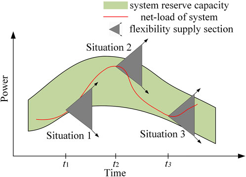
FIGURE 2. Schematic diagram of HTSGS flexibility evaluation.

2.2.1 Upward insufficient ramping resource probability

Upward insufficient ramping resource probability (UIRRP) η_UIRRP(t) is the probability that the flexibility provided by CHU and GU cannot meet the upward flexibility resource demand at time t when the power system with HTSGS integration operating, as shown in Eq. 5.

$\{\begin{array}{l}{\eta }_{UIRRP}\left(t\right)=\mathrm{Pr}\left\{{FSR}^{up}\left(t\right)-((P_{NL}(t+1)-(P_{NL}(t))<0\right\}\\ {FSR}^{up}\left(t\right)={FSR}_{CHU}^{up}\left(t\right)+{FSR}_{PSU}^{up}\left(t\right)\end{array}(5)$

where FSR^up(t) is the sum of the maximum upward flexibility supply provided by the system; P_NL(t) is the net-load of the system.

2.2.2 Downward insufficient ramping resource probability

Downward insufficient ramping resource probability (DIRRP) η_DIRRP(t) is the probability that the flexibility provided by CHU and GU cannot meet the downward flexibility resource demand at time t when the power system with HTSGS integration operating, as shown in Eq. 6.

$\{\begin{array}{l}{\eta }_{DIRRP}\left(t\right)=\mathrm{Pr}\left\{{FSR}^{down}\left(t\right)-((P_{NL}(t)-(P_{NL}(t+1))<0\right\}\\ {FSR}^{down}\left(t\right)={FSR}_{CHU}^{down}\left(t\right)+{FSR}_{PSU}^{down}\left(t\right)\end{array}(6)$

where FSR^down(t) is the sum of the maximum downward flexibility supply provided by the system.

2.2.3 Upward sufficient ramping resource expectation

Upward sufficient ramping resource expectation (USRRE) E_USRRE(t) is the expectation of the excess FSRM^up(t) that the upward flexibility resources provided by the HTSGS exceed the upward flexibility resources required by the system at time t during the power system operation, as shown in Eq. 7.

$\{\begin{array}{l}{E}_{USRRE}\left(t\right)={FSRM}^{up}\left(t\right)\cdot \mathrm{Pr}\{{FSR}^{up}\left(t\right)\\ -\left(P_{NL}\left(t+1\right)-P_{NL}\left(t\right)\right)>0\}\\ {FSRM}^{up}\left(t\right)={FSR}^{up}\left(t\right)-\left(P_{NL}\left(t+1\right)-P_{NL}\left(t\right)\right)\end{array}(7)$

2.2.4 Downward sufficient ramping resource expectation

Downward sufficient ramping resource expectation (DSRRE) E_DSRRE(t) is the expectation of the excess FSRM^down(t) that the downward flexibility resources provided by the HTSGS exceed the downward flexibility resources required by the system at time t during the power system operation, as shown in Eq. 8.

$\{\begin{array}{l}{E}_{DSRRE}\left(t\right)={FSRM}^{down}\left(t\right)\cdot \mathrm{Pr}\{{FSR}^{down}\left(t\right)\\ -\left(P_{NL}\left(t\right)-P_{NL}\left(t-1\right)\right)>0\}\\ {FSRM}^{down}\left(t\right)={FSR}^{down}\left(t\right)-\left(P_{NL}\left(t\right)-P_{NL}\left(t+1\right)\right)\end{array}(8)$

2.3 Modeling of DR

DR means that users can change their electricity consumption behavior through the change in electricity price, which can improve the power system operational flexibility. The elasticity coefficient of demand price indicates the relationship between the electricity load change and the electricity price change. The elasticity coefficient can be calculated as follows:

${\mu }_{nm}=\frac{∆L_n/{\lambda }_L{L}_{n0}}{∆Q_m/Q_{m0}}\{\begin{array}{l}{u}_{nm}\le 0,n=m\\ u_{nm}>0,n\ne m\end{array}(9)$

where ΔL_n0 and ΔQ_m are the electric load change and electricity price after DR; L_n0 and Q_m are load and electricity price before DR; λ_L is the adjustable load proportion in the electric load.

The change of electric load after DR within t periods can be expressed as:

$\left[\begin{array}{l}\frac{∆L_1}{L_1}\\ \frac{∆L_2}{L_2}\\ ⋮\\ \frac{∆L_t}{L_t}\end{array}\right]=\mu \left[\begin{array}{l}\frac{∆Q_1}{Q_1}\\ \frac{∆Q_2}{Q_2}\\ ⋮\\ \frac{∆Q_t}{Q_t}\end{array}\right](10)$

$\mu =\left[\begin{array}{cccc}{\mu }_{11}& {\mu }_{12}& \cdots & {\mu }_{1t}\\ {\mu }_{21}& {\mu }_{22}& \cdots & {\mu }_{2t}\\ ⋮& ⋮& ⋮& ⋮\\ {\mu }_{t1}& {\mu }_{t2}& \cdots & {\mu }_{tt}\end{array}\right](11)$

where μ is the price elasticity coefficient matrix of DR.

The DR model based on electricity price and load is established as follows:

$L_n=L_{n0}\left({\displaystyle \sum }_{m=1}^t\mu \frac{∆Q_m}{Q_{m0}}+\mu \frac{∆Q_n}{Q_{n0}}+1\right)(12)$

where L_n is the electric load after DR.

3 Economic scheduling model of power system with HTSGS

The objective function of the traditional economic scheduling model is to minimize the system operation cost. On this basis, this paper comprehensively considers the carbon emission reduction and the system flexibility guarantee and introduces the carbon emission cost and the risk cost of insufficient flexibility. A system economic scheduling model is built, and the multi-dimensional optimal coordinated scheduling of overall system operation economy, flexibility, and carbon emission reduction is realized.

3.1 System operation cost

The annual system operation cost consists of TPU operation cost C_TPU, CHU operation cost C_CHU and GU operation cost C_GU, as shown in Eq. 13.

$C_r=C_{TPU}+C_{CHU}+C_{GU}(13)$

The TPU operation cost includes the startup cost and unit cost of power generation, as shown in Eq. 14; CHU operation cost includes startup cost, shutdown cost, and flexibility cost, as shown in Eq. 15; GU operation cost includes the startup cost, shutdown cost, and gas cost, as shown in Eq. 16.

$C_{TPU}={\displaystyle \sum }_{t=1}^T{\displaystyle \sum }_{x=1}^{{\theta }_{TPU}}\left[c_x^{su}S{U}_x\left(t\right)+\left(a_x+b_x{P}_x\left(t\right)+c_x{P}_x{\left(t\right)}^2\right)\right](14)$

$C_{CHU}={\displaystyle \sum }_{t=1}^T{\displaystyle \sum }_{y=1}^{{\theta }_{CHU}}\left[c_y^{su}S{U}_y\left(t\right)+c_y^{sd}S{D}_y\left(t\right)+c_y^{op}{P}_y\left(t\right)\right](15)$

$C_{GU}={\displaystyle \sum }_{t=1}^T{\displaystyle \sum }_{z=1}^{{\theta }_{GU}}\left[\left[\begin{array}{l}{c}_z^{su}S{U}_z\left(t\right)+c_z^{sd}S{D}_z\left(t\right)+\\ \left(a_z{P}_z{\left(t\right)}^2+b_z{P}_z\left(t\right)+c_z\right)\end{array}\right]\right](16)$

Where T is the total number of scheduling periods; θ_TPU, θ_CHU and θ_GU are the set of TPU, CHU, GU; csu x is the startup cost of the xth TPU; a_x, b_x and c_x are the power generation cost coefficients of TPU; SU_x(t) is the 0–1 state variable to indicate xth TPU startup. When it is 0, the xth TPU is not started, and when it is 1, the TPU x is in the startup state; P_x(t) is the generating power of the TPU x at time t; csu y and csd yare the startup cost and shutdown cost of the yth CHU; SU_y(t) and SD_y(t) are 0–1 state variables for the startup and shutdown of the yth CHU; P_y(t) is the generating power of the yth CHU at time t; and cop y is the power generation cost coefficient of the yth CHU; csu z, csd z are the startup and shutdown costs of the zth GU; P_z(t) is the generating power of the zth GU at time t; a_z, b_z and c_z are the operating consumption coefficients of zth GU.

3.2 Carbon emission cost

The system purchases carbon emission rights in the carbon trading market according to carbon emission quotas and actual carbon emissions. The carbon emission quota allocation based on power generation is adopted in this paper. The carbon emission quota allocated to the system is approximately proportional to the total power generation of the system. The system carbon emission quota is as follows:

$E_D={\displaystyle \sum }_{t=1}^T\gamma P_a\left(t\right)(17)$

where E_D is the allocated carbon emission quota; γ is the carbon emission quota coefficient; P_a(t) is the total power generation of all generator units at time t.

In this paper, the carbon emissions of TPU and GU are considered. The actual carbon emission is as follows:

$E_C={\displaystyle \sum }_{t=1}^T{\displaystyle \sum }_{n=1}^{{\theta }_{TU}}{\eta }_n^{TU}{P}_n\left(t\right)+{\displaystyle \sum }_{t=1}^T{\displaystyle \sum }_{m=1}^{{\theta }_{GU}}{\eta }_m^{GU}{P}_m\left(t\right)(18)$

where E_C is the actual carbon emission of TPU and GU; P_n(t) and P_m(t) are the output power of the nth TPU and the mth GU at time t; ηTU n and ηGU m are the carbon emission coefficients of the nth TPU and the mth GU, respectively.

The carbon emission cost of this paper adopts the divided-interval ladder carbon trading model. The higher the carbon emission, the higher the carbon trading price required, as shown in Eq. 19.

$C_{co}=\{\begin{array}{l}\sigma \left(E_C-E_D\right)\\ E_C<E_D\\ \sigma \left(1+\mu \right)\left(E_C-E_D\right)\\ E_D\le E_D<E_D+\omega \\ \sigma \left(1+\mu \right)\omega +\sigma \left(1+\xi \mu \right)\left(E_C-E_D\right)\\ E_D+\omega \le E_C\end{array}(19)$

where σ Is the unit price of carbon trading; μ and ξ are the growth coefficients of carbon trading price, where ξ ≥ 2; ω is the corresponding carbon emission range.

3.3 System flexibility cost

The risk cost of insufficient flexibility includes the risk cost caused by insufficient upward flexibility and the risk cost caused by insufficient downward flexibility. It is determined by the multiplication of the upward and downward flexibility supply and demand difference and the risk cost coefficient of the corresponding lack of flexibility.

The upward flexibility resources shortage FSRS^up(t) is the difference between the upward flexibility demand and the actual upward flexibility supply capacity at time t.

${FSRS}^{up}\left(t\right)=\left(P_{NL}\left(t+1\right)-P_{NL}\left(t\right)\right)-{FSR}^{up}\left(t\right)(20)$

Similarly, the downward flexibility resources shortage FSRS^down(t) is the difference between the downward flexibility demand and the actual downward flexibility supply capacity at time t.

${FSRS}^{down}\left(t\right)=\left(P_{NL}\left(t\right)-P_{NL}\left(t+1\right)\right)-{FSR}^{down}\left(t\right)(21)$

Thus, the risk cost of insufficient flexibility C_FSRS is:

$C_{FSRS}={\displaystyle \sum }_{t\in T}({\lambda }_{up}{FSRS}^{up}(t)+{\lambda }_{down}{FSRS}^{down}(t))(22)$

where λ_up, λ_down are the risk cost coefficients that lack upward and downward flexibility.

3.4 Objective function

The minimum total cost C_a is taken as the objective function, and is composed of system operation cost C_r, carbon emission cost C_CO and risk cost of insufficient flexibility C_FSRS, as shown in Eq. 23.

$\min C_a=C_r+C_{co}+C_{FSRS}(23)$

3.5 Constraint conditions

3.5.1 Power flow constraint

The sum of the output of CHU, GU, and PV at any time during the whole scheduling period in the HTSGS should balance the system load. For any node b, the flexibility requirements for PV and load are as follows:

$\begin{array}{l}{\displaystyle \sum }_{x\in b}{P}_x\left(t\right)+{\displaystyle \sum }_{y\in b}{P}_y\left(t\right)+{\displaystyle \sum }_{z\in b}{P}_z\left(t\right)\\ +{\displaystyle \sum }_{l\in L_b}{P}_l\left(t\right)+{\displaystyle \sum }_{m\in b}{P}_{s,m}^{UL}\left(t\right)\ge {\displaystyle \sum }_{n\in b}{P}_{d,n}^{LL}\left(t\right)\end{array}(24)$

$\begin{array}{l}{\displaystyle \sum }_{x\in b}{P}_x\left(t\right)+{\displaystyle \sum }_{y\in b}{P}_y\left(t\right)+{\displaystyle \sum }_{z\in b}{P}_z\left(t\right)\\ +{\displaystyle \sum }_{l\in L_b}{P}_l\left(t\right)+{\displaystyle \sum }_{m\in b}{P}_{s,m}^{LL}\left(t\right)\le {\displaystyle \sum }_{n\in b}{P}_{d,n}^{UL}\left(t\right)\end{array}(25)$

where P_y(t) is the power generated by the CHU y at time t; P_z(t) is the power generated by the GU z at time t; l, L_b are the transmission line and the transmission line set of the corresponding node b; PUL s,m(t) and PLL s,m(t) are the upper and lower limits of the generated power of the PV m; PUL d,n(t) and PLL d,n(t) are the upper and lower limits of the load n.

Calculations and constraints for the DC power flow of the transmission line are as follows:

$P_l\left(t\right)=\frac{\left({\theta }_b\left(t\right)-{\theta }_{b^{\prime }}\left(t\right)\right)}{X_l}(26)$

$P_{l,\mathit{min}}\le P_l\left(t\right)\le P_{l,\mathit{max}}(27)$

where P_l(t) is the value of the transmission line power flow; P_l,max and P_l,min are the maximum and minimum power flow of the transmission line; X_l is the reactance of the transmission line l; θ_b is the phase angle of node b.

3.5.2 Operation constraints of TPU

The output constraint of TPU is as follows:

$P_{x,\min }\le P_x\left(t\right)\le P_{x,\max }(28)$

where P_x,min and P_x,max are the minimum and maximum output of the TPU x.

Ramping rate constraint of TPU is as follows:

$-R{U}_x∆t\le P_x\left(t\right)-P_x\left(t-1\right)\le R{D}_x∆t(29)$

where RU_x and RD_x are the upper and lower limits of the ramping rate of TPU x.

3.5.3 Operation constraints of CHU

The operation constraints of CHU include the upper and lower limits of storage capacity, power generation flow and discharge flow, water balance constraints, upper and lower output limits, and ramping constraints.

The upper and lower limits of storage capacity, power generation flow and discharge flow of CHU y are as follows:

$V_{y,\min }\le V_y\left(t\right)\le V_{y,\max }(30)$

$F_{y,\min }^{dc}\le F_y^{dc}\left(t\right)\le F_{y,\max }^{dc}(31)$

$F_{y,\min }^{out}\le F_y^{out}\left(t\right)\le F_{y,\max }^{out}(32)$

$F_y^{out}\left(t\right)=F_y^{fw}\left(t\right)+F_y^{dc}\left(t\right)(33)$

where V_y(t), V_y,min and V_y,max are the real-time, minimum and maximum storage capacity of the CHU y at time t; Fdc y(t), Fdc y, min and Fdc y, max are the real-time, minimum and maximum power generation flow of the CHU y at time t; Ffw y(t) and Fout y(t) are the waste and discharge water flow at time t; Fout y, min and Fout y, max are the minimum and maximum discharge water flow.

The water balance constraints of CHU are the change balance of the storage capacity of a single CHU over a certain time period and the change balance of the storage capacity of multiple CHUs in a certain space, as shown in Eq. 34 and Eq. 35.

$V_y\left(t+1\right)=V_y\left(t\right)+∆\tau ∆s\left(F_y^{in}\left(t\right)-F_y^{dc}\left(t\right)-F_y^{fw}\left(t\right)\right)(34)$

$F_y^{in}\left(t\right)=F_y^n\left(t\right)+{\displaystyle \sum }_{ur\in {\mathrm{\Omega }}_{URCHU}}\left(F_{ur}^{dc}\left(t\right)+F_{ur}^{fw}\left(t\right)\right)(35)$

where Fin y(t) is the water inflow of the CHU y at time t, Δs is the number of seconds per hour; Fn y(t) is the natural flow of the CHU y at time t; ur and Ω_URCHU are the number and number set of upstream CHUs.

The output of CHU shall be between the upper and lower limits of its output:

$P_{y,\min }\le P_y\left(t\right)\le P_{y,\max }(36)$

where P_y,min and P_y,max are the minimum and maximum output of CHU y.

The output of CHU is determined by the storage capacity and power generation flow:

$\begin{array}{l}{P}_y\left(t\right)=a_{1,y}{\left(V_y\left(t\right)\right)}^2+a_{2,y}{\left(F_y^{dc}\left(t\right)\right)}^2\\ +a_{3,y}{V}_y\left(t\right)F_y^{dc}\left(t\right)+a_{4,y}{V}_y\left(t\right)\\ +a_{5,y}{F}_y^{dc}\left(t\right)+a_{6,y}\end{array}(37)$

where a_1,y, a_2,y, a_3,y, a_4,y, a_5,y, a_6,y are the calculation coefficients of CHU output.

The difference between CHU output at time t and t+1 shall not exceed the maximum ramping output:

$\{\begin{array}{l}{P}_y\left(t+1\right)-P_y\left(t\right)\le \left(1-S{U}_y\left(t\right)\right)R{U}_y\\ P_y\left(t\right)-P_y\left(t+1\right)\le \left(1-S{D}_y\left(t\right)\right)R{D}_y\end{array}(38)$

where RU_y and RD_y are the maximum upward ramping output and maximum downward climbing output.

3.5.4 Operation constraints of GU

Operation constraints of GU include startup and shutdown constraints, output constraints, gas control constraints, and ramping rate constraints.

The increased times of GU startup and shutdown will shorten the GU’s service life and increase the startup and shutdown cost, so the upper limit of startup and shutdown times is taken as the operation constraint of GU.

${\displaystyle \sum }_{t=1}^T\left[S{U}_z\left(t\right)\cdot S{D}_z\left(t-1\right)\right]\le N_z(39)$

where N_z is the upper limit of the startup times of the GU z.

The output constraint of GU is as follows:

$P_{z,\min }\le P_z\left(t\right)\le P_{z,\max }(40)$

where P_z,min and P_z,max are the minimum and maximum output of the GU z.

In reality, the natural gas supply is still insufficient, so the daily power generation of GU is set as a constraint in scheduling as follows:

${\displaystyle \sum }_{t=1}^T{P}_z\left(t\right)\Delta t=E_z(41)$

where E_z is the daily power generation of GU z.

Ramping rate constraint of TPU is as follows:

$-R{U}_z\Delta t\le P_z\left(t\right)-P_z\left(t-1\right)\le R{D}_z\Delta t(42)$

where RU_z and RD_z are the upper and lower limits of the ramping rate of GU z.

3.5.5 Constraints of PV

The amount of radiation is the critical factor to determine the PV output power. The prediction error of radiation ΔR can be expressed as a normally distributed random variable with a mean of 0 and a standard deviation of σ_R. If the predicted value of radiation is R_P, the probability density function of the actual radiation R = R_P+ΔR is:

$f_R\left(R\right)=\frac{1}{\sqrt{2\pi }{\sigma }_R}{e}^{-{\left(R-R_P\right)}^2/2{{\sigma }_R}^2}(43)$

where the variance of the prediction error of the radiation is set to m% of the predicted value R_P.

The PV output power and radiation meet the relationships as follows:

$P_{PV}={\lambda }_{PV}R{S}_{PV}(44)$

where λ_PV is the conversion efficiency of PV power generation; S_PV is the total area of the PV array.

The PV output shall not exceed its upper limit.

$0<P_{PV}\le P_{PV,\max }(45)$

where P_PV,max is the maximum PV output.

3.5.6 Operation constraints of DR

Users participating in DR determine their own power load use according to the electricity price information. The total load used in the whole scheduling period remains unchanged and only changes in the power consumption time, that is, the change in the total load is 0, as shown in Eq. 46.

${\displaystyle \sum }_{t=1}^T\Delta L_m=0(46)$

After DR, the power consumption cost of users shall not exceed the power consumption cost before DR, as shown in Eq. 47.

${\displaystyle \sum }_{t=1}^T{Q}_n{L}_m\le {\displaystyle \sum }_{t=1}^T{Q}_{n0}{L}_{m0}(47)$

where Q_n0 and Q_n are the electricity price before and after DR.

3.5.7 Operational flexibility constraints

The upward and downward flexibility supply required by the power system with HTSGS integration is provided by the TPU, CHU, and GU, as shown in Eq. 48.

$\{\begin{array}{l}{FSR}^{up}\left(t\right)={\displaystyle \sum }_{x\in {\theta }_{TPU}}{FSR}_x^{up}\left(t\right)+{\displaystyle \sum }_{y\in {\theta }_{CHU}}{FSR}_y^{up}\\ +{\displaystyle \sum }_{z\in {\theta }_{GU}}{FSR}_z^{up}\left(t\right)\\ {FSR}^{down}\left(t\right)={\displaystyle \sum }_{x\in {\theta }_{TH}}{FSR}_x^{down}\left(t\right)+{\displaystyle \sum }_{y\in {\theta }_{CHU}}{FSR}_y^{down}\\ +{\displaystyle \sum }_{z\in {\theta }_{GU}}{FSR}_z^{down}\left(t\right)\end{array}(48)$

The flexibility supply provided by the TPU x at time t is constrained by the ramping rate and the upper and lower limits of output, as shown in Eq. 49.

$\{\begin{array}{l}{FSR}_x^{up}\left(t\right)\le \min \left(R{U}_x,P_{x,\max }-P_x\left(t\right)\right)\\ {FSR}_x^{down}\left(t\right)\le \min \left(R{D}_x,P_x\left(t\right)-P_{x,\min }\right)\end{array}(49)$

The flexibility supply provided by the CHU y at time t is also constrained by the ramping rate and the upper and lower limits of output, as shown in Eq. 50.

$\{\begin{array}{l}{FSR}_y^{up}\left(t\right)\le \min \left(R{U}_y,P_{y,\max }-P_y\left(t\right)\right)\\ {FSR}_y^{down}\left(t\right)\le \min \left(R{D}_y,P_y\left(t\right)-P_{y,\min }\right)\end{array}(50)$

The flexibility supply provided by the GU z at time t is also constrained by the ramping rate and the upper and lower limits of output, as shown in Eq. 51.

$\{\begin{array}{l}{FSR}_z^{up}\left(t\right)\le \min \left({RU}_z,P_{z,\max }-P_z\left(t\right)\right)\\ {FSR}_z^{down}\left(t\right)\le \min \left({RD}_z,P_z\left(t\right)-P_{z,\min }\right)\end{array}(51)$

4 Case studies

4.1 Parameters setting

The proposed model comprehensively considers the optimal utility of system flexibility index, carbon trading, and DR to the power system with HTSGS integration. The dispatcher can adjust the source and load on both sides according to the day-ahead load forecast results to minimize the total operation cost of the system. Then, a modified IEEE 30-bus system is used for case studies. The system includes 1 PV, 2 TPUs, 1 GU, and 3 CHUs. The location and technical parameters of each generator unit are shown in Table 1 and Figure 3. The model in this paper is a mixed integer linear programming model, which is globally optimized by calling the Yalmip/Gurobi commercial solver on Windows 7 computer (3.2 Ghz, 8GB, 4-core) under the MATLAB 2016 platform. The solution time is 24.73s, meeting the scheduling time requirement.

TABLE 1

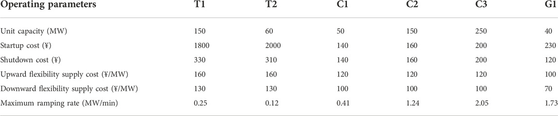
TABLE 1. Operating parameters of each unit.

FIGURE 3

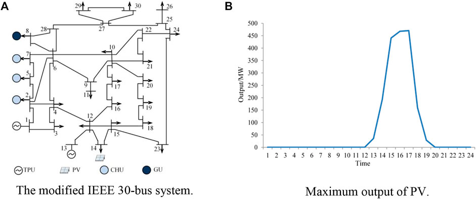
FIGURE 3. The location of each generator unit and maximum output of PV. (A) The modified IEEE 30-bus system. (B) Maximum output of PV.

To illustrate the advantages of the model proposed in this paper, four comparison scenarios are set as follows:

Scenario 1: system flexibility cost, carbon trading cost, and DR are considered at the same time;

Scenario 2: only the system carbon trading cost and DR are considered;

Scenario 3: only the system flexibility cost and carbon trading cost are considered;

Scenario 4: only the system flexibility cost and DR are considered.

4.2 Simulation results analysis

4.2.1 Comparison results based on flexibility indicators

This section will compare the scheduling results considering the system flexibility cost with those not considering the flexibility cost. The scheduling output sequence results are shown in Figures 4,5. It can be seen that in the scheduling scenario, without considering the flexibility cost, TPUs and CHUs mainly supply power. After considering the system flexibility, the GU keeps shut down at the time when the PV dominates the power supply at the source side, i.e., 3:00 pm-5:00 p.m. In contrast, the GU starts up at the time when the PV output is small, which significantly reduces the TPU output level. The power supply pressure of the CHUs is also alleviated. The above process considering flexibility cost reflects the flexible supply of the source side. In addition, the system’s PV abandonment rate is also reduced. This is because scenario one considers the flexibility limit of the system itself. By introducing the risk cost of insufficient flexibility into the objective function, the balance between the optimal economic cost and the reduction of the clean energy abandonment is achieved better.

FIGURE 4

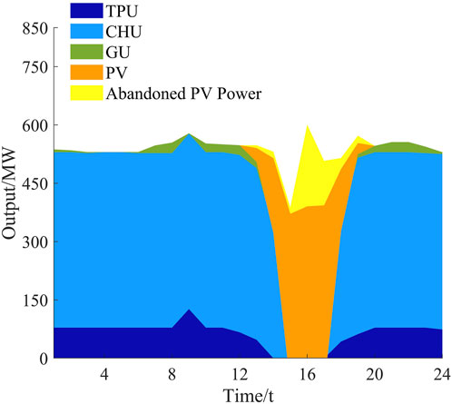
FIGURE 4. HTSGS scheduling results in Scenario 1.

FIGURE 5

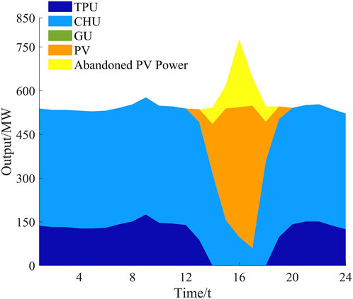
FIGURE 5. HTSGS scheduling results of in Scenario 2.

Scenario one is further refined to obtain the calculation results of the system flexibility index at all times over a day, as shown in Figures 6,7. Figure 6 corresponds to two upward flexibility indexes of UIRRP and USRRE; Figure 7 corresponds to the two downward flexibility indexes of DIRRP and DSRRE. It can be seen from Figures 6,7 that when it is between 2:00 p.m. and 6:00 p.m., the probability of insufficient system flexibility is 0. This is because the PV output is large during this period. The system can improve flexibility by switching the PV power station, and the sufficient system flexibility expectation is large. The maximum value of the USRRE index appears at 3:00 p.m., which is 15.73 MW, and the maximum value of the DSRRE index appears at 5:00 p.m., which is 9.02 MW. In contrast to the sufficient flexibility expectation index, the maximum values of insufficient flexibility probability and insufficient flexibility expectation appear at night, and the maximum values of UIRRP and UIRRE appear at 2:00 a.m., which are 8.48% and 19.20 MW, respectively; The maximum values of DIRRP and DIRRE indexes also appeared at 2:00 a.m., which are 5.51% and 5.23 MW, respectively. It can be seen that the system may still have insufficient flexibility at night. This provides data support for the system to plan further, invest and build high-quality flexible resources, and avoid PV abandonment caused by the imbalance between supply and demand of flexibility.

FIGURE 6

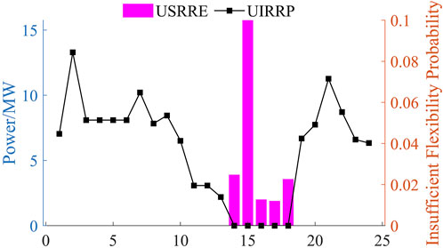
FIGURE 6. The USRRE&UIRRP results of HTSGS in Scenario 1.

FIGURE 7

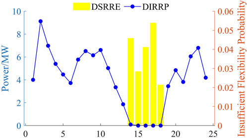
FIGURE 7. The DSRRE&DIRRP results of HTSGS in Scenario 1.

4.2.2 Comparison results of DR

The settings of scenario three and scenario one are mainly used to analyze the impact of DR implementation on system scheduling results. The scheduling output sequence results of scenario one have been given in the previous section. Here, the total load trend of the system with and without DR and the scheduling output sequence results of the units without DR are given, as shown in Figures 8, 9.

FIGURE 8

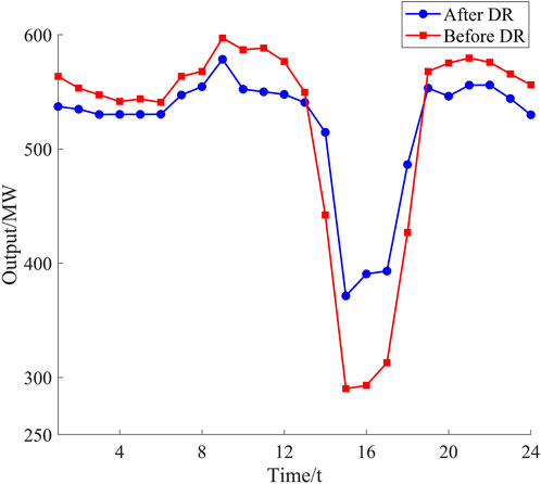
FIGURE 8. The total load comparison before and after DR.

FIGURE 9

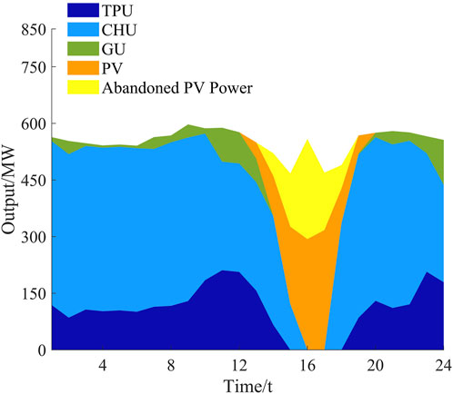
FIGURE 9. HTSGS Scheduling results in Scenario 3.

It can be seen that the overall trend of system scheduling output time sequence before and after DR implementation are similar, but there is a significant difference in output level. Specifically, since the cost of PV output is 0, the users participating in DR are stimulated to power consumption at 14:00–18:00, that is, the time when the PV output is large to reduce the system operation cost. The rest of the time, the power consumption of the system decreases, resulting in a decrease in TPU generation with the lowest output priority. However, due to system constraints, the total daily load remains unchanged. In general, the abandoned PV power is reduced after DR, which further verifies the technical advantages of DR implementation in promoting PV consumption.

4.2.3 Comparison results of carbon trading cost

The inclusion of carbon trading costs will lead to changes in the output of TPUs in the system, which will have a chain effect on the scheduling output of other units. Therefore, this paper sets scenarios one and four to make a comparative analysis on whether carbon trading cost is included. The scheduling output sequence results of scenario 4, which is not considering the carbon trading cost, are shown in Figure 10. It can be observed that the time series curve trend of system scheduling output is the same as that of scenario one considering carbon trading cost, but the TPU output level in scenario 4 has increased by about 50%. In addition, the output level of TPU in the early stage is relatively high, basically maintained at about 150 MW. When PV output is large, the abandoned PV power increases slightly due to an insufficient downward flexible supply of TPU itself.

FIGURE 10

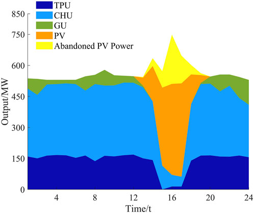
FIGURE 10. HTSGS Scheduling results in Scenario 4.

4.2.4 Economic and technical comparison of all scenarios

Table 2 illustrates the results of operation cost and abandoned PV power under different scenarios. Taking scenario 1 as a comparison benchmark, it can be seen that scenario two is not guided by the flexibility target, so its flexibility cost is significantly increased. Meanwhile, as its output is mainly generated by CHUs and TPUs, the power generation cost and carbon emission cost are also increased. Similarly, DR is not implemented in scenario 3, and the power generation cost rises by 12.8%, which fully reflects the economic deployment effectiveness deficiency in load following source side output. In scenario 4, because the carbon emission cost limit is ignored, the carbon emission cost increases by 31.37%, corresponding to the increase in the TPU output level. At the same time, the power generation cost in this scenario four also increases. Among the four scenarios, the total amount of abandoned PV power in scenario one is the lowest, which fully verifies the promotion effect on PV consumption of the scheduling model proposed in this paper.

TABLE 2

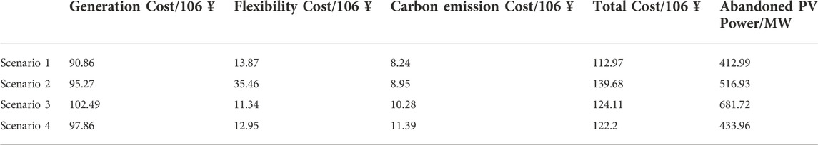
TABLE 2. The system costs and abandoned PV power among different scenarios.

4.2.5 Flexibility analysis under different power supply structures

To reveal the impact of different power constructures on system flexibility, the following four power constructive scenarios are set in this section:

Scenario 5: the system includes CHUs and GU;

Scenario 6: the system only includes CHUs, and other parameter settings are consistent;

Scenario 7: the system only includes GU, and the capacity of the original TPUs increases proportionally;

Scenario 8: the system does not include CHU and GU, and the capacity of the original TPUs increases proportionally.

The flexibility indexes of the system under different scenarios are shown in Table 3.

TABLE 3

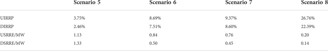
TABLE 3. The system flexibility results under different power source constructures.

It can be seen from Table 3 that the flexibility index UIRRP and DIRRP in scenario five is the smallest, which indicates that the power system under the HTSGS integration has the smallest probability of insufficient flexibility. In addition, the USRRE and DSRRE of scenario five reach 1.13 MW and 1.33MW, which indicates that the expectation of sufficient flexibility is high in scenario 5. Compared with scenario 5, the probabilities of insufficient flexibility are both increased in scenario six and scenario 7. The probability of insufficient flexibility in scenario eight reaches the maximum, where the UIRRP and DIRRP increase by 23.01% and 19.93% compared with scenario 5. In addition, the flexibility index USRRE and DSRRE are significantly reduced. This shows that when the HTSGS integration is not considered, the probability of insufficient power system flexibility is high, with 26.76% and 22.39% of probability of upward and downward insufficient flexibility. This is because the original TPUs of the system have the poor flexible regulation ability, and the flexible resource allocation of scenario eight is insufficient. From the above analysis, it can be seen that the HTSGS integration plays a positive role in improving the power system flexibility, which can effectively reduce the low flexibility probability and improve the sufficient flexibility probability of the system.

4.2.6 System economy analysis under different carbon trading prices

The carbon trading price will affect the system carbon cost, thus affecting the system scheduling results. This paper explores the operation cost and PV consumption rate under different carbon trading prices, and the results are shown in Figure 11.

FIGURE 11

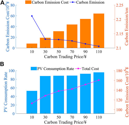
FIGURE 11. The economic and technical sensitivities at different carbon prices.

It can be seen that with the rise of carbon trading price, the PV consumption rate gradually rises, and the carbon emission continues to decline. However, the system’s carbon emission cost and total cost show an increasing trend. Among them, the carbon emission and PV consumption rate change obviously when the carbon emission price is among 10 and 30¥ and increases slowly after 30¥. At this time, the continued rise of carbon trading prices will bring little economic benefits to the system. In addition, due to the lower limit of TPU output, the PV consumption cannot be increased all the time, so the PV consumption trend slows down. In general, although the moderate increase in carbon emission price leads to an increase in system operation cost, the PV consumption rate and carbon emissions performances have been significantly improved, meeting the overall strategic requirements of energy conservation and emission reduction in the power industry.

5 Conclusion

In this paper, multi-dimensional economic scheduling is carried out for the power system with HTSGS integration considering its flexibility, carbon emission reduction, and DR. Firstly, the system flexibility resource is modeled, and the flexibility index is proposed. Then, considering the power flow constraints, source side operation constraints, system flexibility constraints, and DR constraints, a low-carbon flexible economic scheduling model of the system is constructed. The model minimizes the total cost of system operation, carbon emissions, and flexibility.

The case studies results show that the introduction of flexibility cost and carbon trading cost is beneficial to the system to adjust the scheduling strategy and reduce the PV power abandonment; DR can improve the source load timing balance and promote PV consumption. In general, the comprehensive consideration of system flexibility cost, carbon trading cost, and DR can effectively reduce system cost, improve system flexibility, and reduce carbon emission.

The internal multiple sources of HTSGS can complement each other and promote PV consumption. In addition, the sufficient flexibility of the system has been significantly improved after the HTSGS integration.

The system’s carbon emissions will significantly decrease with the increase of the carbon trading price within a certain limit, and the PV consumption rate and the carbon emission price show the same trend.

In future work, we can study the effect of various renewable energy power generation scenarios, i.e., different weather conditions, on the proposed scheduling model. Besides, establishing a robust economic optimization scheduling model by fully considering the relationship between the robustness and economic constraints of the proposed scheduling strategy is worth studying. (Bouffard and Ortega-Vazquez, 2011), (Lannoye et al., 2012)., (Menemenlis et al., 2011).

Data availability statement

The raw data supporting the conclusions of this article will be made available by the authors, without undue reservation.

Author contributions

All authors have made substantial contributions to the conception, design of the work; analysis; and drafting of the paper. All authors read and approved the final manuscript.

Funding

This research is supported by the Science and Technology Project of State Grid Corporation of China (Grant No. 5108-202226031A-1-1-ZN). The funder was not involved in the study design, collection, analysis, interpretation of data, the writing of this article, or the decision to submit it for publication.

Conflict of interest

Authors DZ, YW, LX, FD, and ZD was employed by the State Grid Sichuan Electric Power Company.

The remaining authors declare that the research was conducted in the absence of any commercial or financial relationships that could be construed as a potential conflict of interest.

Publisher’s note

All claims expressed in this article are solely those of the authors and do not necessarily represent those of their affiliated organizations, or those of the publisher, the editors and the reviewers. Any product that may be evaluated in this article, or claim that may be made by its manufacturer, is not guaranteed or endorsed by the publisher.

References

Akbari-Dibavar, A., Mohammadi-Ivatloo, B., Zare, K., Khalili, T., and Bidram, A. (2021). Economic-emission dispatch problem in power systems with carbon capture power plants. IEEE Trans. Ind. Appl. 57 (4), 3341–3351. doi:10.1109/tia.2021.3079329

CrossRef Full Text | Google Scholar

Bouffard, F., and Ortega-Vazquez, M. (July 2011). "The value of operational flexibility in power systems with significant wind power generation", Proceedings of the 2011 IEEE Power and Energy Society General Meeting, Detroit, MI, USA, 1–5.

Google Scholar

Brahma, D., and Senroy, N. (2020). Sensitivity-based approach for assessment of dynamic locational grid flexibility. IEEE Trans. Power Syst. 35 (5), 3470–3480. doi:10.1109/tpwrs.2020.2985784

CrossRef Full Text | Google Scholar

Buhan, S., Kucuk, D., Cinar, M. S., Guvengir, U., Demirci, T., Yilmaz, Y., et al. (2020). A scalable river flow forecast and basin optimization system for hydropower plants. IEEE Trans. Sustain. Energy 11 (4), 2220–2229. doi:10.1109/tste.2019.2952450

CrossRef Full Text | Google Scholar

Du, E., Zhang, N., Hodge, B.-M., Wang, Q., Lu, Z., Kang, C., et al. (2019). Operation of a high renewable penetrated power system with CSP plants: A look-ahead stochastic unit commitment model. IEEE Trans. Power Syst. 34 (1), 140–151. doi:10.1109/tpwrs.2018.2866486

CrossRef Full Text | Google Scholar

Emmanuel, M., Doubleday, K., Cakir, B., Marković, M., and Hodge, B.-M. (2020). A review of power system planning and operational models for flexibility assessment in high solar energy penetration scenarios. Sol. Energy 210, 169–180. doi:10.1016/j.solener.2020.07.017

CrossRef Full Text | Google Scholar

Fan, L., Zhao, C., Zhang, G., and Huang, Q. (2022). Flexibility management in economic dispatch with dynamic automatic generation control. IEEE Trans. Power Syst. 37 (2), 876–886. doi:10.1109/tpwrs.2021.3103128

CrossRef Full Text | Google Scholar

Heggarty, T., Bourmaud, J.-Y., Girard, R., and Kariniotakis, G. (2020). Quantifying power system flexibility provision. Appl. Energy 279, 115852. doi:10.1016/j.apenergy.2020.115852

CrossRef Full Text | Google Scholar

Lannoye, E., Flynn, D., and O'Malley, M. (2012). Evaluation of power system flexibility. IEEE Trans. Power Syst. 27 (2), 922–931. doi:10.1109/tpwrs.2011.2177280

CrossRef Full Text | Google Scholar

Li, H., Zhang, N., Fan, Y., Dong, L., and Cai, P. (2022). Decomposed modeling of controllable and uncontrollable components in power systems with high penetration of renewable energies. J. Mod. Power Syst. Clean Energy 10 (5), 1164–1173. doi:10.35833/mpce.2020.000674

CrossRef Full Text | Google Scholar

Li, P., Yu, D., Yang, M., and Wang, J. (2018). Flexible look-ahead dispatch realized by robust optimization considering CVaR of wind power. IEEE Trans. Power Syst. 33 (5), 5330–5340. doi:10.1109/tpwrs.2018.2809431

CrossRef Full Text | Google Scholar

Lu, Z., Li, H., and Qiao, Y. (2018). Probabilistic flexibility evaluation for power system planning considering its association with renewable power curtailment. IEEE Trans. Power Syst. 33 (3), 3285–3295. doi:10.1109/tpwrs.2018.2810091

CrossRef Full Text | Google Scholar

Ma, J., Silva, V., Belhomme, R., Kirschen, D. S., and Ochoa, L. F. (2013). Evaluating and planning flexibility in sustainable power systems. IEEE Trans. Sustain. Energy 4 (1), 200–209. doi:10.1109/tste.2012.2212471

CrossRef Full Text | Google Scholar

Ma, R., Li, K., Li, X., and Qin, Z. (2015). An economic and low-carbon day-ahead Pareto-optimal scheduling for wind farm integrated power systems with demand response. J. Mod. Power Syst. Clean. Energy 3 (3), 393–401. doi:10.1007/s40565-014-0094-7

CrossRef Full Text | Google Scholar

Menemenlis, N., Huneault, M., and Robitaille, A. (July 2011). "Thoughts on power system flexibility quantification for the short-term horizon", Proceedings of the 2011 IEEE Power and Energy Society General Meeting, Detroit, MI, USA, 1–8.

Google Scholar

Mohandes, B., Moursi, M. S. E., Hatziargyriou, N., and Khatib, S. E. (2019). A review of power system flexibility with high penetration of renewables. IEEE Trans. Power Syst. 34 (4), 3140–3155. doi:10.1109/tpwrs.2019.2897727

CrossRef Full Text | Google Scholar

Reddy, S. K., Panwar, L. K., Panigrahi, B. K., and Kumar, R. (2017). Modeling of carbon capture technology attributes for unit commitment in emission-constrained environment. IEEE Trans. Power Syst. 32 (1), 662–671. doi:10.1109/tpwrs.2016.2558679

CrossRef Full Text | Google Scholar

Shi, Y., Dong, S., Guo, C., Chen, Z., and Wang, L. (2021). Enhancing the flexibility of storage integrated power system by multi-stage robust dispatch. IEEE Trans. Power Syst. 36 (3), 2314–2322. doi:10.1109/tpwrs.2020.3031324

CrossRef Full Text | Google Scholar

Wang, S., Liu, J., Chen, H., Bo, R., and Chen, Y. (2021). Modeling state transition and head-dependent efficiency curve for pumped storage hydro in look-ahead dispatch. IEEE Trans. Power Syst. 36 (6), 5396–5407. doi:10.1109/tpwrs.2021.3084909

CrossRef Full Text | Google Scholar

Wang, Y., Qiu, J., and Tao, Y. (2022). Optimal power scheduling using data-driven carbon emission flow modelling for carbon intensity control. IEEE Trans. Power Syst. 37 (4), 2894–2905. doi:10.1109/tpwrs.2021.3126701

CrossRef Full Text | Google Scholar

Yamujala, S., Kushwaha, P., Jain, A., Bhakar, R., Wu, J., and Mathur, J. (2021). A stochastic multi-interval scheduling framework to quantify operational flexibility in low carbon power systems. Appl. Energy 304, 117763. doi:10.1016/j.apenergy.2021.117763

CrossRef Full Text | Google Scholar

Zhang, S., Xiang, Y., Liu, J., Liu, J., Zhao, X., Jawad, S., et al. (2022). A regulating capacity determination method for pumped storage hydropower to restrain PV generation fluctuation. CSEE J. Power Energy Syst. 8 (1), 304–316. doi:10.17775/cseejpes.2020.01930

CrossRef Full Text | Google Scholar

Zhao, J., and Xu, Z. (2017). Ramp-limited optimal dispatch strategy for PV-embedded microgrid. IEEE Trans. Power Syst. 32 (5), 4155–4157. doi:10.1109/tpwrs.2017.2670920

CrossRef Full Text | Google Scholar

Zhao, Y., Wang, C., Zhang, Z., and Lv, H. (2021). Flexibility evaluation method of power system considering the impact of multi-energy coupling. IEEE Trans. Ind. Appl. 57 (6), 5687–5697. doi:10.1109/tia.2021.3110458

CrossRef Full Text | Google Scholar