Optimization of photovoltaic panel deployment in centralized photovoltaic power plant under multiple factors

1 Introduction

Rapid development of renewable energy technologies such as solar is required due to climate change mitigation strategies worldwide (Dong et al., 2021). Moreover, the development of photovoltaic (PV) power technologies plays an important role in achieving the goals of emission peak and carbon neutrality (Zhang et al., 2021), and poverty alleviation (Zhang et al., 2020). However, the performance of PV systems is generally affected by the meteorological conditions (Hachicha et al., 2019; Li et al., 2021), and geographical location (Al-Rousan et al., 2018; Cotfas and Cotfas, 2019). Furthermore, the centralized PV power plant covers a large area, and its continuous expansion also causes the problem of insufficient land. Therefore, it is necessary to make full use of the meteorological and geographical conditions in different regions to develop PV.

Different meteorological factors effect on PV output power to different extent. Therefore, the first step of centralized PV plant planning is to start with the effect caused by meteorological factors. Mekhilef et al. (2012) studied the effect of dust deposition, wind speed and relative humidity on the efficiency of solar cells. Li et al. (2020) analyzed the impacts of wind speed, wind direction, ambient temperature and solar radiation on PV considering dynamic line parameters. The main factors in the PV power calculation are the solar insolation. Ambient temperature and wind speed have transitive relation with PV power through irradiance, and the humidity and the atmospheric pressure have a negative correlation with PV output (Ziane et al., 2021). Dust is a cause of PV output power reduction, and models of dust deposition on PV modules using local meteorological events were developed in (Sengupta et al., 2021). Gowid and Massoud (2020) developed a PV maximum power point identification tool considering temperature and solar insolation. Mayer (2021) revealed the effects of the meteorological data resolution on the of simulation and optimization reliability of PV power plants. Those studies points out what and how meteorological factors affect PV output power, but most of them did not consider enough kinds of meteorological factors.

After confirming what and how meteorological factors affect the PV output power, PV output power calculation or prediction based on multiple meteorological factors has become a hot topic in recent years. Correlation analysis and regression analysis are basic methods to calculate PV power. A model of PV output power was obtained through regression analysis by selecting main factors that affect PV power in (Kim et al., 2019). Agoua et al. (2018) proposed a statistical spatio-temporal model based on correlation analysis to improve short-term forecasting of PV production. However, the methods mentioned above have relatively low efficiency and accuracy. To overcome this problem, a widely-used kind of method for PV calculation or prediction is deep learning. Considering solar radiation, sunlight, wind speed, temperature, cloud cover, and humidity, a modified long short-term memory (LSTM) is used to predict PV power in medium and long term (Son and Jung, 2020). There are also many other deep learning based methods such as methods based on convolutional neural network (Yan et al., 2021), spatiotemporal feedforward neural network (Rodríguez et al., 2022) and so on. Besides, graph modeling method is a novel method for PV power prediction. The graph modeling method is used to describe the relationship between various meteorological factors and PV power and predict the PV power, but the graph modeling method is more complex (Cheng et al., 2021). There are already various practical PV calculation methods taking meteorological factors into account, but there are few studies considering geographical conditions which also affect PV output power. To sum up, the method for PV output power calculation still needs to develop.

As mentioned above, the performance of PV is also affected by geographical conditions. For example, according to a study in a water pumping system with PV installation in Brazil, when the ratio between flow and radiation was taken into account, the monocrystalline PV system was more efficient (Nogueira et al., 2015). Polycrystalline solar module showed a better performance in semi-arid Region (Ettah et al., 2021). Ingenhoven et al. (2019) analyzed the performance loss rate of six different PV module types in five locations in Italy. Huld (2017) promoted a set of tool and data named PVMAPS, which could calculate PV performance in any region covered by the data. Due to the relationship between geographical conditions and PV performance, site selection became an important factor of PV power plant execution. To find the best location, many researches presented methods based on geographical information system (Hashemizadeh et al., 2019; Mensour et al., 2019). Although some literature dealt with the site selection of PV power plant, there were not many literature focus on the deployment of PV panels in centralized PV power plant.

In summary, the existing works lack an optimization method for the deployment of PV panels in a centralized PV power plant considering not only the geographical difference but the meteorological difference. To solve the above problems, this paper proposes an optimization method for the deployment of PV panels in a centralized PV power plant considering multiple factors. By optimizing the deployment position and quantity of PV panels, the method aims at higher PV output power and lower cost under certain capacity and approximate planning area for a centralized PV power plant. It also provides possibility for more efficient application of PV.

The remainder of the paper is organized as follows. Section 2 introduces terrain clustering, quantification of the relationship between meteorological factors and PV output, and optimization model. Section 3 shows the result of case studies. Section 4 makes a conclusion for this paper.

2 Methodologies

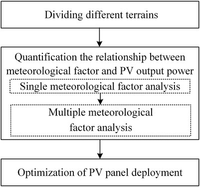
As shown in Figure 1, the method for optimizing the deployment of PV panels in a centralized PV power plant under multiple factors is divided into three steps: dividing different terrains in the PV power plant according to geographical characteristics, modeling and quantifying the relationship between meteorological factors and PV output power in each terrain (including single meteorological factor and multiple meteorological factor analysis), optimizing the deployment of PV panels in the centralized PV power plant.

FIGURE 1

FIGURE 1. Three steps of the method for deployment of PV panels.

2.1 Terrain clustering

Before studying meteorological factors, we should first explore the influence of geographical factors. This is because the meteorological conditions in different locations are obviously different. Thus, to carefully study the relationship among PV output power, meteorological factors and geographical factors, it is necessary to combine the sub-areas with similar geographical locations to a terrain first. Moreover, the installation of PV panels is also affected by geographical factors. For example, according to the different slope direction and gradient, the installation area of unit PV panels varies, and the unit installation area will affect the subsequent optimal deployment of PV panels. Therefore, based on the above considerations, this section first divides the surrounding area of a planned centralized PV power station into several terrains according to the geographical characteristics.

Noted that the PV panels in a centralized PV power plant are often orderly concentrated in a certain area, the distance and direction between the terrain center and the gathering station (GS) are included in the geographical characteristics, so as to make each sub-area within the divided terrain roughly similar in location and more accord with the actual situation of the centralized PV power plant construction. Firstly, PV power plant are divided into several sub-areas from west to east and from north to south according to a rectangular area with the same area of A_N (determined according to the actual cases). Then the annual sunshine durations, average altitude, slope direction, slope, distance between the terrain center and the GS, the direction of the terrain center relative to the GS are used as the geographical features for dividing different terrains. Define the geographical feature of the ith sub-area as $X_i^{terrain}$ and establish the dataset $X_i^{terrain}=\left\{x_{i1}^{terrain},x_{i2}^{terrain},\cdots ,x_{i6}^{terrain}\right\}$. Subscripts i1 to i6 represent the annual sunshine durations, average altitude, slope direction, slope, distance between the terrain center and the GS, the direction of the terrain center relative to the GS in the ith sub-area, respectively.

As one of the main unsupervised machine learning technologies, fuzzy clustering analysis is a method of analyzing and modeling important data using fuzzy theory, which establishes the uncertainty description of sample categories. The vector of fuzzy clustering algorithm can belong to multiple clusters at the same time, which can objectively reflect the real world. It has been effectively applied in many fields such as large-scale data analysis, data mining, vector quantization and so on, which is proved to have important theoretical and practical application value. With the further development of application, the research of fuzzy clustering algorithm is constantly enriched. In this section, we have chosen fuzzy c-means (FCM) algorithms due to its good performance (Benmouiza et al., 2016), and the FCM algorithm introduced by Dunn and improved by Bezdek (Nayak et al., 2015).

Using the FCM algorithm, a total of K sub-areas in the whole planning area of the PV power plant are classified into N terrains. The idea of FCM algorithm is to calculate the membership matrix $U={\left[u_{ij}\right]}_{N\times K}$ and the cluster centers $V=\left\{v_1,v_2,\cdots ,v_N\right\}$ from the terrain geographic feature dataset $X^{terrain}=\left\{X_1^{terrain},X_2^{terrain},\cdots ,X_K^{terrain}\right\}$ through continuous iteration, and to minimize the function value in Eq. 1.

$J\left(U,V\right)={\displaystyle \sum }_{i=1}^K{\displaystyle \sum }_{j=1}^N{u}_{ij}^m{d}_{ij}^2(1)$

$d_{ij}=‖X_i^{terrain}-v_j‖(2)$

In Eq. 1, u_ij is the membership degree of the ith sub-area belonging to the jth terrain; m is the membership factor; d_ij is the Euclidean distance from the ith sub-area to the jth cluster center, which is calculated by Eq. 2.

The calculation steps of the FCM algorithm are as follows:

Step 1. N cluster centers are randomly selected and the initial membership matrix U⁽⁰⁾ is calculated. Let l = 1 and start the first iteration.

Step 2. Calculate the cluster center V^(l) and membership matrix U^(l) of the lth iteration, and calculate the function value of J^(l), as shown in follows.

$v_j^{\left(l\right)}=\frac{{\displaystyle \sum }_{i=1}^K{\left(u_{ij}^{\left(l-1\right)}\right)}^m{X}_i^{terrain}}{{\displaystyle \sum }_{i=1}^K{\left(u_{ij}^{\left(l-1\right)}\right)}^m},j=\mathrm{1,2},\cdots ,N(3)$

$u_{ij}^{\left(l\right)}=\frac{1}{{\displaystyle \sum }_{i=1}^K{\left(\frac{d_{ij}^{\left(l\right)}}{d_{ik}^{\left(l\right)}}\right)}^{\frac{2}{m-1}}},i=\mathrm{1,2},\cdots K;j=\mathrm{1,2},\cdots ,N(4)$

$J^{\left(l\right)}\left(U^{\left(l\right)},V^{\left(l\right)}\right)={\displaystyle \sum }_{i=1}^K{\displaystyle \sum }_{j=1}^N{\left({\left(u\right)}_{ij}^{\left(l\right)}\right)}^m{\left({\left(d\right)}_{ij}^{\left(l\right)}\right)}^2(5)$

$d_{ij}^{\left(l\right)}=‖X_i^{terrain}-v_j^{\left(l\right)}‖(6)$

Step 3. Set the termination value. Membership termination value ε_u > 0 or function termination value ε_J > 0 can be used. If $\max \left\{\left|u_{ij}^{\left(l\right)}-u_{ij}^{\left(l-1\right)}\right|\right\}<{\epsilon }_u$ or $\left|J^{\left(l\right)}-J^{\left(l-1\right)}\right|<{\epsilon }_J$, the iteration stops, otherwise, increase l and go to step 2.When $u_{ij}={\mathit{max}}_{1\le j\le N}\left\{u_{ij}\right\}$, the ith sub-area belongs to the jth terrain and can be expressed as follows:

$X_i^{terrain}\in D_j(7)$

2.2 Single meteorological factor analysis

Quantification the relationships between meteorological factors and PV output power in each terrain includes single meteorological factor and multiple meteorological factor analysis. There are many kinds of meteorological factors, and the impact of various meteorological factors on PV output power may be significantly different. Therefore, in order to accurately measure the relationship between meteorological factors and PV output power, and simplify the calculation complexity and time of subsequent multiple meteorological factors analysis without losing accuracy, a single meteorological factor analysis of PV output power is conducted first. The single meteorological factor analysis is to select the daily output data of an existing PV power plant near the planning area and various meteorological data collected by the corresponding meteorological station as historical data, preliminarily analyze the relationships between PV output power and various meteorological factors through Pearson correlation coefficient, and select several major meteorological factors that have a great impact on the PV output.

$r=\frac{{\displaystyle \sum }_{i=1}^n\left(x_i-\overline{x}\right)\left(y_i-\overline{y}\right)}{\sqrt{{\displaystyle \sum }_{i=1}^n{\left(x_i-\overline{x}\right)}^2·{\displaystyle \sum }_{i=1}^n{\left(y_i-\overline{y}\right)}^2}}(8)$

$\overline{x}=\frac{1}{n}{\displaystyle \sum }_{i=1}^n{x}_i(9)$

$\overline{y}=\frac{1}{n}{\displaystyle \sum }_{i=1}^n{y}_i(10)$

Where x_i is the ith time component of the meteorological factor x, y_i is the ith time component of PV output y, r is the correlation coefficient, r∈[−1,1], and the closer the absolute value is to 1, the stronger the correlation between the meteorological factor x and PV output.

According to the value of correlation coefficient, k meteorological factors with the strongest correlation with PV output are selected for further mining the relationship between meteorological factors and PV output. Considering that the dimensions of various meteorological factors and PV output are not uniform, the MinMaxScaler method is used to normalize the data to improve the convergence speed of the subsequent deep learning model and reduce the error. MinMaxScaler method is shown in Eq. 11:

$x^{\prime }=\frac{x-x_{\mathit{min}}}{x_{\mathit{max}}-x_{\mathit{min}}}(11)$

where, $x^{\prime }$ is the normalized data, x is the original data, x_min and x_max are the minimum and maximum of the original data.

After normalizing the k main meteorological factors and PV output data, sequential feature $X^{me}=\left(x_1^{me},x_2^{me},\cdots ,x_T^{me}\right)={\left(x^{me1},x^{me2},\cdots ,x^{mek}\right)}^T$, containing k main meteorological factors, is constructed. It can be expressed by the following matrix:

$X^{me}=\left[\begin{array}{cc}\begin{array}{c}\begin{array}{cc}{x}_1^{me1}& x_1^{me2}\\ x_2^{me1}& x_2^{me2}\end{array}\\ \begin{array}{cc}⋮& ⋮\\ x_T^{me1}& x_T^{me2}\end{array}\end{array}& \begin{array}{c}\begin{array}{cc}\cdots & x_1^{mek}\\ \cdots & x_2^{mek}\end{array}\\ \begin{array}{cc}\ddots & ⋮\\ \cdots & x_T^{mek}\end{array}\end{array}\end{array}\right](12)$

where, $x_t^{me}=\left(x_t^{me1},x_t^{me2},\cdots ,x_t^{mek}\right)$ is expressed as the above k meteorological feature sets at time t, and $x^{mep}=\left(x_1^{mep},x_2^{mep},\cdots ,x_T^{mep}\right)$ is expressed as the each value of the pth relevant meteorological variable for the whole period T.

2.3 Multiple meteorological factor analysis

The multiple meteorological factor analysis uses the dual-stage attention mechanism based LSTM (DA-LSTM). LSTM is an improved recurrent neural network. Each hidden layer is no longer a single neural network, but consists of four interconnected neural networks (forget gate, input gate, update gate and output gate). It compares the memory information with the current information and learns through self-evaluation and selectively forgetting mechanism, which can alleviate the problem of gradient vanishing and exploding in general recurrent neural network (Greff et al., 2017; Shewalkar, 2019).

2.3.1 Overview of long short-term memory

In the general LSTM networks, the long-term memory information at time t is defined as the cell state C_t. The LSTM cell receives the meteorological feature set $x_t^{me}$ at time t and the short-term memory information h_t-1 of cells at the previous time, and inputs the cell state C_t-1 at the previous time into each gate as internal information. Through the forget gate f_t, the input gate i_t and the output gate o_t, the cell information is read and modified as follows:

$f_t=\sigma \left(W_f·\left[h_{t-1},x_t^{me}\right]+b_f\right)(13)$

$i_t=\sigma \left(W_i·\left[h_{t-1},x_t^{me}\right]+b_i\right)(14)$

$C_t^{\prime }=\mathit{tanh}\left(W_C·\left[h_{t-1},x_t^{me}\right]+b_C\right)(15)$

$o_t=\sigma \left(W_o·\left[h_{t-1},x_t^{me}\right]+b_o\right)(16)$

where, W_f, W_i and W_o are the weight matrices of forget gate, input gate and output gate respectively, and b_f, b_i and b_o are the corresponding biases. W_C is the input cell state weight matrix, and b_C is the bias of the input cell state. σ is the sigmoid activation function, which transforms the output into [0,1] interval, tanh is a hyperbolic tangent activation function, which transforms the output into the [−1,1] interval. Eq. 13 represents a forget gate for judging whether the previous information is retained. Eq. 14 represents an input gate that determines whether the current information is written to the cell state at time t; Eq. 15 creates a new vector containing all possible values through the tanh activation function and adds it to the cell state; Eq. 16 represents an output gate that determines the information to be included in the output content. Input the hidden layer output h_t to obtain the PV output y_t, and the calculation is as shown in Eqs. 17–19.

$C_t={f_t*C_{t-1}+i_t*C}_t^{\prime }(17)$

$h_t=o_t*\mathit{tanh}\left(C_t\right)(18)$

$y_t=W_d{h}_t+b_d(19)$

where, * denotes the multiplication of matrix elements. W_d and B_d are the adjustable weight matrix and the bias of the output layer, respectively.

2.3.2 Dual-stage attention

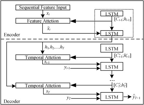
The performance of only using ordinary LSTM under sudden weather and extreme weather conditions is often poor, so the attention mechanism is introduced. The attention mechanism imitates how the human brain processes information, which improves the performance of the neural network (Qu et al., 2021). In this paper, the feature attention mechanism is introduced at the encoder side, and the time attention mechanism is introduced at the decoder side to build a dual-stage attention mechanism, so as to obtain a more accurate relationship between PV output power and meteorological factors and historical information. The dual-stage attention structure can be shown in Figure 2.

FIGURE 2

FIGURE 2. The structure of DA-LSTM.

Feature attention models the importance of each feature and assigns different attention to each dimension of the input (Zeng et al., 2022). In order to obtain the contribution rate of each meteorological feature to the PV output at the current time, the relevant meteorological features at time t are input into the feature attention mechanism to obtain the attention weight vector e_t:

$e_t=V_e^T\mathit{tanh}\left(W_e\left[h_{t-1},C_{t-1}\right]+U_e{x}^{mep}+b_e\right)(20)$

where, $e_t=\left(e_t^1,e_t^2,\cdots ,e_t^k\right)$ is the combination of attention weight coefficients corresponding to each meteorological feature at time t; V_e, W_e and U_e are the weight matrix of attention mechanism, and b_e is the bias. Normalization is performed according to Eq. 21, using the Softmax function so that the sum of the feature attention weights is 1. The normalized feature attention weight is expressed as ${\alpha }_t=\left({\alpha }_t^1,{\alpha }_t^2,\cdots ,{\alpha }_t^p,\cdots ,{\alpha }_t^k\right)$, where ${\alpha }_t^p$ is the feature attention weight value of the pth relevant meteorological feature at time t.

${\alpha }_t^p=\frac{\mathit{exp}\left(e_t^p\right)}{{\displaystyle \sum }_{i=1}^k\mathit{exp}\left(e_t^i\right)}(21)$

Multiplying the feature attention weight value ${\alpha }_t^p$ with the corresponding meteorological feature value $x_t^{mep}$ to obtain the correlation feature ${\stackrel{\sim }{x}}_t^{mep}$ considering the contribution rate of different meteorological features:

${\stackrel{\sim }{x}}_t=\left({\alpha }_t^1{x}_t^{me1},{\alpha }_t^2{x}_t^{me2},\cdots ,{\alpha }_t^k{x}_t^{mek}\right)(22)$

By introducing the feature attention mechanism, the input to the LSTM network is no longer the original meteorological feature value, but the correlation feature weighted by the contribution rate. It adaptively strengthens the key factors affecting the PV output, weakens the less relevant meteorological factors, and improves the modeling accuracy.

Temporal attention mechanism is introduced for finding the characters of trend and cycle and determining the key node for the current PV output power adaptively (Zhu et al., 2022). In order to obtain the contribution rate of the sequential state in a period of time on the PV output at the current time, obtain the weight of the hidden state of the corresponding time sequence, and extract the historical key node, introduce the temporal attention mechanism at the decoding output side. The temporal attention weightof the hidden layer state at the current time depends on the hidden layer state $h_t=\left(h_t^1,h_t^2,\cdots ,h_t^T\right)$ of the selected historical time sequence of LSTM, T is the time length of the input sequence. Taking it as an input, the temporal attention weight coefficient $l_t=\left(l_t^1,l_t^2,\cdots ,l_t^{\tau },\cdots ,l_t^T\right)$ at the current time t is obtained, as shown in the Eq. 23:

$l_t^{\tau }=V_d^T\mathit{tanh}\left(W_d[h_{t-1}^{\prime }\hspace{1em},C_{t-1}^{\prime }]+U_d{h}_t^{\tau }\right)(23)$

where, V_d and W_d are the corresponding weights of the temporal attention, and U_d is the bias. The temporal attention weight is also obtained by normalizing with the Softmax function, and the comprehensive information s_t, related to the sequential state characteristics, at time t is obtained by considering the contribution rate of the information at each time in the input sequence.

${\beta }_t^{\tau }=\frac{\mathit{exp}\left(l_t^{\tau }\right)}{{\displaystyle \sum }_{j=1}^T\mathit{exp}\left(l_t^j\right)}(24)$

$s_t={\displaystyle \sum }_{\tau =1}^T{\beta }_t^{\tau }{h}_t^{\tau }(25)$

Combine comprehensive information s_t with original output y_t:

$y_t^{\prime }=\stackrel{\sim }{W}\left[y_t,s_t\right]+\stackrel{\sim }{b}(26)$

where, $\stackrel{\sim }{W}$ and $\stackrel{\sim }{b}$ are the weights and bias input by the front-end fusion of the LSTM network. Considering the contribution rate of historical information, the hidden layer state at time t is obtained:

$h_t^{\prime }=f_1\left(h_{t-1}^{\prime }{\hspace{1em},y}_{t-1}^{\prime }\right)(27)$

where, f₁ is the LSTM network. The PV output at time T+1 can be expressed as:

${\widehat{y}}_{T+1}=V_y^T\left(W_y\left[h_T^{\prime },s_T\right]+b_w\right)+b_y(28)$

where, W_y and b_w are the weights and bias of the LSTM network. V_y and b_y are the weights and bias of the whole network before dimensional transformation.

2.4 Optimization of photovoltaic panel deployment in the power plant

2.4.1 Objective function

The optimization of PV panel deployment in the power plant takes the actual output power of the whole PV power plant and the lowest cost of PV panel deployment as the optimization objective, takes the whole year as the time scale, and makes full use of the meteorological advantages of each terrain to improve the efficiency and economy of the whole power plant.

$F_1=\mathit{max}{\displaystyle \sum }_{j=1}^N{n}_j{y}_{j,year}(29)$

$y_{j,year}={\displaystyle \sum }_d^{365}{y}_{j,d}(30)$

Eq. 29 is the objective function that maximizes total of the annual PV output power in each terrain, that is, the annual expected output of the whole planning PV power plant, where n_j represents the number of PV panels installed in the jth terrain. y_{j, year} is the annual expected output power of a single PV panel in the jth terrain. The LSTM model is trained using historical data, and then the annual expected output of the unit PV panel in each terrain is calculated separately based on the actual meteorological conditions of each terrain and on the time scale of day. The annual output in the jth terrain can be expressed by Eq. 30, where y_{j, d} represents the expected output of a single PV panel in the jth terrain on day d.

$F_2=\mathit{min}{\displaystyle \sum }_{j=1}^N{C}_j(31)$

$C_j=n_j{C}_{sj}+C_{lj}(32)$

Eq. 31 is the objective function to minimize the deployment cost of all PV panels in the whole PV power plant, where C_j represents the total cost of installing PV panels in the jth terrain. Eq. 32 represents the installation cost of a single PV panel. Because the purchase cost of each PV panel is the same, the purchase cost can be ignored. C_sj represents the cost of occupying land for the installation of a single PV panel in the jth terrain, and C_lj represents the cost required for the line routing between the PV field in the jth terrain and the GS.

2.4.2 Constraint conditions

Since the total amount of PV panels is unchanged, only the cost required for the line routing from each terrain to the GS is considered when calculating the total line routing cost. It is assumed that the jth terrain contains J sub-areas, that is, $D_j=\left\{X_1^{terrain},X_2^{terrain},\cdots ,X_J^{terrain}\right\}$.The line routing cost can be calculated as follows:

$C_{lj}=C_{line,j}{D}_{j5}(33)$

$C_{line,j}={\displaystyle \sum }_{u=1}^L{z}_u{C}_{line,j,u}(34)$

${\displaystyle \sum }_{u=2}^L{n}_{u-1,limit}{z}_u\le n_j\le {\displaystyle \sum }_{u=1}^L{n}_{u,limit}{z}_u(35)$

${\displaystyle \sum }_{u=1}^L{z}_u\le 1(36)$

$D_{j5}=\frac{1}{J}{\displaystyle \sum }_{i=1}^J{x}_{i5}^{terrain}(37)$

$C_{sj}=C_{space,j}{A}_j(38)$

Eq. 33 shows that the line routing cost C_lj is related to the distance from each terrain to the GS and the unit cost of the line, and C_{line, j} is the unit cost of line routing per kilometer of the jth terrain. Eq. 34 is the calculation method of line routing cost per kilometer for the jth terrain. When the number of PV panels installed in a terrain exceeds a certain limit, the voltage level of the line needs to be increased to meet its maximum transmission power, and then the unit cost of the line will increase accordingly. After the preliminary evaluation, it is assumed that there may be L voltage levels in the whole planning area. n_u,limit represents the maximum number of PV panels that can be accessed with the uth voltage level. By introducing a set of 0–1 variables z_u, the range to which n_j belongs can be defined, as shown in Eqs. 35, 36. D_j5 is the distance from the jth terrain to the GS, which is the average of the distance from the J sub-areas included in the jth terrain to the GS, as shown in Eq. 37. Eq. 38 calculates the cost of land consumption, where A_j is the actual area occupied by a unit of PV panel installed in the jth terrain.

The deployment of PV panels is also constrained by certain geographical conditions as follows:

$n_j{A}_j\le A_{j,sum}(39)$

$A_j=A_{PV}{A}_{slope}(40)$

$A_{j,sum}=J{A}_N(41)$

$D_{j4}\le D_{j4,limit}(42)$

Eq. 39 is the area constraint. The actual area of PV panel installation is related to the gradient and slope direction of the installation site, as shown in Eq. 40, where A_PV is the area of a PV panel itself, and A_slope is the area coefficient affected by the gradient and slope direction. A_j,sum is the total area of the jth terrain, which is calculated by Eq. 41, and is the sum of the total J sub-areas included in the jth terrain. Also, when the gradient of a terrain is too steep, it is not proper to install a PV panel there, as shown in Eq. 42.

According to the planned capacity of PV power plant, the number of PV panels installed in the power plant can be obtained as follows:

$n_{sum}={\displaystyle \sum }_{j=1}^N{n}_j(43)$

3 Case studies

3.1 Parameter setting and dataset description

The case studied in this paper is the planning area of a large-scale centralized PV power plant in Southwest China, and the estimated installed capacity of the whole PV power plant is 210 MW. Obtain the PV output power data of an existing PV power plant near the planning area in 2021 and the meteorological data during the same period and at the same place. The temporal resolution of the data is 1 day. The meteorological data of each terrain in the planning area are obtained through interpolation due to the lack of actual weather station. The geographical data are obtained through SRTM data released by NASA (Jarvis et al., 2008). The parameters of the selected PV panel are: the power is 600 W and the size is 2172 mm × 1303 mm.

3.2 Terrain division

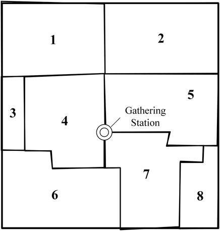
The terrain in the planning area is divided by FCM algorithm. The annual sunshine durations, average altitude, slope direction, slope, the distance between the terrain center and the GS, and the direction of the terrain center relative to the GS in each sub-area are used to complete the terrain clustering. The result is shown in Figure 3.

FIGURE 3

FIGURE 3. The results of terrain division.

After the terrain division, the geographic conditions of each terrain are collected and counted in Table 1. From the Table 1, it can be seen that there are great differences in geographical conditions among the terrains in the planning area. After the terrain is divided, the relationship between meteorological factors and PV output power can be analyzed more accurately, and then more accurate PV expected annual output power can be obtained.

TABLE 1

TABLE 1. The geographic conditions of each terrain.

3.3 Main meteorological factors selection

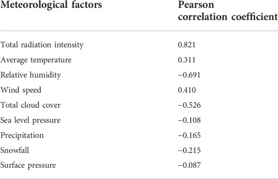
The first step of meteorological analysis is single factor analysis which is aimed to select main meteorological factors. Table 2 presents the results of single meteorological factor analyzed by Pearson correlation. As mentioned in Section 2.2, the Pearson correlation coefficient is a value between −1 and 1. The closer the absolute value of Pearson correlation coefficient is to 1, the stronger the correlation between this meteorological factor and PV output power is. If the value is positive, the meteorological factor is positively related to the PV output power, otherwise, it is negatively related.

TABLE 2

TABLE 2. The Pearson correlation coefficient of each meteorological factor.

Five main meteorological factors are selected depending on the Pearson correlation coefficient. In this case, the total radiation intensity, average temperature, relative humidity, wind speed and total cloud cover are selected as the main meteorological factors. Among them, the total sunshine intensity, average temperature and wind speed are positively correlated with PV output power, and the relative humidity and total cloud cover are negatively correlated with PV output power. Moreover, the total sunshine intensity is the most important factors.

3.4 Photovoltaic output power calculation

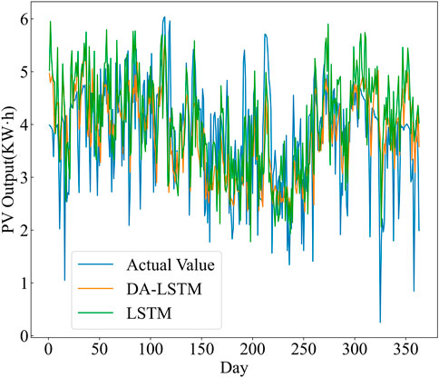
The PV output power and five main meteorological factors data are analyzed by using the DA-LSTM model, and then compared with the ordinary LSTM model. The accuracy of the model is verified by using the root mean square error (RMSE) e_RMSE and the mean absolute error (MAE) e_MAE. In order to analyze the performance of the DA-LSTM model, this paper firstly calculates the output power of the existing PV power plant. This paper compares the calculation results of the DA-LSTM model for PV output power 1 day in advance with the calculation results of the LSTM model without attention mechanism, as shown in Figure 4. It is obvious from Figure 4 that the calculation results of the DA-LSTM model are closer to the real value. Table 3 presents the RMSE and the MAE e_MAE of two different models. The RMSE and MAE produced by DA-LSTM model is smaller than ordinary LSTM, which means the DA-LSTM model performs better in PV output power calculation considering multiple meteorological factors.

FIGURE 4

FIGURE 4. The actual value and the results of different models.

TABLE 3

TABLE 3. The performances of different models.

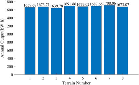
After verifying the accuracy of the DA-LSTM model, the annual expected output power of a single PV panel in each terrain in the planning area is calculated, as shown in Figure 5. It can be seen that there is a certain difference in the output power of PV panels in different terrain. Considering the annual total sunshine intensity and annual sunshine durations of each terrain, it can be found that places with good solar resources are not necessarily the regions with the largest PV output power. That is because other meteorological factors do have a visible impact on PV output. In addition, terrain 7 has the highest PV output power. Moreover, since there are a large number of PV panels in a PV power plant, the priority of the installation site has a great impact on the output power of the final PV power plant.

FIGURE 5

FIGURE 5. The annual expected output power of a single PV panel in each terrain.

3.5 Results of photovoltaic panel deployment

The deployment method proposed in this paper also considers conventional capacity constraints, area constraints and so on. However, its characteristic is that its objective function considers the maximum actual PV output power. To analyze the benefits of the method proposed in this paper, scheme B and C are set as comparison, and the proposed method is scheme A. The difference between the comparison methods is mainly in the objective function, which considers the maximum total sunshine intensity and the maximum total sunshine durations respectively. The PV resource parameters required by the three different methods are shown in Table 4. The parameters required by the two methods for comparison are easy to obtain.

TABLE 4

TABLE 4. The PV resource parameters of each terrain.

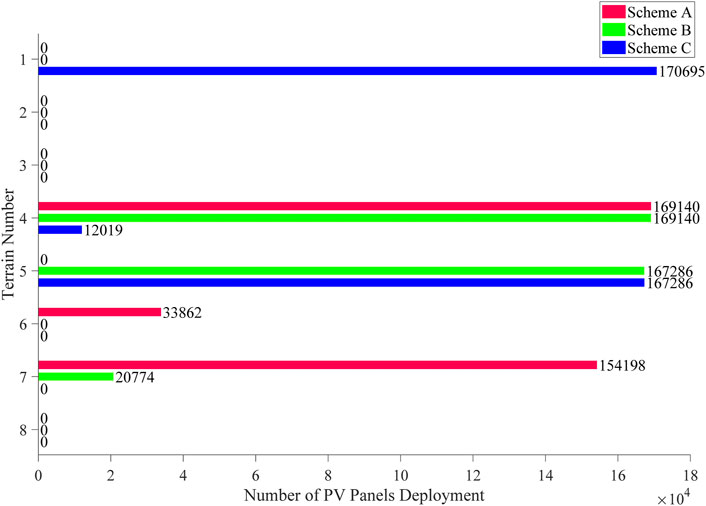
Figure 6 shows the deployment results of three different methods. Obviously, the installation location and quantity of PV panels are different under three methods. Also, it is not difficult to understand that, considering the minimum cost, all deployment method will prefer to select the terrain nearest to the collection station. Terrain 4, 5, 7 are the nearest, therefore, these terrains are given high priority to install PV panels. But the actual deployment of each terrain depends on constraints and different objective functions. It is worth noting that all three methods choose to install a certain number of PV panels on terrain 4, which also proves that terrain four is the best comprehensively.

FIGURE 6

FIGURE 6. The deployment results of three different methods.

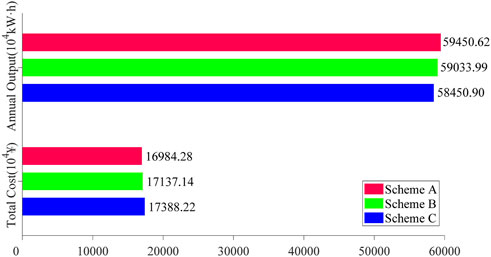
Figure 7 shows the deployment performance of three different methods. Obviously, the installation location and quantity results of three different methods are different. When the estimated PV installed capacity is given, it can be seen that the PV expected output of the purposed method is higher than that of the methods for comparison. The proposed method increases the expected output power by 0.71% and 1.71% compared with scheme B and scheme C respectively. Scheme A also lower the cost, which reduces the cost by 0.89% and 2.32% compared with scheme B and scheme C, respectively. Comparing the effects of the three deployment schemes, we can see that the method proposed in this paper improves the annual PV output power and reduces the total construction cost. In other words, the proposed method effectively improves the efficiency of solar energy utilization and creates higher economic and environmental value.

FIGURE 7

FIGURE 7. The deployment performance of three different methods.

4 Conclusion

An optimization method for the deployment of PV panels in a centralized PV power plant under multiple meteorological and geographical factors is proposed. When deploying PV panels, the geographical and meteorological condition differences in various terrains of the planning area are fully considered, so as to obtain the maximum PV output power. Taking a planning area and an nearby existing PV power plant as examples, the data of interest are collected for case studies and the results of case studies are analyzed.

Considering that the PV panels in the centralized PV power plant are densely arranged during installation, the connectivity between the sub-areas is taken into account when dividing the different terrain in the PV power plant, so that the sub-areas in each terrain are not only similar in geographical characteristics, but also adjacent in geographical locations. The proposed terrain division method meets the needs of the PV power plant planning.

Then, Pearson correlation analysis succeeds in main meteorological selection. Moreover, DA-LSTM model has shown acceptable results in PV output power calculation, and successfully calculates the annual PV output power of various terrains in the planning area.

Finally, the advantages of the optimization method based on terrain division and PV output power calculated by DA-LSTM are proved. Compared with the comparison method, the proposed method has higher output power and less construction cost. The application of this method can improve the efficiency of PV resources utilization and create economic and environmental benefits, which promotes the use of PV technology.

Data availability statement

The original contributions presented in the study are included in the article/Supplementary Material, further inquiries can be directed to the corresponding author.

Author contributions

All authors have made substantial contributions to the conception, design of the work; analysis; and drafting of the paper. All authors read and approved the final manuscript.

Funding

This research is supported by the Science and Technology Project of State Grid Sichuan Economic Research Institute (Grant No. SGSCJY00GHJS2200046).

Conflict of interest

Author ZM was employed by the company State Grid Sichuan Electric Power Company.

The remaining authors declare that the research was conducted in the absence of any commercial or financial relationships that could be construed as a potential conflict of interest.

Publisher’s note

All claims expressed in this article are solely those of the authors and do not necessarily represent those of their affiliated organizations, or those of the publisher, the editors and the reviewers. Any product that may be evaluated in this article, or claim that may be made by its manufacturer, is not guaranteed or endorsed by the publisher.

References

Agoua, X. G., Girard, R., and Kariniotakis, G. (2018). Short-term spatio-temporal forecasting of photovoltaic power production. IEEE Trans. Sustain. Energy 9 (2), 538–546. doi:10.1109/tste.2017.2747765

CrossRef Full Text | Google Scholar

Al-Rousan, N., Isa, N. A. M., and Desa, M. K. M. (2018). Advances in solar photovoltaic tracking systems: A review. Renew. Sustain. Energy Rev. 82, 2548–2569. doi:10.1016/j.rser.2017.09.077

CrossRef Full Text | Google Scholar

Benmouiza, K., Tadj, M., and Cheknane, A. (2016). Classification of hourly solar radiation using fuzzy c-means algorithm for optimal stand-alone PV system sizing. Int. J. Electr. Power & Energy Syst. 82, 233–241. doi:10.1016/j.ijepes.2016.03.019

CrossRef Full Text | Google Scholar

Cheng, L., Zang, H., Ding, T., Wei, Z., and Sun, G. (2021). Multi-meteorological-factor-based graph modeling for photovoltaic power forecasting. IEEE Trans. Sustain. Energy 12 (3), 1593–1603. doi:10.1109/tste.2021.3057521

CrossRef Full Text | Google Scholar

Cotfas, D. T., and Cotfas, P. A. (2019). Multiconcept methods to enhance photovoltaic system efficiency. Int. J. Photoenergy 2019, 1–14. doi:10.1155/2019/1905041

CrossRef Full Text | Google Scholar

Dong, C., Zhou, R., and Li, J. (2021). Rushing for subsidies: The impact of feed-in tariffs on solar photovoltaic capacity development in China. Appl. Energy 281, 116007. doi:10.1016/j.apenergy.2020.116007

CrossRef Full Text | Google Scholar

Ettah, E., Ekah, U., Oyom, E., and Akonjom, N. (2021). Performance analysis of monocrystalline and polycrystalline solar panels in a semi-arid region. Int. J. Eng. Sci. Invent. 10 (7), 10–14. doi:10.35629/6734-1007011014

CrossRef Full Text | Google Scholar

Gowid, S., and Massoud, A. (2020). A robust experimental-based artificial neural network approach for photovoltaic maximum power point identification considering electrical, thermal and meteorological impact. Alexandria Eng. J. 59 (5), 3699–3707. doi:10.1016/j.aej.2020.06.024

CrossRef Full Text | Google Scholar

Greff, K., Srivastava, R. K., Koutnik, J., Steunebrink, B. R., and Schmidhuber, J. (2017). Lstm: A search space odyssey. IEEE Trans. Neural Netw. Learn. Syst. 28 (10), 2222–2232. doi:10.1109/tnnls.2016.2582924

PubMed Abstract | CrossRef Full Text | Google Scholar

Hachicha, A. A., Al-Sawafta, I., and Said, Z. (2019). Impact of dust on the performance of solar photovoltaic (PV) systems under United Arab Emirates weather conditions. Renew. Energy 141, 287–297. doi:10.1016/j.renene.2019.04.004

CrossRef Full Text | Google Scholar

Hashemizadeh, A., Ju, Y., and Dong, P. (2019). A combined geographical information system and Best–Worst Method approach for site selection for photovoltaic power plant projects. Int. J. Environ. Sci. Technol. (Tehran). 17 (4), 2027–2042. doi:10.1007/s13762-019-02598-8

CrossRef Full Text | Google Scholar

Huld, T. (2017). Pvmaps: Software tools and data for the estimation of solar radiation and photovoltaic module performance over large geographical areas. Sol. Energy 142, 171–181. doi:10.1016/j.solener.2016.12.014

CrossRef Full Text | Google Scholar

Ingenhoven, P., Belluardo, G., Makrides, G., Georghiou, G. E., Rodden, P., Frearson, L., et al. (2019). Analysis of photovoltaic performance loss rates of six module types in five geographical locations. IEEE J. Photovolt. 9 (4), 1091–1096. doi:10.1109/jphotov.2019.2913342

CrossRef Full Text | Google Scholar

Jarvis, A., Reuter, H. I., Nelson, A., and Guevara, E. (2008). “Hole-filled SRTM for the globe,” in CGIAR-CSI SRTM 90m database, 4. [Dataset] Available: http://srtm.csi.cgiar.org.

Google Scholar

Kim, G. G., Choi, J. H., Park, S. Y., Bhang, B. G., Nam, W. J., Cha, H. L., et al. (2019). Prediction model for PV performance with correlation analysis of environmental variables. IEEE J. Photovolt. 9 (3), 832–841. doi:10.1109/jphotov.2019.2898521

CrossRef Full Text | Google Scholar

Li, Y., Wang, Y., and Chen, Q. (2020). Study on the impacts of meteorological factors on distributed photovoltaic accommodation considering dynamic line parameters. Appl. Energy 259, 114133. doi:10.1016/j.apenergy.2019.114133

CrossRef Full Text | Google Scholar

Li, J., Chen, S., Wu, Y., Wang, Q., Liu, X., Qi, L., et al. (2021). How to make better use of intermittent and variable energy? A review of wind and photovoltaic power consumption in China. Renew. Sustain. Energy Rev. 137, 110626. doi:10.1016/j.rser.2020.110626

CrossRef Full Text | Google Scholar

Mayer, M. J. (2021). Effects of the meteorological data resolution and aggregation on the optimal design of photovoltaic power plants. Energy Convers. Manag. 241, 114313. doi:10.1016/j.enconman.2021.114313

CrossRef Full Text | Google Scholar

Mekhilef, S., Saidur, R., and Kamalisarvestani, M. (2012). Effect of dust, humidity and air velocity on efficiency of photovoltaic cells. Renew. Sustain. Energy Rev. 16 (5), 2920–2925. doi:10.1016/j.rser.2012.02.012

CrossRef Full Text | Google Scholar

Mensour, O. N., El Ghazzani, B., Hlimi, B., and Ihlal, A. (2019). A geographical information system-based multi-criteria method for the evaluation of solar farms locations: A case study in souss-massa area, southern Morocco. Energy 182, 900–919. doi:10.1016/j.energy.2019.06.063

CrossRef Full Text | Google Scholar

Nayak, J., Naik, B., and Behera, H. S. (2015). “Fuzzy C-means (FCM) clustering algorithm: A decade review from 2000 to 2014,” in Computational intelligence in data mining - volume 2, 133–149.

CrossRef Full Text | Google Scholar

Nogueira, C. E. C., Bedin, J., Niedzialkoski, R. K., de Souza, S. N. M., and das Neves, J. C. M. (2015). Performance of monocrystalline and polycrystalline solar panels in a water pumping system in Brazil. Renew. Sustain. Energy Rev. 51, 1610–1616. doi:10.1016/j.rser.2015.07.082

CrossRef Full Text | Google Scholar

Qu, J., Qian, Z., and Pei, Y. (2021). Day-ahead hourly photovoltaic power forecasting using attention-based CNN-LSTM neural network embedded with multiple relevant and target variables prediction pattern. Energy 232, 120996. doi:10.1016/j.energy.2021.120996

CrossRef Full Text | Google Scholar

Rodríguez, F., Galarza, A., Vasquez, J. C., and Guerrero, J. M. (2022). Using deep learning and meteorological parameters to forecast the photovoltaic generators intra-hour output power interval for smart grid control. Energy 239, 122116. doi:10.1016/j.energy.2021.122116

CrossRef Full Text | Google Scholar

Sengupta, S., Sengupta, S., Chanda, C. K., and Saha, H. (2021). Modeling the effect of relative humidity and precipitation on photovoltaic dust accumulation processes. IEEE J. Photovolt. 11 (4), 1069–1077. doi:10.1109/jphotov.2021.3074071

CrossRef Full Text | Google Scholar

Shewalkar, A., Nyavanandi, D., and Ludwig, S. A. (2019). Performance evaluation of deep neural networks applied to speech recognition RNN, LSTM and GRU. J. Artif. Intell. Soft Comput. Res. 9 (4), 235–245. doi:10.2478/jaiscr-2019-0006

CrossRef Full Text | Google Scholar

Son, N., and Jung, M. (2020). Analysis of meteorological factor multivariate models for medium- and long-term photovoltaic solar power forecasting using long short-term memory. Appl. Sci. 11 (1), 316. doi:10.3390/app11010316

CrossRef Full Text | Google Scholar

Yan, J., Hu, L., Zhen, Z., Wang, F., Qiu, G., Li, Y., et al. (2021). Frequency-domain decomposition and deep learning based solar PV power ultra-short-term forecasting model. IEEE Trans. Ind. Appl. 57 (4), 3282–3295. doi:10.1109/tia.2021.3073652

CrossRef Full Text | Google Scholar

Zeng, Z., Jin, G., Xu, C., Chen, S., Zeng, Z., and Zhang, L. (2022). Satellite telemetry data anomaly detection using causal network and feature-attention-based LSTM. IEEE Trans. Instrum. Meas. 71, 1–21. doi:10.1109/tim.2022.3151930

CrossRef Full Text | Google Scholar

Zhang, H., Wu, K., Qiu, Y., Chan, G., Wang, S., Zhou, D., et al. (2020). Solar photovoltaic interventions have reduced rural poverty in China. Nat. Commun. 11 (1), 1969. doi:10.1038/s41467-020-15826-4

PubMed Abstract | CrossRef Full Text | Google Scholar

Zhang, J., Zhang, B., Li, Q., Zhou, G., Wang, L., Li, B., et al. (2021). Integrated energy production unit: An innovative concept and design for energy transition toward low-carbon development. CSEE J. Power Energy Syst. 7 (6), 1133–1139. doi:10.17775/CSEEJPES.2021.05950

CrossRef Full Text | Google Scholar

Zhu, K., Li, Y., Mao, W., Li, F., and Yan, J. (2022). LSTM enhanced by dual-attention-based encoder-decoder for daily peak load forecasting. Electr. Power Syst. Res. 208, 107860. doi:10.1016/j.epsr.2022.107860

CrossRef Full Text | Google Scholar

Ziane, A., Necaibia, A., Sahouane, N., Dabou, R., Mostefaoui, M., Bouraiou, A., et al. (2021). Photovoltaic output power performance assessment and forecasting: Impact of meteorological variables. Sol. Energy 220, 745–757. doi:10.1016/j.solener.2021.04.004

CrossRef Full Text | Google Scholar