Solar energy digitalization at high latitudes: A model chain combining solar irradiation models, a LiDAR scanner, and high-detail 3D building model

Solar mapping can contribute to exploiting more efficiently the solar energy potential in cities. Solar maps and 3D solar cadasters consist of visualization tools for solar irradiation analysis on urban surfaces (i.e., orography, roofs, and façades). Recent advancements in solar decomposition and transposition modeling and Light Detection and Ranging (LiDAR) scanning enable high levels of detail in 3D solar cadasters, in which the façade domain is considered beside the roof. In this study, a model chain to estimate solar irradiation impinging on surfaces with different orientations at high latitudes is developed and validated against experimental data. The case study is the Zero Emission Building Laboratory in Trondheim (Norway). The main stages of the workflow concern (1) data acquisition, (2) geometry detection, (3) solar radiation modeling, (4) data quality check, and (5) experimental validation. Data are recorded from seven pyranometers installed on the façades (4), roof (2), and pergola (1) and used to validate the Radiance-based numerical model over the period between June 21st and September 21st. This study investigates to which extent high-resolution data sources for both solar radiation and geometry are suitable to estimate global tilted irradiation at high latitudes. In general, the Radiance-based model is found to overestimate solar irradiation. Nonetheless, the hourly solar irradiation modeled for the two pyranometers installed on the roof has been experimentally validated in accordance with ASHRAE Guideline 14. When monthly outcomes are considered for validation, the east and the south pyranometers are validated as well. The achieved results build the ground for the further development of the 3D solar cadaster of Trondheim.

1 Introduction

Solar mapping represents a commonly used visualization technique to support urban planners, authorities, and architects in addressing onsite energy generation while enhancing daylight and sunlight accessibility in buildings (Good et al., 2014; Lobaccaro et al., 2017). The solar potential of urban surfaces (i.e., orography, roofs, and façades) permits providing inputs to the predesign of solar installations in order to develop optimal exploitation of solar energy through generalized planning recommendations, guidelines, and best practices. The efficacy of these models varies considerably due to the following modeling strategy: the accuracy depends on the spatial information available and generated (e.g., satellite data and data from a Light Detection and Ranging (LiDAR) scanner) and the associated level of detail (LoD) of three-dimensional (3D) models (Behar et al., 2015). A popular modeling assumption is that building façades are vertical and that 3D building models can be extruded from 2D roof planes (i.e., 2.5D building models). Current developments in these research fields aim to create more precise information layers to estimate solar system integration not only on roofs (Brito et al., 2012; Desthieux et al., 2018), which are mostly devoid of building infrastructure (e.g., chimneys, elevator lift engines, technical installations, terraces, and balconies) that are common constraints for optimal solar system installation, but also on the non-negligible vertical surfaces (i.e., façades) (Carneiro et al., 2010). In fact, the total surface of the building’s envelope is usually strongly reduced by the shading of architectural elements and obstructions and by the presence of glazed surfaces, which can only be partially replaced with PV systems. In Lobaccaro et al. (2019), a reduction factor, which is related to architectural and geometrical building features, is applied to account for transparent surfaces and obstructions, reducing the solar energy potential of roofs and façades. Although limited to the roof spatial domain, an advanced approach for detecting buildings’ superstructures, which is based on deep learning for the semantic 3D city model, is proposed by Krapf et al. (2022). Estimating solar irradiation on façades including transparent surfaces and obstructions is therefore challenging, and it represents a significant limitation when it comes to high latitude locations where the façades are characterized by a solar potential similar to the roofs in the intermediate seasons (Manni et al., 2018).

In a reliable solar map, an accurate solar radiation model is coupled to a 3D urban geometry with a high LoD. Numerous solar radiation models have been implemented to enable assessing solar energy accessibility at multiple scales, ranging from building components to neighborhoods and cities (Peronato et al., 2018; Boccalatte et al., 2022; De Luca et al., 2022). The solar potential of buildings is analyzed by considering dynamic shadowing, solar inter-building reflections, and other related complex urban phenomena (e.g., high surface temperature and air flow) (Jakica, 2018; Manni et al., 2020). Moreover, high-resolution solar data can be exploited to evaluate instantaneous events, e.g., cloud and albedo enhancement effects (Gueymard, 2017). Advanced solar radiation models allow to identify the most irradiated building surfaces for solar system installations or to evaluate the integration of solar systems in a heritage-constrained environment. Nonetheless, the application of such accurate numerical models to solar mapping at the city scale is still challenging due to the significant computational time.

Several studies have presented procedures to evaluate the solar energy potential in urban areas based on different techniques that have been developed in the last few decades together with the advancement of digital technologies and innovative approaches, methods, and tools. In Brito et al. (2012), the LiDAR technique was coupled to the Solar Analyst tool to estimate the photovoltaic (PV) potential of the Lisbon urban region. Thebault et al. (2022) proposed a multicriteria approach based on a geographic information system (GIS) to evaluate the suitability of a building to be equipped with PV systems. Similarly, a statistical model based on 2D-GIS and multiple linear regression has been developed by Nouvel et al. (2015) to predict heat demand and energy saving potential of building stock at several scales within the city of Rotterdam.

With the development of remote sensing technology and the increase of the available computational capacity, many new methods and technologies were proposed to enable the automatic collection of 3D information about buildings and other target objects (e.g., urban infrastructures and terrain morphology) (Bonczak and Kontokosta, 2019). Geometrical models characterized by a high LoD can be generated through an unmanned aerial vehicle (UAV) and terrestrial laser scanning (TLS) for data collection. The LiDAR technology integrates a laser scanner, the Global Positioning System (GPS), and inertial navigation systems (INS) to produce point clouds for buildings (Zhou and Gong, 2018; Yastikli and Cetin, 2021). The point clouds can provide high-resolution and accurate geometry information for the whole building, including windows, balconies, and other façade architectural elements. Laser scanning can bring 3D point clouds with very high density (with ca. < 1 cm point distance) that are usually post-processed to reduce noise and outliers applying probabilistic approaches such as the one proposed by Min and Meng (2019). The point clouds can significantly contribute to the reconstruction of high-LoD 3D models at multiple scales. Several studies investigate methods to build the 3D model from LiDAR’s outputs, proposing reliable automatic or semi-automatic workflows, even if limited to LoD1 and LoD2 3D models (Sajadian and Arefi, 2014; Yastikli and Cetin, 2017; Jayaraj and Anandakumar, 2018). In fact, automatic reconstruction methods for models with LoD3 or LoD4, including windows and other façade semantic information, are still in the preliminary development phase (Wen et al., 2019; Cao and Scaioni, 2021).

2 Motivation and goals

Within this framework, the present study aims at investigating the application of advanced solar mapping techniques to high latitude locations. The research core concerns both 3D geometry construction workflows and approaches to solar radiation modeling, with a specific focus on input solar datasets. In fact, the study allows one to determine whether satellite-based solar irradiance data and the LiDAR scan technique are suitable to estimate the global tilted irradiation (GTI) for different orientations of solar sensors (i.e., pyranometers) at high latitudes. The results from the numerical model will be validated against measurement data from the Zero Emission Building (ZEB) Laboratory (Nocente et al., 2021) in Trondheim, Norway, presented in section 3.2.

The motivation of this work states the fact that solar maps that have been implemented for low latitudes (e.g., southern Europe and continental Europe) need to be further developed before being efficiently exploited at high latitudes. For instance, the proper spatial domain of solar maps which is usually limited to rooftop surfaces must be extended to façade surfaces as well. In that regard, the sun geometry in the Nordics (i.e., low sun elevation angles) is favorable for such vertical surfaces, which have higher solar potential than roofs (Manni et al., 2018). To model the solar energy potential of building façades in an articulated urban environment, it is necessary to accurately simulate inter-building optical interactions (i.e., mutual reflections and complex shading phenomena) by increasing the LoD of the 3D model and defining the optical properties of the materials applied to urban surfaces.

The novelty of the hereby presented study is grounded around the exploitation of a LoD3 3D model as a geometry base layer for solar irradiation mapping and the validation of the numerical model for multiple orientations at high latitudes. The vertical scanning of the building envelope enables a more precise construction of both the footprint and the façade’s morphology. On the other hand, the extensive monitoring apparatus of solar irradiation that is installed in the ZEB Laboratory permits to perform an experimental validation of the numerical model for the main orientations of the building surfaces. A similar availability of observation data is not present in similar studies carried out for high latitude locations.

The present study is structured as follows: the Introduction (Section 1) outlines a theoretical framework for solar mapping techniques; the Motivation and goals section identifies the reasons for conducting such a study (Section 2); the Methodology section (Section 3) defines the research workflow, the tools for solar analysis and their settings, the information about the case study, the solar data sources, the quality check scheme, the geometry definition process, and the statistical indicators and validation criteria; the Results and Discussion section (Section 4) provides an overview of the capability of the numerical model to simulate the GTI for various orientations, followed by the validation test and the limitations of the study. The article concludes by considering future developments and summarizing the most relevant findings and the implications for future advancements in the implementation of solar maps at high latitudes (Section 5).

3 Methodology

3.1 Workflow

The workflow (Figure 1) proposed and followed in this study is built around five main stages, which are 1) data acquisition, 2) geometry detection, 3) solar radiation modeling, 4) data quality check, and 5) experimental validation (Figure 1). The first stage (stage 1) concerns the acquisition of data about urban geometry, solar irradiation, and weather variables from different online databases, e.g., the Trondheim municipality’s database, solar radiation service from the Copernicus Atmosphere Monitoring Service (CAMS), and climate.onebuilding.org database¹. The user-defined inputs of this stage are the case study’s location and the time interval to investigate. The 3D model of Trondheim contains information about both buildings and terrain. Rhinoceros and Grasshopper tools are used, respectively, to edit the geometry model and select the spatial domain for the solar analysis. A circular area of radius 100 m with the center located in the ZEB Laboratory is selected. Regarding the solar irradiance and weather variables, a Python script is implemented to retrieve such data from the respective databases and combine them into a new EnergyPlus weather file (.epw). In particular, the new .epw file combines solar irradiation values, e.g., direct normal irradiation (DNI), diffuse horizontal irradiation (DHI), and Global Horizontal Irradiation (GHI), from CAMS solar radiation, with the weather variables, e.g., dew point temperature, relative humidity, and cloud cover, from the typical meteorological year (TMY) of Trondheim. The TMY of Trondheim is defined according to the measurements taken at the weather station in Voll (Trondheim) over the 2007–2021 period. The solar irradiation values from CAMS solar radiation are preferred to the values from the TMY since they are based on satellite observations performed during the specific time interval and for the exact location of the case study.

FIGURE 1

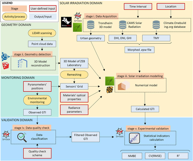
FIGURE 1. Overview of the workflow followed in this study. The main domains (e.g., solar irradiation domain, geometry domain, monitoring domain, and validation domain) are highlighted with different colors, while in the left corner, the four block typologies (e.g., stage, user-defined input, activity/process, and output/input) are reported.

The geometry detection stage (stage 2) moves from the LiDAR scanning campaign of the ZEB Laboratory. Point cloud data are generated as output of the scanning activity, and it is regarded as the reference to detect and reconstruct the geometry of the building and its components (e.g., windows, doors, pergola, and the pattern of building-integrated PV (BIPV) panels). The 3D model is then re-meshed to provide more refined bases for the simulation sensors’ grid. Sensors’ position is also determined according to the location of the pyranometers, whose measurements are used in the experimental validation of the numerical model.

The urban geometry, the 3D model of the ZEB Laboratory, the sensors’ grid, and the morphed .epw file are among the inputs of the numerical model for solar analyses (stage 3). In addition to these, the optical properties of each surface and the Radiance parameters (e.g., ambient accuracy (aa), ambient bounces (ab), ambient division (ad), and ambient resolution (ar)) must be defined. The output from the solar irradiation modeling consists of a time series of simulated GTI values for each sensor (i.e., pyranometer).

In stage 4, the solar irradiation data from measurements in the ZEB Laboratory are classified according to the quality check scheme described in section 3.5. A quality flag is associated with each datapoint and then used to filter the observed GTI quantities to exclude the erroneous measurements from the validation process.

Finally, the simulated GTI was validated against observations (stage 5). The two datasets are visually compared in scatter plots; one graph is created for each pyranometer. Moreover, three statistical indicators, namely, the normalized mean bias error (NMBE), the coefficient of variation of the root mean square error CV(RMSE), and the coefficient of determination (R²), are calculated to evaluate the model’s accuracy.

3.2 Case study

The ZEB Laboratory² is used as a case study for this research. Located in Trondheim, Norway (63.41 N, 10.4 E), the ZEB Laboratory is a four-story high office building (Nocente et al., 2021), designed and realized as a pilot building to facilitate the diffusion of innovative components, solutions, and energy strategies in the building industry. The load-bearing structure consists of glued laminated timber (gluelam) columns, cross-laminated timber (CLT) floors, some stiffening inner walls, and traditional insulated wooden framework in the outer walls. The whole building is constructed according to the ZEB-COM ambition (Lobaccaro et al., 2018), which means that the local production of renewable energy must compensate, in terms of equivalent CO₂, the materials, the construction process, and the operation for 60 years, which is the programmed life of the building. To achieve this ambition, most of the building envelope is covered in BIPV, PV being the main source of renewable energy. A total of 701 mono-Si BIPV panels are installed for a rated power of 184 kW_p. According to simulations, the system can deliver over 150 MWh/y of renewable energy, partly used on the spot, while the rest is delivered to the grid.

The presence of such an extensive installation, together with the advanced monitoring and control system, allows the building to produce a high quantity of data, making the ZEB Laboratory a valuable source for studying BIPV operation in a Nordic climate and over a long period of time (i.e., the life of the PV installation). To have a reference for the outdoor weather and the available solar radiation, the laboratory is equipped with many outdoor sensors. A weather station is installed on the roof, continuously registering the main meteorological parameters. Another weather station is installed on the ground toward the south. The measurement of the available solar resources is performed by second-class pyranometers. One pyranometer registers the radiation on the horizontal plane, while five others evaluate the radiation on the planes of each façade and the roof. As shown in Figure 2, a pergola is mounted outside of the building, and it is entirely constituted by PV panels in a chessboard distribution of opaque and semi-transparent modules. Both surfaces of the pergola, the external and the internal ones, are equipped with pyranometers. The panels of the whole building (i.e., BIPV and the pergola’s PV) are connected in strings, and the solar power production can be monitored and registered at any time.

FIGURE 2

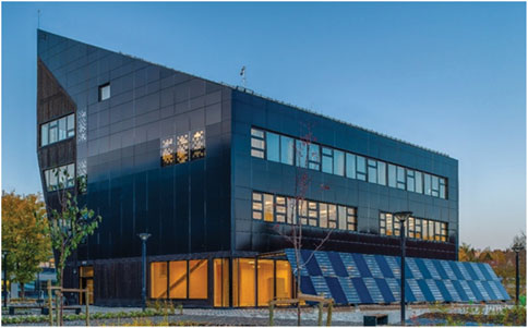
FIGURE 2. ZEB Laboratory: southern and western façade (^© Photo: M. Herzog).

3.3 Tools and settings

Solar analyses are performed within the Grasshopper environment. The Honeybee (HB) environmental plugin is exploited to connect Grasshopper to the Radiance-based engine, coupling the features of such a daylighting and solar simulation tool to the parametric modeling principles implemented in Grasshopper. The “HB annual irradiance” component enables computing broadband solar irradiance considering multiple and mutual inter-building reflections. Input parameters are the weather data, the geometry and optical properties of the model’s surfaces, the grid of sensors, and the Radiance parameters. The weather data are retrieved for the Trondheim location (see section 3.4 for the weather input data).

When it comes to geometry modeling, the 3D model of the ZEB Laboratory is implemented starting from the data provided by the LiDAR scanner. The geometry configuration of the surrounding area is provided by the 3D model from the municipality of Trondheim³. All the materials applied to the urban surfaces are considered opaque and clustered into four groups; each group is characterized by a unique combination of reflection and specularity coefficients. A reflection coefficient of 0.10 and a specularity coefficient of 0.6 are associated with the BIPV and installed on the pergola (see section 3.2) and the glazed surfaces. The charred timber coating covering the other part of the building’s façade is defined as completely diffusive, with a reflection coefficient of 0.25. The same reflection coefficient is defined for the building surrounding the ZEB Laboratory. Finally, the ground is fully diffusive, and it is characterized by a reflection coefficient of 0.10.

The grid of sensors is applied to the geometry moving from the triangular and quadrangular meshes composing the 3D model of the ZEB Laboratory. The centers and the normal vectors of the meshes are considered inputs for the locations and directions (i.e., orientations) of the sensors. The density of the resulting virtual sensors’ point cloud is averagely equal to two points per square meter, but higher density values are observed in complex building areas (i.e., windows and frames). Once the solar analysis is performed, only the points of the grid that are near to the location of the pyranometers are considered for the validation.

Radiance parameters are determined according to the best practices identified in the literature to achieve a high quality of outcomes. An overview of the selected Radiance parameters is reported in Table 1.

TABLE 1

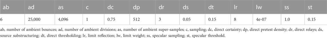
TABLE 1. Radiance parameters defined in this study.

The outputs are average and peak global irradiation and the cumulative radiation in the year. These data are processed with the “HB annual results to data” and “LB deconstruct data” components to extract hourly amounts of global irradiance, which will be later validated against experimental data.

3.4 Solar data sources

Weather datasets used in this work refer to Trondheim, Norway (lat. 63°25′49.76″N). The climate of Trondheim is classified as continental subarctic climate (Dfc) in the Köppen Geiger classification (Figure 3), and it is moderately continental, with cold winters and mild summers (Beck et al., 2018). The analyses are carried out for the period between June 21st and September 21st. The datasets are characterized by a time resolution of 1 hour. This period of the year was selected to validate the model’s outputs in summer conditions, during days characterized by clear or overcast sky conditions.

FIGURE 3

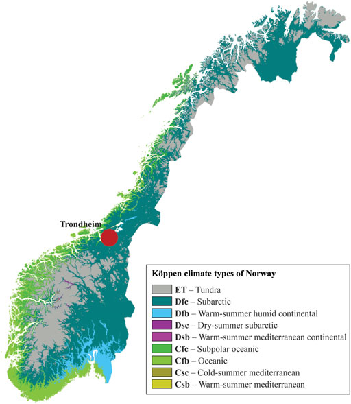
FIGURE 3. Köppen climate classification. Modified from “Köppen climate types of Norway” by Adam Peterson.

The EnergyPlus weather file of Trondheim, created considering monitored values over the years between 2007 and 2021, was retrieved from the repository of free climate data for building performance simulation (<u>climate.onebuilding.org)</u>. Then, the irradiation parameters (GHI, DNI, and DHI) are replaced with values retrieved from the CAMS. The CAMS solar radiation service combines output from the CAMS global forecast system on aerosol and ozone with detailed cloud information directly from geostationary satellites. The CAMS solar radiation service provides, among others, historical values (from 2004 to present) of GHI, DHI, and DNI (both overcast and clear sky conditions) with a time resolution of 1 min. Such irradiance parameters are retrieved for the time interval investigated in this study and resampled hourly.

The GTI is measured by sensors that are either integrated in the building envelope of the ZEB Laboratory or installed on a mast on the roof at a short distance from the surfaces and with accurately measured angles. Installed sensors are second-class pyranometers. The orientation is described in Figure 4 and Table 2. The tilt is reported in degrees from the horizontal surface. Quantities of GTI are recorded with 1-min time resolution and then resampled to calculate average hourly values.

FIGURE 4

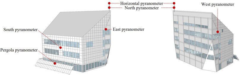
FIGURE 4. Location of the pyranometer in the ZEB Laboratory.

TABLE 2

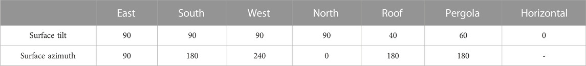
TABLE 2. Orientation of the pyranometers installed in the ZEB Laboratory.

3.5 Quality check scheme for monitored data

The outcomes from the numerical analyses are experimentally validated against quantities measured in the ZEB Laboratory. In order to ensure a good data quality, the quality control scheme described in Lorenz et al. (2022) is applied. Lorenz et al. (2022) implemented a quality control scheme for sensors with different orientations. Their measurement stations consist of a pyranometer for measuring GHI and three silicon cells oriented east, south, and west with tilt angles of 25 for measuring GTI. Such a configuration is similar to the sensors’ layout in the ZEB Laboratory, except that there are pyranometers instead of silicon cells and different orientations are considered (see Table 2). Therefore, only the quality checks for irradiation measurements are considered. Temperature monitoring can in fact be neglected when using pyranometers instead of silicon cells.

Different quality tests are performed for each variable in order to associate a quality flag (QF) to each measure. QFs are later used to filter erroneous measurements. The executed tests consist of the comparison to range limits and the evaluation of sensor consistency. The thresholds identified by Lorenz et al. (2022) are specifically adjusted for our location and sensors, that is, high latitude location and vertically mounted sensors.

A single QF is associated with each value measured; a high number corresponds to a low quality. QFs range between 0 (the test is passed) and 3 (the measurement is most likely erroneous). A value of 1 (QF = 1) indicates that the test cannot be performed, while a value of 2 (QF = 2) stands for a measurement that is likely to be erroneous. The range and consistency limits for all measurement variables are reported in Table 3.

TABLE 3

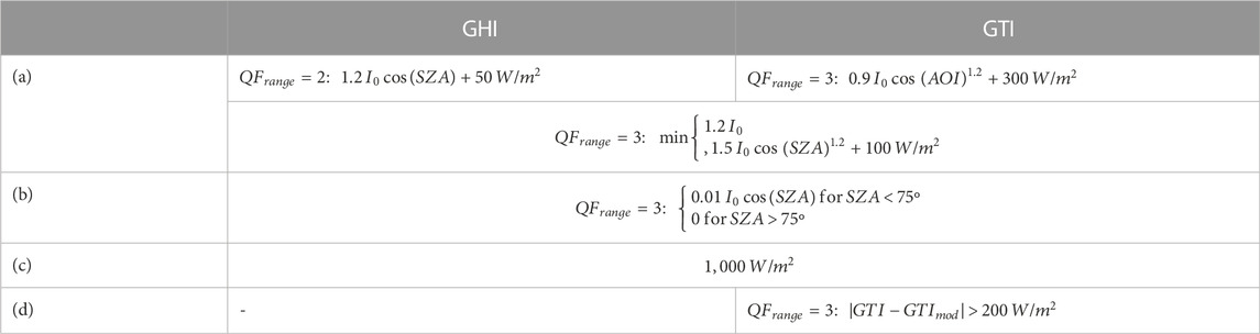
TABLE 3. Upper a) and lower limits b), acceptable max step amount c), and consistency check d) for the measurement of GHI and GTI (Lorenz et al., 2022).

For GHI upper limits, the upper envelope function proposed by Espinar et al. (2011) is applied to determine rare (QF = 2) and extreme (QF = 3) values. The function to define QF = 3 for GTI in the range limit test is adapted from the one proposed for GHI by using angle of incidence instead of solar zenith angle as an input parameter. In regards to consistency check, the GTI is compared to the modeled GTI (GTI_mod): monitored hourly values that differ from the modeled quantity by more than 200 W/m² are classified as QF = 3. The modeled GTI for each pyranometer is calculated from the measured GHI which is considered as input in the model chain described in the following lines. The Engerer2 model (Bright and Engerer, 2019) is applied to decompose the measured GHI into direct and diffuse fractions, and then, the Perez model (Perez et al., 1990) is exploited to transpose them according to the surface azimuth and tilt angle. The model chain applied in the consistency test differs from the one that is validated in this study (e.g., based on HB), although the output parameters are the same. Consistency quality flags for GHI values are determined by the QFs of GTI data. A detailed description of how the range and the consistency limits are determined can be found in Lorenz et al. (2022).

3.6 Geometry detection

Existing fully automatic methods for geometry detection cannot fit the requirements in terms of LoD that are necessary for the 3D model to be implemented in this study, e.g., the depth of windows, the layout of solar panels, material patterns, architecture element detection/recognition, and reconstruction. Hence, the high-LoD 3D model of the ZEB Laboratory is detected and reconstructed based on point cloud data, with the support of a vertical survey of façades conducted with LiDAR laser scanning techniques. The reconstruction of the high-LoD 3D building model and the further geometry detection need the support of accurate geometry information. To obtain the related geometry and geographic information, the high-density 3D scan data were collected by the Trimble SX10 3D scanning device on June 17, 2022. A total of six scan stations are set up to position the scanning device (Figure 5).

FIGURE 5

FIGURE 5. From the top: (A) scanning operations, (B) view of the point cloud during the scanning operations, and (C) positions of scanning stations around the ZEB Laboratory.

The set point spacing is 2–3 mm, while the average distance between the station points and the building is around 15 m. The multi-station scan data are registered by using Trimble Business Center (TBC) software to generate the 3D point cloud information describing the geometry configuration of the ZEB Laboratory. Following this, the point cloud data are converted into the high-LoD 3D model of the building case study in the SketchUp environment. At the same time, the geometry information for façade elements, e.g., windows, doors, and photovoltaic panels, is also identified.

3.7 Measuring uncertainty and validation criteria

The American Society of Heating, Refrigerating and Air-Conditioning Engineers (ASHRAE) Guideline 14 is (ASHRAE, 2002) considered here as the reference source in the determination of the uncertainty associated with the numerical model (Ruiz and Bandera, 2017). The recommended uncertainty indices are the NMBE, the CV(RMSE), and R².

The NMBE is expressed as a percentage and consists of a normalization of the mean bias error (MBE) index, which is, in turn, the average of the errors in a sample space. Normalizing the MBE enables comparing different outcomes. The general formula to calculate the NMBE is (Eq. 1).

$NMBE=\frac{1}{\overline{o}}\frac{{\sum }_{i=1}^n\left(o_i-s_i\right)}{n-1}·100\%,(1)$

where $\overline{o}$ is the mean of the observed values, $o_i$ is the ith observed value, $s_i$ is the ith simulated value, and n is the number of measured data points. Positive values mean that the numerical model tends to under-predict the measured parameter. On the contrary, negative values indicate an overestimation of the measured parameter. However, the NMBE is also subject to cancellation errors; consequently, the use of this index alone is not recommended.

The CV(RMSE) measures the variability of the errors between observed and simulated values, and it is determined according to (Eq. 2).

$CV\left(RMSE\right)=\frac{1}{\overline{o}}\sqrt{\frac{{\sum }_{i=1}^n{\left(o_i-s_i\right)}^2}{n-1}}·100\%(2)$

It is not subject to cancellation errors; thus, the ASHRAE Guidelines couple it with the NMBE index to verify the models’ accuracy.

The R² index provides information on how close the simulated values are to the regression line of the observed values. It ranges from 0 to 1, where the former indicates a complete mismatch between observed and simulated values and the latter means a perfect match between them. It is calculated as follows:

$R^2={\left(\frac{n{\sum }_{i=1}^n{o}_i{s}_i-{\sum }_{i=1}^n{o}_i{\sum }_{i=1}^n{s}_i}{\sqrt{\left(n{\sum }_{i=1}^n{o}_i^2-{\left({\sum }_{i=1}^n{o}_i\right)}^2\right)}\left(n{\sum }_{i=1}^n{s}_i^2-{\left({\sum }_{i=1}^n{s}_i\right)}^2\right)}\right)}^2.(3)$

When it comes to the calibration of the numerical model, the criteria provided by the ASHRAE Guideline 14 are adopted (Table 4). The document presents different thresholds depending on the time resolution of the outcomes, ranging from hourly to monthly quantities. On the one hand, the NMBE index should be within the interval from -5% to 5% for monthly outcomes and within the interval from -10% to 10% for hourly outcomes. On the other hand, an upper limit of 15 is associated with the CV(RMSE) when monthly analyses are performed. This upper limit is doubled (up to 30) if hourly analyses are carried out. Finally, although the R² is not a prescriptive value for calibrated models, the ASHRAE Handbook recommends that the value be higher than 0.75 for calibrated models.

TABLE 4

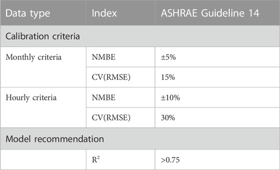
TABLE 4. Validation criteria provided by the ASHRAE Guideline 14.

4 Results and discussion

4.1 Geometry detection

The output point cloud data of the ZEB Laboratory and the corresponding high-LoD 3D model are shown in Figure 6 and Figure 7. Data points collected by the scanner during the campaign are later post-processed by filtering noise and elements from the background and surrounding environment. In total, around 18,600,000 data points are used to build the 3D model.

FIGURE 6

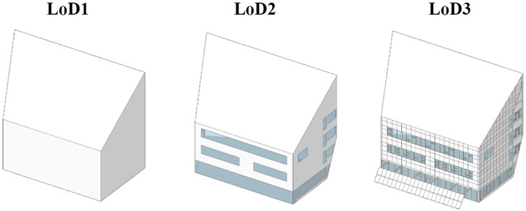
FIGURE 6. Different levels of detail associated with the 3D model of the ZEB Laboratory. The LoD3 is the one achieved in this study.

FIGURE 7

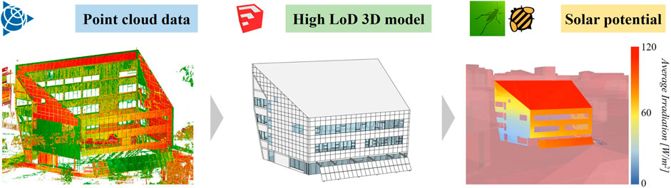
FIGURE 7. Changes in the geometry model from the point cloud data to the high-LoD 3D model of the ZEB Laboratory and to the solar potential analysis.

In general, the LoD3 is preferred to the lower levels (e.g., LoD1 and LoD2) because it allows including all architectural features on the façades (e.g., balconies, frames, doors, windows, and other façade details). In the case of the ZEB Laboratory, the PV pergola and other façades’ elements (e.g., windows and frames) are modeled in high detail. Such elements influence the solar irradiation collected by the south pyranometer and the pyranometer installed on the pergola. In addition to this, the implementation of a LoD3 model in the ZEB Laboratory lays the groundwork for advanced solar energy analyses, where the details of architectural elements are relevant to have more accurate results and for the development of high-LoD solar cadaster. The latter can be coupled to other numerical models to perform energy analyses, visual and thermal comfort assessments, and PV energy simulations.

4.2 Solar analysis

The outcomes from solar analyses performed through the HB plugin and Radiance simulation engine are reported in this section. The solar irradiation impinging on the seven sensors extracted from the grid and representative of the seven pyranometers installed in the ZEB Laboratory is reported in Table 5 and Figure 8.

TABLE 5

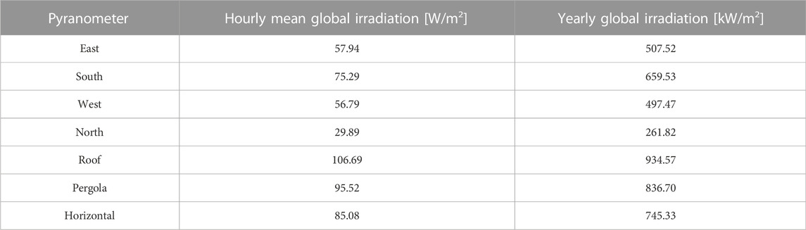
TABLE 5. Hourly mean ad yearly global irradiation over the year for each pyranometer.

FIGURE 8

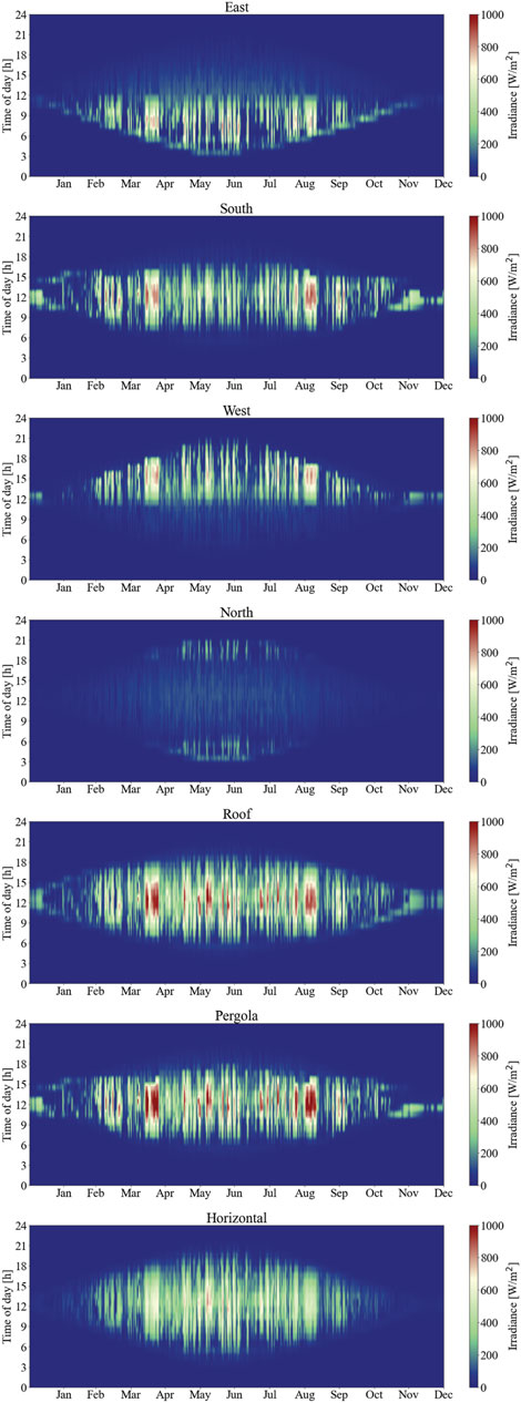
FIGURE 8. Hourly distribution of solar irradiation over the year for each pyranometer.

The three pyranometers facing south with different tilt angles together with the horizontal pyranometer are the most irradiated throughout the year. The pyranometers integrated in the roof, the pergola, and the south façade collect up to 934.57 kWh/m² per year, 836.70 kWh/m² per year, and 659.53 kWh/m² per year, respectively. The solar irradiation impinging on the one horizontally mounted achieves 745.33 kWh/m² per year. Conversely, the pyranometer facing the north is the least irradiated (261.82 kWh/m² per year). Although the west façade is partially shaded by the nearby building, it is still reached and receives almost the same amount of irradiance as the east façade, which is mostly unobstructed (around 500 kWh/m² per year). This is mostly due to the fact that the west façade is not perfectly facing west, that is, the azimuth angle is 240. The irradiation patterns of the west and east façades (Figure 8) highlight this aspect.

4.3 Data quality check

The quality check of the solar irradiation data recorded by the pyranometers integrated in the ZEB Laboratory between June 21st and September 21st is performed by assigning a quality flag to each observation. An overview of these quality flags is presented in Figure 9. The visual inspection of the diagrams suggests that a low level of reliability (QF = 3) is mostly associated either with low solar irradiation amounts or with those values that have been measured during particularly overcast sky conditions.

FIGURE 9

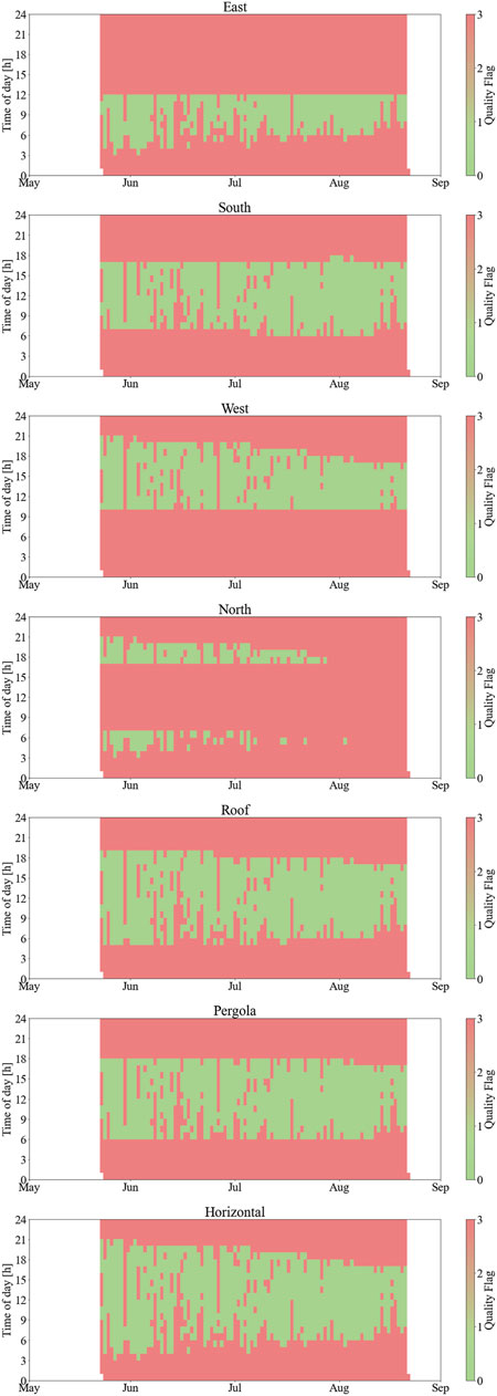
FIGURE 9. Overview of the quality flags associated with the datapoints.

Following this, the datapoints that are suitable to be used in the validation process (QF = 0) are filtered out for each pyranometer. The applied quality check scheme allowed excluding more than 10,000 data points including, among the others, values measured during the night. The resulting datasets differ for the number of values; the dataset affected the most by this reduction is the one from the north-facing pyranometer, which is reduced to around one-tenth (from 2,208 to 212 data points). Among the others, the horizontally mounted pyranometer is the sensor collecting the most reliable data since it shows the highest amount of data with QF = 0 (1,018 data points). This is probably due to the fact that the sensor is exposed to direct sunlight for most of the time during the investigated period, and solar irradiation is usually measured with high accuracy by the pyranometer in this condition. A complete overview of the filtered data for each pyranometer is provided in Figure 9.

4.4 Experimental validation

The solar irradiation outcomes from the numerical model are reported against the experimental observations in the scatter plots in Figure 10. It is worth highlighting that only the values satisfying the requirements of the quality check scheme are included in these graphs. Hence, the length of the datasets changes depending on the considered pyranometer (Table 6).

FIGURE 10

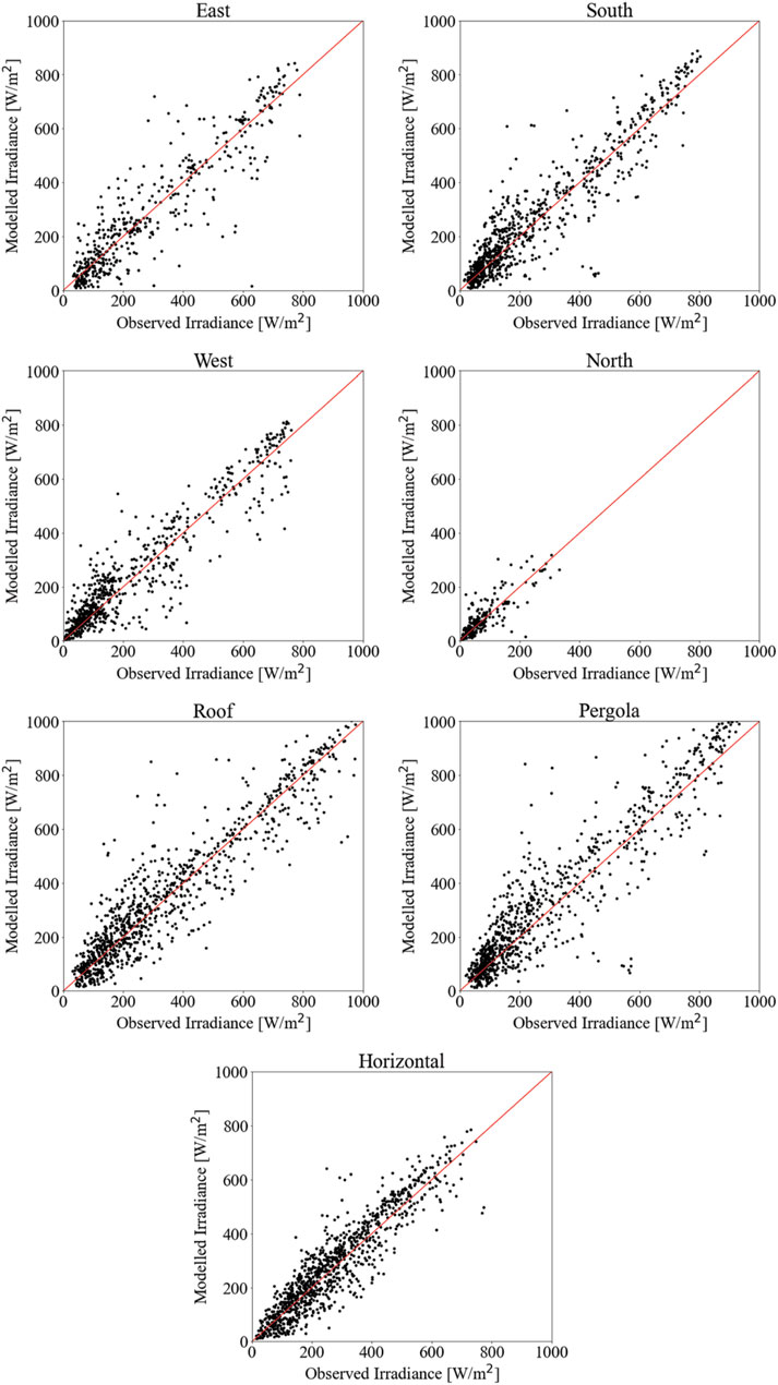
FIGURE 10. Scatter plots with solar irradiation outcomes from the numerical model against the experimental observations.

TABLE 6

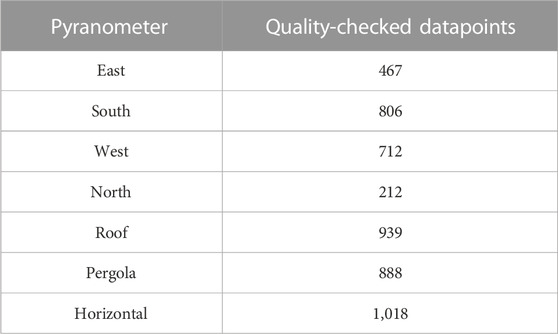
TABLE 6. Datapoints after the application of the quality check scheme.

The visual comparison of the observed and calculated values shows that the numerical model can calculate in a more accurate way the solar irradiation impinging on the horizontal pyranometer and on the roof surface compared to the others. However, the general tendency of the numerical model to overestimate the solar irradiation amounts is clear, as shown by the significant presence of data points above the red line.

The experimental validation is performed according to the ASHRAE Guideline 14 (section 3.7). The statistical indicators and their respective thresholds are considered on both an hourly and monthly basis. When it comes to the hourly solar irradiation amounts, the statistical indicators, e.g., NMBE, CV(RMSE), and R², are estimated for the seven pyranometers (Table 7). The NMBE values are always lower than the threshold identified by the ASHRAE Guideline 14 (i.e., NMBE < ±10%). The negative NMBE values indicate that the numerical model tends to overestimate the solar irradiation quantities, confirming the deductions from the graphs’ observations. The R² amounts always fit ASHRAE’s requirements (i.e., R² > 0.75). However, it is just a recommendation and not a calibration criterion. On the contrary, only the CV(RMSE) values calculated for the roof and horizontal pyranometers are acceptable (i.e., CV(RMSE) < ±30%); therefore, these are the only hourly outcomes from the numerical model that can be validated.

TABLE 7

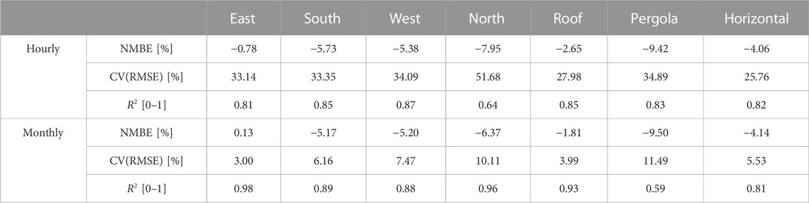
TABLE 7. Statistical indicators estimated for the observed and calculated hourly solar irradiation amounts for each pyranometer.

The east, south, west, and pergola sensors showed CV(RMSE) values that are slightly above the upper limit (30%). In this regard, the exploitation of ground measurements of DNI and DHI as model input in place of the solar radiation data from satellite observation can enhance the result’s accuracy. Finally, the sensor installed in the north façade is the one characterized by the lowest level of accuracy probably because it is the sensor that receives the least radiation, and the main irradiation contribution is usually from the diffuse fraction.

When the statistical indicators are calculated for data aggregated on a monthly basis, the simulated amounts for the east- and south-oriented pyranometers, in addition to the roof and horizontal pyranometers, are labeled as validated (Table 7). In fact, both the NMBE and the CV(RMSE) indicators of these two sensors are within the thresholds from the ASHRAE Guideline 14 (i.e., NMBE < ±5% and CV(RMSE) < ±15%).

In this case, the sensor that is farthest to be validated is the one installed on the pergola. In fact, the pergola is located near the ground; therefore, it is the one mostly affected by human activities happening around the buildings, e.g., the presence of vehicles, and by the optical properties of the ground, e.g., changes in ground reflectivity due to weather conditions.

4.5 Limitations of the study

The main limitations of this study are presented and discussed in the following section. First, data on solar radiation from satellite observations may contain an incorrect estimation of direct and diffuse fractions and systematic errors within the evaluation of the GTI. Ground measurements of solar radiation are more reliable and can overcome this issue. However, satellite observations are available for every location within the spatial domain of CAMS solar radiation, providing up-to-date information. This aspect, together with the possibility of retrieving direct and diffuse solar irradiation data that are not calculated by decomposition models, makes CAMS solar radiation one of the most used and most accepted sources of solar radiation data inputs in solar mapping.

Concerning the 3D model, the optical properties of the materials applied to the urban surfaces are not experimentally determined but retrieved from the literature. This might lead to an incorrect assessment of mutual reflections between the building case study and either the surrounding buildings or the ground surface. Nonetheless, none of the sensors except the ones installed on the pergola and the one facing east have nearby surfaces that can reflect solar radiation toward them, that is, these sensors are installed far from the ground and other buildings.

Finally, the experimental validation is carried out only in summer conditions and for a limited time interval (i.e., 3 months). However, this is the period of the year when the solar irradiation is maximum at high latitudes; hence, it is the one determining the most the solar energy potential of a building. However, further validation studies are planned to be performed to validate the numerical model during intermediate seasons (i.e., spring and fall) when the solar energy potential of façades is significant at high latitudes.

5 Conclusion and future outlooks

A workflow integrating the geometry definition of high-LoD 3D models and the mapping of the solar irradiation is proposed for application at high latitudes. The 3D model of the building case study is reconstructed with the help of laser scanning techniques. The outcomes from the solar radiation model are experimentally validated against data collected from seven pyranometers installed in the ZEB Laboratory in Trondheim. A quality check scheme is applied to reduce the influence of potentially erroneous observations on the statistical indicators.

The findings of this study can be summarized in the following points:

1) The applied quality check scheme allowed excluding more than 10,000 data points that would have decreased the reliability of the experimental validation process.

2) The Radiance-based numerical model tends to overestimate the solar irradiation quantities for all the sensors compared to real measured data recorded with pyranometers.

3) The hourly solar irradiation outcomes of the roof and the horizontal pyranometers are experimentally validated in accordance with the ASHRAE Guideline 14.

4) The monthly solar irradiation outcomes of the east, the south, the roof, and the horizontal pyranometers are validated in accordance with the ASHRAE Guideline 14.

Such results represent a first and significant step toward the implementation of a solar cadaster in Trondheim that will help to enhance the predesign of solar systems and estimation of their solar potential and the social acceptability of solar energy and promote the involvement of stakeholders through the visualization of energy production data and accurate performance predictions. The solar irradiation collected by the façades, which is neglected in the existing 2D solar maps, is experimentally validated against data collected by vertically mounted pyranometers with multiple orientations. Including building façade in solar cadaster is challenging since it requires to accurately model inter-building effects (e.g., mutual shading and reflections). Also, high-detail 3D models like the one implemented in this study are necessary to trace the path covered by sunrays within the investigated spatial domain.

The future developments of this work will be focused on

1) Performing the experimental validation of the numerical model over a longer period, e.g., 1 year.

2) Experimentally validate the south, east, west, and north sensors and the one installed on the pergola by considering ground measurements of direct and diffuse irradiation and integrating decomposition and transposition modeling into the workflow.

3) Enhance the numerical model to perform 1-min solar analyses that enable simulating instantaneous phenomena, e.g., cloud enhancement events.

4) Implement the algorithm to fully automatically detect building geometry and materials applied to surfaces.

Data availability statement

Publicly available datasets were analyzed in this study. This data can be found here: ads.atmosphere.copernicus.eu (CAMS solar radiation service), climate.onebuilding.org (Climate.OneBuilding.Org).

Ethics statement

Written informed consent was obtained from the individual(s) for the publication of any potentially identifiable images or data included in this article.

Author contributions

All authors listed have made a substantial, direct, and intellectual contribution to the work and approved it for publication.

Funding

This research was supported by the Research Council of Norway through the research projects “Enhancing Optimal Exploitation of Solar Energy in Nordic Cities through the Digitalization of the Built Environment” (Helios, project no. 324243) and from NTNU Digital project (project no. 81771593).

Conflict of interest

The authors declare that the research was conducted in the absence of any commercial or financial relationships that could be construed as a potential conflict of interest.

Publisher’s note

All claims expressed in this article are solely those of the authors and do not necessarily represent those of their affiliated organizations, or those of the publisher, the editors, and the reviewers. Any product that may be evaluated in this article, or claim that may be made by its manufacturer, is not guaranteed or endorsed by the publisher.

Footnotes

¹climate.onebuilding.org

²www.zeblab.no

³www.trondheim.kommune.no

References

Ashrae, (2002). Measurement of energy and demand savings. Atlanta, Georgia: American Society of Heating, Ventilating and Air Conditioning Engineers.

Google Scholar

Beck, H. E., Zimmermann, N. E., McVicar, T. R., Vergopolan, N., Berg, A., and Wood, E. F. (2018). Present and future Köppen-Geiger climate classification maps at 1-km resolution. Sci. Data 5, 180214. doi:10.1038/sdata.2018.214

PubMed Abstract | CrossRef Full Text | Google Scholar

Behar, O., Khellaf, A., and Mohammedi, K. (2015). Comparison of solar radiation models and their validation under Algerian climate – the case of direct irradiance. Energy Convers. Manag. 98, 236–251. doi:10.1016/J.ENCONMAN.2015.03.067

CrossRef Full Text | Google Scholar

Boccalatte, A., Thebault, M., Ménézo, C., Ramousse, J., and Fossa, M. (2022). Evaluating the impact of urban morphology on rooftop solar radiation: A new city-scale approach based on geneva GIS data. Energy Build. 260, 111919. doi:10.1016/j.enbuild.2022.111919

CrossRef Full Text | Google Scholar

Bonczak, B., and Kontokosta, C. E. (2019). Large-scale parameterization of 3D building morphology in complex urban landscapes using aerial LiDAR and city administrative data. Comput. Environ. Urban Syst. 73, 126–142. doi:10.1016/J.COMPENVURBSYS.2018.09.004

CrossRef Full Text | Google Scholar

Bright, J. M., and Engerer, N. A. (2019). Engerer2: Global re-parameterisation, update, and validation of an irradiance separation model at different temporal resolutions. J. Renew. Sustain. Energy 11, 033701. doi:10.1063/1.5097014

CrossRef Full Text | Google Scholar

Brito, M. C., Gomes, N., Santos, T., and Tenedório, J. A. (2012). Photovoltaic potential in a Lisbon suburb using LiDAR data. Sol. Energy 86, 283–288. doi:10.1016/j.solener.2011.09.031

CrossRef Full Text | Google Scholar

Cao, Y., and Scaioni, M. (2021). 3DLEB-Net: Label-Efficient deep learning-based semantic segmentation of building point clouds at LoD3 level. Appl. Sci. 11, 8996. doi:10.3390/app11198996

CrossRef Full Text | Google Scholar

Carneiro, C., Morello, E., Desthieux, G., and Golay, F. (2010). VIS ’10. World Scientific and Engineering Academy and Society (WSEAS), Stevens Point, 141–148.Urban environment quality indicators: Application to solar radiation and morphological analysis on built area, Proceedings of the 3rd WSEAS International Conference on Visualization, Imaging and Simulation, Wisconsin, USA.

Google Scholar

De Luca, F., Sepúlveda, A., and Varjas, T. (2022). Multi-performance optimization of static shading devices for glare, daylight, view and energy consideration. Build. Environ. 217, 109110. doi:10.1016/j.buildenv.2022.109110

CrossRef Full Text | Google Scholar

Desthieux, G., Carneiro, C., Camponovo, R., Ineichen, P., Morello, E., Boulmier, A., Abdennadher, N., Dervey, S., and Ellert, C. (2018). Solar energy potential assessment on rooftops and facades in large built environments based on LiDAR data, image processing, and cloud computing. Methodological background, application, and validation in geneva (solar cadaster). Front. Built Environ. 4. doi:10.3389/fbuil.2018.00014

CrossRef Full Text | Google Scholar

Espinar, B., Wald, L., Blanc, P., Hoyer-Klick, C., Schroedter Homscheidt, M., and Wanderer, T. (2011). Project ENDORSE - excerpt of the report on the harmonization and qualification of meteorological data:Procedures for quality check of meteorological data. Paris, France, Europe: Mines ParisTech.

Google Scholar

Good, C. S., Lobaccaro, G., and Hårklau, S. (2014)., 58. Elsevier, 166–171. doi:10.1016/j.egypro.2014.10.424Optimization of solar energy potential for buildings in urban areas - a Norwegian case studyEnergy Procedia

CrossRef Full Text | Google Scholar

Gueymard, C. A. (2017). Cloud and albedo enhancement impacts on solar irradiance using high-frequency measurements from thermopile and photodiode radiometers. Part 2: Performance of separation and transposition models for global tilted irradiance. Sol. Energy 153, 766–779. doi:10.1016/J.SOLENER.2017.04.068

CrossRef Full Text | Google Scholar

Jakica, N. (2018). State-of-the-art review of solar design tools and methods for assessing daylighting and solar potential for building-integrated photovoltaics. Renew. Sustain. Energy Rev. 81, 1296–1328. doi:10.1016/j.rser.2017.05.080

CrossRef Full Text | Google Scholar

Jayaraj, P., and Anandakumar, R. (2018). 3D citygml building modelling from LIDAR point cloud data. Int. Arch. Photogramm. Remote Sens. Spat. Inf. Sci. 5, 175–180. doi:10.5194/isprs-archives-XLII-5-175-2018

CrossRef Full Text | Google Scholar

Krapf, S., Willenborg, B., Knoll, K., Bruhse, M., and Kolbe, T. H. (2022). Deep learning for semantic 3D city model extension: Modeling roof superstructures using aerial images for solar potential analysis. ISPRS Ann. Photogramm. Remote Sens. Spat. Inf. Sci. 4/W2-202, 161–168. doi:10.5194/isprs-annals-X-4-W2-2022-161-2022

CrossRef Full Text | Google Scholar

Lobaccaro, G., Carlucci, S., Croce, S., Paparella, R., and Finocchiaro, L. (2017). Boosting solar accessibility and potential of urban districts in the nordic climate: A case study in Trondheim. Sol. Energy 149, 347–369. doi:10.1016/J.SOLENER.2017.04.015

CrossRef Full Text | Google Scholar

Lobaccaro, G., Lisowska, M. M., Saretta, E., Bonomo, P., and Frontini, F. (2019). A methodological analysis approach to assess solar energy potential at the neighborhood scale. Energies 12, 3554. doi:10.3390/en12183554

CrossRef Full Text | Google Scholar

Lobaccaro, G., Wiberg, A. H., Ceci, G., Manni, M., Lolli, N., and Berardi, U. (2018). Parametric design to minimize the embodied GHG emissions in a ZEB. Energy Build. 167, 106–123. doi:10.1016/j.enbuild.2018.02.025

CrossRef Full Text | Google Scholar

Lorenz, E., Guthke, P., Dittmann, A., Holland, N., Herzberg, W., Karalus, S., Müller, B., Braun, C., Heydenreich, W., and Saint-Drenan, Y. M. (2022). High resolution measurement network of global horizontal and tilted solar irradiance in southern Germany with a new quality control scheme. Sol. Energy 231, 593–606. doi:10.1016/J.SOLENER.2021.11.023

CrossRef Full Text | Google Scholar

Manni, M., Bonamente, E., Lobaccaro, G., Goia, F., Nicolini, A., Bozonnet, E., and Rossi, F. (2020). Development and validation of a Monte Carlo-based numerical model for solar analyses in urban canyon configurations. Build. Environ. 170, 106638. doi:10.1016/J.BUILDENV.2019.106638

CrossRef Full Text | Google Scholar

Manni, M., Lobaccaro, G., Goia, F., and Nicolini, A. (2018). An inverse approach to identify selective angular properties of retro-reflective materials for urban heat island mitigation. Sol. Energy 176, 194–210. doi:10.1016/J.SOLENER.2018.10.003

CrossRef Full Text | Google Scholar

Min, Z., and Meng, M. Q.-H., 2019. Robust generalized point set registration using inhomogeneous hybrid mixture models via expectation maximization, in Proceedings of the 2019 International Conference on Robotics and Automation (ICRA). 8733–8739. Montreal, QC, Canada, doi:10.1109/ICRA.2019.8794135

CrossRef Full Text | Google Scholar

Nocente, A., Time, B., Mathisen, H. M., Kvande, T., and Gustavsen, A. (2021). The ZEB laboratory: The development of a research tool for future climate adapted zero emission buildings. J. Phys. Conf. Ser. 2069, 012109. doi:10.1088/1742-6596/2069/1/012109

CrossRef Full Text | Google Scholar

Nouvel, R., Mastrucci, A., Leopold, U., Baume, O., Coors, V., and Eicker, U. (2015). Combining GIS-based statistical and engineering urban heat consumption models: Towards a new framework for multi-scale policy support. Energy Build. 107, 204–212. doi:10.1016/j.enbuild.2015.08.021

CrossRef Full Text | Google Scholar

Perez, R., Ineichen, P., Seals, R., Michalsky, J., and Stewart, R. (1990). Modeling daylight availability and irradiance components from direct and global irradiance. Sol. Energy 44, 271–289. doi:10.1016/0038-092X(90)90055-H

CrossRef Full Text | Google Scholar

Peronato, G., Rastogi, P., Rey, E., and Andersen, M. (2018). A toolkit for multi-scale mapping of the solar energy-generation potential of buildings in urban environments under uncertainty. Sol. Energy 173, 861–874. doi:10.1016/j.solener.2018.08.017

CrossRef Full Text | Google Scholar

Sajadian, M., and Arefi, H. (2014). A data driven method for building reconstruction from LiDAR point clouds. Int. Arch. Photogramm. Remote Sens. Spat. Inf. Sci. XL-2/W3, 225–230. doi:10.5194/isprsarchives-XL-2-W3-225-2014

CrossRef Full Text | Google Scholar

Thebault, M., Desthieux, G., Castello, R., and Berrah, L. (2022). Large-scale evaluation of the suitability of buildings for photovoltaic integration: Case study in Greater Geneva. Appl. Energy 316, 119127. doi:10.1016/j.apenergy.2022.119127

CrossRef Full Text | Google Scholar

Wen, X., Xie, H., Liu, H., and Yan, L. (2019). Accurate reconstruction of the LoD3 building model by integrating multi-source point clouds and oblique remote sensing imagery. ISPRS Int. J. Geo-Information 8, 135. doi:10.3390/ijgi8030135

CrossRef Full Text | Google Scholar

Yastikli, N., and Cetin, Z. (2017). Automatic 3D building model generations with airborne LiDAR data. ISPRS Ann. Photogramm. Remote Sens. Spat. Inf. Sci. IV-4/W4, 411–414. doi:10.5194/isprs-annals-IV-4-W4-411-2017

CrossRef Full Text | Google Scholar

Yastikli, N., and Cetin, Z. (2021). Classification of raw LiDAR point cloud using point-based methods with spatial features for 3D building reconstruction. Arab. J. Geosci. 14, 146. doi:10.1007/s12517-020-06377-5

CrossRef Full Text | Google Scholar

Zhou, Z., and Gong, J. (2018). Automated residential building detection from airborne LiDAR data with deep neural networks. Adv. Eng. Inf. 36, 229–241. doi:10.1016/J.AEI.2018.04.002

CrossRef Full Text | Google Scholar

Ruiz, G. R., and Bandera, C. F. (2017). Validation of calibrated energy models: Common errors. Energies 10, 1587. doi:10.3390/en10101587

CrossRef Full Text | Google Scholar

Glossary

3D three dimensional

aa ambient accuracy

ab ambient bounces

ad ambient division

ar ambient resolution

ASHRAE American Society of Heating, Refrigerating and Air-Conditioning Engineers

BIPV building-integrated photovoltaic

CAMS Copernicus Atmosphere Monitoring Service

CLT cross laminated timber

CV(RMSE) coefficient of variation of the root mean square error

Dfc continental subarctic climate

DHI diffuse horizontal irradiation

DNI direct normal irradiation

GHI Global Horizontal Irradiation

GIS geographic information system

GPS Global Positioning System

GTI global tilted irradiation

HB Honeybee

INS inertial navigation system

LiDAR Light Detection and Ranging

LoD level of detail

MBE mean bias error

NMBE normalized mean bias error

PV photovoltaic

QF quality flag

R² coefficient of determination

TBC Trimble Business Center

TLS terrestrial laser scanning

TMY typical meteorological year

UAV unmanned aerial vehicle

ZEB zero emission building.