- 1Electrical Engineering Department, Smt.Indira Gandhi College of Engineering, Navi Mumbai, India
- 2School of Electrical Engineering, Vellore Institute of Technology, Vellore, Tamilnadu, India
- 3Department of Electrical and Electronics Engineering, Nitte Meenakshi Institute of Technology, Bangalore, India
The smart grid model is developed with some changes to help in implementing a demand response program which was initially developed for a Pecan Street project. Correspondingly, the real-time solar and load data are collected from the data port for the city of Austin. A single day is selected for our analysis of all four seasons of the year. The flat rate, and real-time and day-ahead pricing information are collected from ComEd. The key challenge for addressing business problems is the flexibility of consumption. However, without considering the properties of loss aversion, the system would not be a practical solution. So, in this article, a dynamic demand response program based on price elasticity that integrates loss aversion characteristics is proposed. The proposed system is compared for all pricing schemes and all seasons. Four scenarios are created for peak time rebate with different combinations of loss aversion factor values and all the possible combinations of rebates. This article directs how these combinations could change the demand curve and how the utility can make a decision about the specific importance of the criteria, such as the total demand carrying capacity, peak demand reduction, and in obtaining optimum profit for utility and the consumer.
Introduction
Motivation
In most countries, on one hand, the growing population of the world and on the other hand, the rise in electricity consumption per capita have contributed to the management of the demand side being more significant. DR is regarded as one of the most impressive methods of demand-side management, where the peak of consumers will be shifted from high-price hours to low-price hours (Abapour et al., 2020). For implementing innovative DR programs, tariffs for electricity purchases must be designed to maximize the economic interest and to alter the pattern of consumption. This can be achieved by introducing incentive mechanisms. The first one is to decrease the customer demand by attempting to offer rewards to the customer during peak hours. The second means is to avoid the occurrence of supply–demand imbalance as far as possible (Ajoulabadi et al., 2020).
The DR programs are classified based on the control mechanism, offered motivations, and decision variable which was clearly described by Rajendhar and Belwin Edward (2019). The programs discussed here like the flat rate(FR), real-time pricing (RTP), day-ahead pricing (DAP), and peak time rebate (PTR) programs fall under time-based DR programs. The earlier studies explored the elasticity of residential loads, that is, the potential elasticity of demand and reduction of demand with regard to various prices (H. A. Aalami et al., 2019). Furthermore, there are some major variables that have not been completely discussed. To be addressed: most of the previous market elasticity studies are focused on price-based DR, such as the possible reduction in demand with a dynamic pricing scheme (Hosseini et al., 2019; Monfared, Ghasemi et al., 2019). There is, however, little work performed to target incentive-based DR′s (IBDR) elasticity, namely, the relationship between the reduction of overall peak demand and financial incentives.
Literature survey
Based on the DR, Jiang et al. (2019) proposed an efficient real-time pricing model. In order to express the relationship between price and energy consumption dynamics, price elasticity is used. RTP can offer many advantages as a measure of demand-side management, such as peak shaving, generation deferral, and network investment, promoting the introduction of renewable energy. The authors introduced a new model in Sharifi et al. (2018) for DR programs for economic models, based on the methodology of time-of-use. The essential advantages of the model were demonstrated based on price-elasticity. In a smart grid system, the real-time electricity pricing mechanism is applied compared to the flat rate pricing mechanism. It results in monetary savings due to the reduction of electricity bills and to involve the consumer directly in the reduction of peak loads by reducing the grid burden and encouraging the interaction of renewable sources with the grid (Dhundia, 2016).
Lu and Hong (2019) proposed a new real-time incentive-based demand response algorithm for reinforcement learning and deep neural network smart grid systems. It intended to help the service provider to buy energy resources from its subscribing customers to manage energy volatility and strengthen the grid. In particular, deep neural networks are used to forecast unpredictable prices and demands for energy in order to solve the potential uncertainties. Reinforcement learning is then implemented to achieve the optimum reward rates for various clients, taking into account the income of both service providers and clients. Chai et al. (2019) suggested an incentive-based demand response model to optimize the benefits of electricity retailers. The breakthrough is that, given their diverse activities during both peak and valley times, the models provide utility and elasticity of different customers. The optimum reduction of clients with a certain reward price can be achieved by solving the customer benefit optimization model at peak times. The variance of customers can be measured with a certain reward price, according to the elasticity during the valley times. Then, the optimum incentive price can be found based on the suggested DR model by evaluating the sensitivity of incentive prices to retailer benefits.
From utility‘s viewpoint, IBDR has significant prospects for power system peak demand control. Shi et al. (2020) incorporated a systematic approach by integrating the technological model and the social–behavioral survey to determine IBDR ability. The outcome validates the strategy suggested and acts as guidance for IBDR initiatives for utilities.
The Pecan Street research network, which was established in 2009, is the world’s only real power, gas, and water test bed. More than 1,000 houses, 250 solar homes, and 65 electric vehicle users have contributed data to it. Every home’s energy production and consumption are tracked continuously, 24/7/365, and can be dissected down to the circuit level. These high-resolution data shed light on the production, usage, and storage of energy (Residential data page of Pecan street data port, 2022).
Exelon Corporation (NASDAQ: EXC), a Fortune 100 energy corporation with around 10 million customers for electricity and natural gas, is based in Chicago and owns ComEd. More than 4 million customers, or 70% of the state’s population, in northern Illinois rely on ComEd for power. The service area of ComEd is essentially bordered to the south by Iroquois County (about Interstate 80), to the north by Wisconsin, to the west by Iowa, and to the east by Indiana (ComEd’s Hourly Pricing, 2011).
Objectives and novelty
The objectives of the article are as follows:
1. To develop a smart grid simulation setup to implement a dynamic DR program with real-time data on load, generation, pricing signals, and seasons;
2. To test the system for different pricing signals and different scenarios of loss aversion, rebates, and elasticity constants.
The novelties of the article are as follows:
1. To propose a dynamic DR program based on price elasticity that integrates with the loss aversion characteristics;
2. To see how a demand price characteristic would be effected and to suggest the best ways based on the priorities of the parameters such as the peak demand, load demand, and overall cost for the given conditions, combinations, and seasons.
Modeling and data fetching for a smart grid system to incorporate a DR program
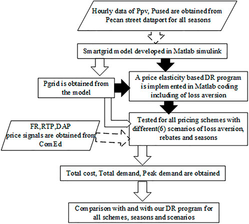
The flow diagram of the article is depicted in Figure 1. The simulation model of the proposed system is depicted in Figure 2. The model for the smart grid is based on the model developed by the Centre of Electromechanics, University of Texas (Austin), for the Pecan Street Project including some modifications (University of Texas, 2011; Dhundia, 2016). A substation is represented by a three-phase source with a Ph–Ph voltage of 13.8 kV, which is connected to a static load that is represented by a three-phase series RLC load through a cable. A three-winding residential transformer is tapped from the output of the cable.
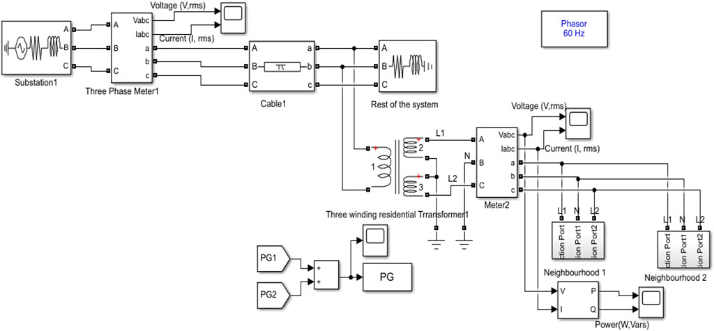
FIGURE 2. Schematic representation of a data-driven smart grid system for incorporating a DR program.
It is of 50 KVA power rating with a voltage ratio of 13.8 kV/120V–120 V. The secondary voltages of the transformer are as follows: Line 1 to Neutral= 120 V
where
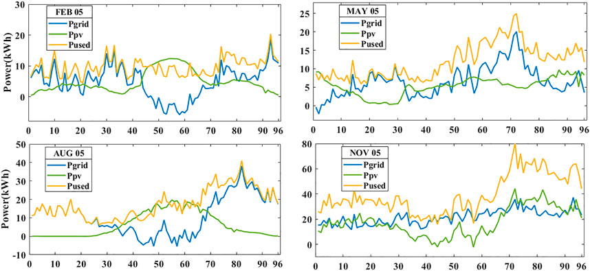
The Pecan Street dataport continuously monitors each home’s energy use and production at intervals of 1 s to 1 min and beyond. The time slots are on the horizontal axes. Here, 15 min is referred to as a single time slot. The analysis is conducted throughout each of the four seasons for an entire day. Even though we can collect data for 24 h by using a 60-min time slot, a 15-min time slot provides higher resolution data for outcome analysis. This high-resolution data shed light on the production, usage, and storage of energy.
The total power distributed among the legs is as follows:
The total power consumed by the split phase load is as follows:
where
Choosing
Then,
Each leg current phasor is calculated from the basic power equation
Then,
where [∗] = complex conjugate,
The energy supply charges (ESCs) can be calculated for different pricing schemes as follows:
For the flat-rate mechanism,
where the flat rate value is calculated as an average of the RTP pricing of the day.
For the RTP mechanism,
For the DAP mechanism,
For PTR pricing,
The standard seasonal information on Austin is categorized as summer, fall, winter, and spring. During the year of case study conduction, 20 June to 22 September is summer, 22 September to 21 December is fall, 21 December to 20 March is winter, and 20 March to 20 June is spring. A single day from each season has been considered for our analysis, that is, February 5, May 5, August 5, and November 5. The days of February and November are on the weekend. The days of May and August are on a weekday. So, the seasonal behavioral analysis can also be performed with these data. As mentioned previously,
Proposed price elasticity-based demand response program
Loss aversion
Risk aversion is the behavior of human beings (in particular, investors and consumers) in finance and economics, who strive to minimize uncertainty, if they are subjected to uncertainty. It is the reluctance of a person to participate in an unpredictable payoff scenario rather than a more predictable payoff but maybe a lower expected payoff scenario. (For example, a risk-averse investor may prefer to invest their money in a lower but guaranteed bank rate instead of a stock that may have a high return rate, which also involves an opportunity to lose value) (Mohajeryami, Schwarz, & Baboli, 2015).
The fact that losses and disadvantages have a greater effect on perceptions than benefits and advantages is a well-established behavioral fact. This results in a feature of utility that is steeper for losses than for gains. A traditional presumption that assumes a symmetry between the gain and loss value simplifies the study of an individual decision. However, it is not practical. It can, therefore, lead to over- or under-estimated assumptions. In Figure 5, a clear illustration of a value function, that can describe a broad range of outcomes, is shown. In riskless and risky situations, loss aversion is distinct. In risky situations, the value function of loss aversion is clearly steeper. The riskless scenarios include both real-time pricing and peak time discounts.
During peak hours, the utilities charge more in real-time pricing (RTP), so any load that can be shifted to peak hours appears to the consumer as a loss relative to the price of off-peak times. On the other hand, based on their load reduction, the peak time rebate (PTR) relies on rewarding the clients at the peak time. Any load that can be shifted to off-peak times is also equivalent to a gain. Their perceived value, therefore, belongs to the two opposite sides of the value function, although they are the same method, namely, shifting the flexible loads from peak to off-peak times.
Price elasticity-based demand response program:
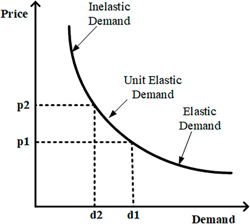
The price-elasticity curve is shown in Figure 6. When the price decreases, the demand for almost all goods and services increases. This demand shift is not linear. The non-linear demand curve can be linearized around the particular time to quantify this effect. It is regarded as the demand elasticity of the price. In other words, market elasticity is a standardized indicator of the shift in demand because price increases.
Here, E = demand elasticity; d = the value of demand; P = the price of electricity; and
(i) Some of the loads (e.g., illuminating loads) are not capable of moving from one time to the next and can only be on/off. Thus, these loads have just a single period of sensitivity and it is called “self-elasticity,” and it often has a negative value:
(ii) Such periods of consumption can be changed from high to off-peak or low periods. Such behavior is referred to as sensitivity for several periods, and “cross-elasticity” is measured. This value is positive at all times.
where
In this article, we will model the DR program depending on price elasticity and articulate how RTP, DAP, and PTR programs affect the prices and demands of electricity and how these programs can achieve the maximum customer benefit.
Modeling for a single period
Assume that
d(i) is the consumer’s demand; p(i) is the electricity spot price; I(i) is the incentive ($/kWh); and R (d(i)) is the revenue of the consumer. Also suppose that, depending on the price chosen for the incentive I(i)), the consumer changes his/her own demand from d0(i) (original value) to d(i). Thus, due to running PTR, P ($) would be as P (∆d(i)) = I(i).∆d(i) (H. Aalami et al., 2008).
Assume that the consumer’s benefit for the ith period is as shown in
where IB(i) is an incentive bonus, and in this scenario, this is a reward paid on every peak decrease in kWh. λ, It is a coefficient that represents the actual value of the incentive or reward’s nominal payment. It is believed that each person is trying to maximize their benefit. So,
Consequently,
Marginal utility is equivalent to the energy price at the optimum value. According to H. Aalami et al. (2008), for quadratic customer revenue function, the Taylor series expansion is used. So,
where d(i) represents a change from d0(i) (optimal point) in client demand. The following relation must be maintained if the initial demand is optimum prior to the introduction of the DR program.
Using (18) and the concept of demand price elasticity (12),
Plugging (21) and (22) into the extension to the Taylor series gives
It is easy to rewrite Eq. 23 as follows:
Expanding d(i) = d(i)-d0(i) and afterward relating (24) to (18) offer
So, the consumption of the consumer can also be evaluated as follows:
When I(i) is zero (i.e., no incentive award) in the aforementioned equation, d(i) would be equal to d0(i). Consequently, the price of energy would not change and the elasticity of the price will be equal to 0.
Modeling for the multi-period
The cross-elasticity between the periods i and j is described as follows:
In (28), we conclude that
The aforementioned equation shows how high the customer’s consumption should be in order to reach maximum profits in 24 h. The change in demand in Eq. 29 comes from two sources. The source is self-elasticity, expressed in the first term, and cross-elasticity, expressed in the second term, is the other source. Both price- and reward-sensitive demands are expressed in the model. In order to achieve the maximum profit in 24 h, the aforementioned equation indicates how high the consumption of the consumer should be. In the following section, we will illustrate how incentives could change the demand curve through executing FR, RTP, DAP, and PTR programs in the numerical results segment. Load profiles of the consumers are now pre-classified as low consumption, off peak and peak categories based on the different bands of power consumption and the time duration where it was obtained. The categorization of load profile is shown in Table 1. The self and cross elasticity values are fixed based on the literature and by examining with various set of values to obtain the desired outcomes. The pre-fixed self and cross elasticity values are shown in Table 2.
Analysis and discussion of results
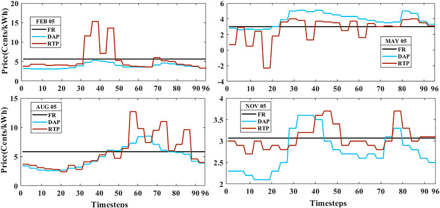
The flat rate is assumed as the average electricity price of dynamic RTP. Real-time pricing (RTP) is a service that specifically provides consumers with real-time hourly rates. In day-ahead pricing (DAP), a consumer will be told a day in advance of the price of electricity. A peak time rebate (PTR) is a program in which clients earn discounts during peak hours. Loss aversion is not considered (λ = 1) in the PTR1 program. Loss aversion is considered in the PTR2 program (λ = 0.5). Any dollar lost is considered to be twice the worth of any dollar gained. The PTR3 program is the same as PTR2, except for the doubling of the cross-elasticity constants. In PTR1,2,3 programs, the reward awarded to a client is assumed to be 2.6 times the flat rate value during peak hours. PTR4 is the same as PTR1, except that the reward being awarded is doubled, that is, 5.2 times the flat rate value.
A peak price only applies during the designated summer days, that is, June–September. Also, a very low night-time rate that applies during the five windiest months, that is, March–May and November–December (e.g., 5 August, 0.0583$, 5 May, 0.03$, and 5 November, 0.0307$). The experimental rate will be the same as the normal Austin energy rate (e.g., 5 February 0.0564$) for the remaining 3 months of January, February, and October (“ComEd’s Hourly Pricing,” 2011; McCracken and George, 2014).
Scenario 1: Impact of pricing systems on all season parameters and to illustrate the numerical results of how incentives could alter the demand curve
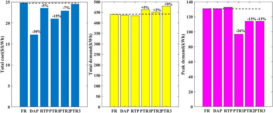
The impact of the pricing scheme on the total cost, total demand, and peak demand for all seasons has been clearly analyzed here. Initially, the analysis has been done for 5th of February. Corresponding results are tabulated in Table 3. In contrast to flat-rate pricing, the RTP scheme does not show any effect on parameters such as overall cost, total demand, and peak demand here. However, with a loss of utility income of –30% without any impact on the total demand and peak demand, the DAP scheme will have a negative impact. Compared to other pricing schemes, peak demand was reduced in the case of PTR1,2,3 (–13.06 percent to –26.13 percent). A fair amount of peak demand is reduced in PTR1, that is., -26 percent with a loss of -15 percent in utility profits. The potential to minimize the peak demand to half (-26.13 percent to -13.06 percent) and half of the utility income (15.26 percent to -7.63 percent) can be saved relative to PTR1 by considering the loss aversion (λ = 0.5) in PTR2. In conclusion, PTR2 has a moderate impact as opposed to PTR1, both in terms of peak reduction and total cost. The doubling of the cross-elasticity values in PTR3 as opposed to PTR2 indicates no effect in terms of peak reduction. However, it shows a good impact in maintaining utility in profits (-7.63% to -1.2%) and also by improving the overall carrying capacity of the demand (2.53 percent to 8.96 percent).
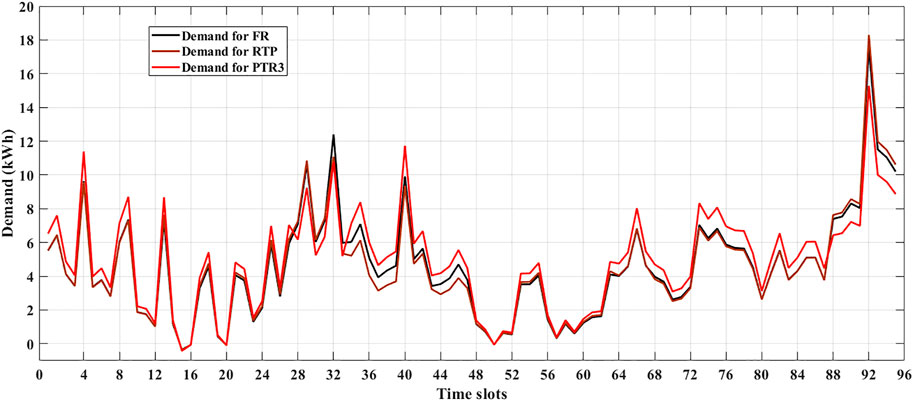
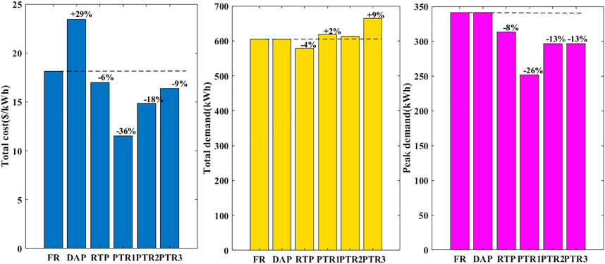
In the case of PTR4, the peak demand was drastically reduced, that is, -50 percent with a huge compromise of -64.6 percent in the total utility income, which is an adverse effect and not advisable. Of all PTR conditions, PTR3 is the best solution for peak reduction (-13 percent) without compromising on utility revenue (-1.2 percent) with load capacity improvement (9 percent) as a result of the shifting load to non-peak hours and low-price hours. Figure 7 shows the demand curve of all pricing schemes for the month of February. Figures 8, 9 shows the bar chart of all parameters and all pricing schemes for the month of February and May respectively. Figure 8 shows the bar chart of all parameters and all pricing schemes for the month of February.
Then, the analysis has been done for 5th of May, August and November. Corresponding results are tabulated in Tables 4–6 respectively. If utility income is only the criterion, DAP is considered the best in May. According to the Pecan Street report (Rate Structure Information for Time-of-Use Pricing, 2011; McCracken and George, 2014), the explanation for low income in May is due to the very low night-time rate that applies during the five windiest months (March–May and November–December). When the key concern is peak demand reduction, then PTR1 is the best option. However, because of the compromise in utility revenue (36.2 percent), it is not advisable. As far as all parameters are concerned, then PTR3 is the best choice for May with all the parameters in a moderate range. In PTR3, with a compromise of 9.5% utility revenue, 13.09% peak demand can be reduced with increased loading capability by 9.7%. In August and November, the trend of all the parameters remains the same. PTR3 is the optimal solution by keeping all parameters in concern.
Scenario 2: Impact of pricing schemes for all seasons on all parameters and contrast between seasons
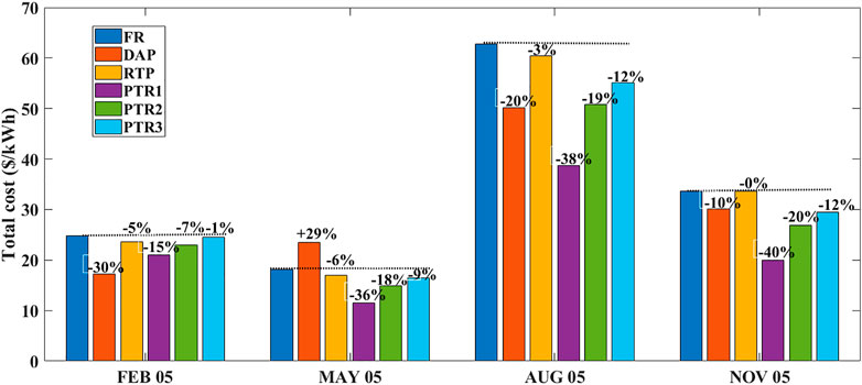
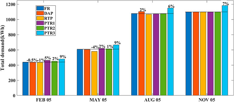
The percentage change in total cost, total demand, and peak demand is shown in bar charts for all pricing schemes in Figures 10–12, respectively. Percentage change in total cost: utility revenue has dropped in the range of 3% to 6 percent for RTP pricing in all seasons, and PTR1 for utility revenue or total cost of all seasons has dropped in the range of 15% to 40 percent. Due to λ ′s variation from 1 to 0, the total cost of PTR2 is half of PTR1. A range of 1 percent decreased to 12 percent for PTR3. Percentage change in total demand: the total demand reduction is in the range of 1 to 4 percent for RTP pricing in all seasons. The percent increase in the total demand range is 0 to +5 percent in PTR1. In PTR2, the percentage increase in the total demand range is 0 to +2%, that is, the exact half of PTR1. Percentage change in peak demand: the percentage peak decrease range for RTP is 0 to –8 percent. The percentage peak reduction range for PTR1 is 26 percent. The percentage peak reduction range for PTR2 is exactly half of PTR1 at –13 percent. The percentage peak reduction range for PTR3 is exactly the same as PTR2 at 13 percent.
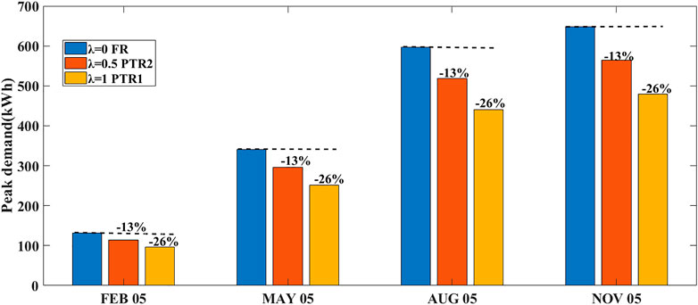
PTR1 has a positive effect on the reduction of peak demand (-26%) and the rise in total demand (0–5%). However, the reduction in utility income also had a major effect (15 to 40 percent). The credit for PTR2,3 is half the credit for PTR1 in all seasons. The cause is that λ = 0.5 is taken into account in PTR2,3, and in the demand response equation, reward 0 is replaced by 0.5*reward0. The value of λ is also expressed in the value of the credit. At the λ = 1 condition, peak demand is drastically reduced in all the seasons. Peak demand is decreased and halved at λ = 0.5 compared to λ = 1; peak demand comparison at different conditions of λ = 0(FR), 0.5(PTR2), and 1(PTR1) is shown in Figure 13.
The total demand for February and May is between 440 and 660 units. Also, the total cost is between $11 and $24 with average flat rate values of 0.0564 and 0.03. The total demand surged by almost 80% in August and November, that is, in the range of 1,050 to 1180 kwh, and cost ranges from 33 $to 50$.With the same range of the total demand, the total cost of November is almost half of that of August because the RTP price signal variation is based on the season and nature of the day. For the total demand range of ≈440units in February and ≈1,097 units in November, it charges almost in the same range of ≈24 to 30 $.
Scenario 3: Rebate or reward that has given during peak hours is 2.6 times of the flat rate (PTR4). If it is doubled, that is, the reward is equal to 5.2 times the flat rate, what will be the response?
The FEB is reviewing this situation. The corresponding changes in parameters due to doubling of rebate are tabulated in Table 7. The flat rate is 0.0564 for the FEB. The incentive is now boosted to 0.2820 (i.e., 5.2 times the flat rate) during peak hours. Peak demand is decreased by 49 percent relative to the flat rate. Also, the total demand is raised by 9%, and the utility’s total revenue is decreased by 64%. Compared to PTR1, just by changing the rebate value, much change has been observed in the percentage change in peak demand and total cost. However, it is not at all suggested as it is happening at the loss of utility revenue.
Scenario 4: Equal loss scenario and peak reduction scenario (for any season)
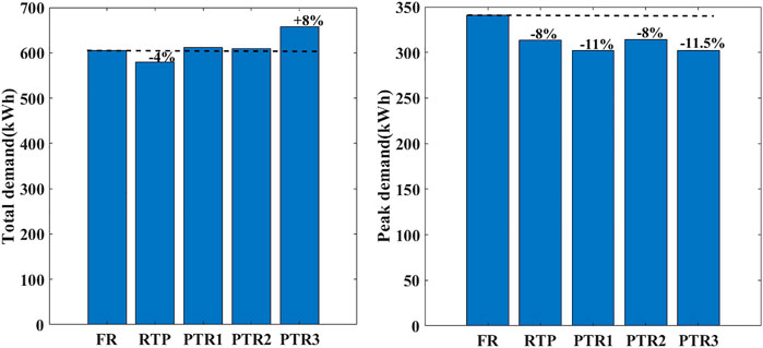
The equal loss scenario criterion is the one that evaluates how much peak reduction can be accomplished with the same amount of economic loss. In the peak reduction scenario, utilities are interested in peak reduction, regardless of the cost. The month of May is considered for analyzing these scenarios. For equal loss scenario, total demand and peak demand responses are shown in Figure 14. The implications of equal loss scenario and peak reduction scenario on the parameters are listed out in Tables 8, 9 respectively.
To retain equivalent financial loss, i.e., –6.34 percent, the PTR1 rebate is reduced to 0.0343 from $0.07845 per kWh. PTR1 can achieve a –11.4 percent peak reduction in PTR1 without taking into account the loss aversion scenario (i.e., λ = 1), compared to a –8.1 percent peak reduction in RTP. In the same way, a –7.91 percent reduction compared to RTP is accomplished by considering loss aversion in PTR2. In terms of peak reduction, PTR3 shows the same effect as PTR1, i.e., –11.51 percent. The added advantage with PTR3 is the improvement in total demand serving capability of 8.5% and peak reduction of –11.4% is attained by considering loss aversion and doubling the cross elasticity constants.
Compared to RTP, the corresponding peak reduction of 8.11 percent in PTR is achieved at λ = 0.31. RTP is responsible for utility loss of 6.34 percent for the same peak load reduction, while 11.24 percent in PTR1. Compared to RTP (4.26 percent), the total demand serving capacity is better in PTR1 (+0.7 percent). The selection of either RTP or PTR1 is solely dependent on the priority of the cost, else load demand serving capacity for the same peak reduction.
Scenario 5: For the same value of rebate, if λ is changed from 0 (FR), 0.5 (PTR2), and 1 (PTR1), then what will happen?
For the same value of rebate, change in loss aversion value effects the parameters that are shown in Table 10. For the same reward value, a decrease in peak demand is caused by λ approaching from 0 to 1. The value range is from 313.4 to 251.4 for May and 562.5 to 440.5 for August. At the same time, this allows the total demand to rise. For May, its value ranges from 579.4 to 619.6 and for August, it ranges from 1,068.3 to 1,071.3. In conclusion, the pattern of a significant reduction in peak demand and a rise in total demand is observed as λ approaches 0 to 1.
Scenario 6: For the same value of reward and λ values, are elasticity constants doubled?
For the same value of reward and λ values, but elasticity constants are doubled. Then the corresponding implications on the parameters are shown in Table 11. The total demand is significantly increased through the doubling of cross elasticity values. Their values change from 612 to 664 for May. The range is 1,073–1,149 for August. The peak demand remains unchanged for May (296–296) and August (518–518). Therefore, the peak demand has been shown to remain unaltered, and overall demand has risen by 7–8.4 percent.
Conclusion
The potential of demand response initiatives has offered new perspectives for the electricity market to participate in the process of making decisions by the clients. Time-based DR programs help enhance the indices of service and reliability. Choosing the right one among them depends on financial and technical aspects. These aspects should be integrated into the utility function of the customer. The influence of loss aversion is studied on the PTR program with different scenarios in this paper. Of all PTR conditions, without sacrificing on utility revenue with load capacity increase, PTR3 is the best option for peak reduction. There are also season-based conclusions, such as a drastic change in some parameters for a specific season or between different seasons in relation to other parameters. It also discusses the situations that make the system financially and technically unviable. The best outcomes of the peak load reduction scenario and equal loss scenario are well-explored. In conclusion, as λ approaches 0 to 1, the trend of a sharp reduction in the peak demand and an increase in the total demand is observed. The peak demand has been shown to remain constant, and the total demand has increased by doubling the cross-elasticity values.
Data availability statement
Publicly available datasets were analyzed in this study. These data can be found at: ComEd’s Hourly Pricing. (2011). Retrieved from https://dataport.pecanstreet.org/academic and from https://dataport.pecanstreet.org/academic.
Author contributions
RP has conceptualised, implemented, investigated and validated the proposed methodology for the smart grid environment. And also prepared the original manuscript. BJ has supervised the whole work and reviewed the manuscript. JI has given valuable inputs in implementing of the the work. HC has edited the manuscript for better visualization.
Acknowledgments
PR received his Bachelor of Technology degree from Kakatiya University College of Engineering, Telangana, India, in 2007. He obtained master’s degree from JNTU, Hyderabad, India. He has completed his doctoral degree from the School of Electrical Engineering, Vellore Institute of Technology, Tamil Nadu, India. He has more than 11 years of teaching and research experience in electrical engineering in reputed organizations including VIT and Ministry of Manpower, Sultanate of Oman. His research interest includes energy management, demand-side management/demand response, optimization, energy efficiency in buildings, and grid-connected PV Systems, IoT. JB (corresponding author) received his B.E. in Electrical Engineering from Manonmaniam Sundaranar University, Tamilnadu, India, in 1999, an ME in Power Systems from Annamalai University, Tamil Nadu, India, in 2002 and a PhD from Anna University, Chennai, in 2013. He has been working as an Associate Professor at Vellore Institute of Technology, Tamil Nadu, India. He has more than 19 years of experience in teaching and research. His major scientific interest is focused on power system optimization and protection, optimal location of FACTS and DG devices, renewable energy systems, and demand-side management. He has been serving as secretary for the IEEE i-PACT conference 2017, 19, and 21. IJ was born in India and received his bachelor’s degree in Electrical Engineering from The Indian Engineering College and master’s degree in Power Systems Engineering from Annamalai University with first class in 2000 and 2001, respectively. He has completed his Ph.D. degree in the Department of Electrical and Electronics Engineering, Indian Institute of Technology, Roorkee, India, in the year 2007. He is presently working as a Professor in the School of Electrical Engineering, Vellore Institute of Technology (VIT). His field of interest is unit commitment, economic dispatch, power system restructuring and deregulation, artificial intelligence applications to power system, and FACTS. CH has 2.6 years of teaching experience. He received his bachelor’s degree in Electrical & Electronics Engineering from Jawaharlal Nehru Technological University, Anantapuramu, India, and a master’s degree in Power Electronics & Drives from VIT University, Vellore, India, in 2013 and 2016, respectively. He received his Ph. D from VIT University, Vellore, India, in the year 2022. He has published various SCI, Web of Science, Springer Book Chapters, and SCOPUS indexed journals. His research interests include PV cell modeling, fuel cell modeling, soft computing, artificial intelligence, power point tracking techniques, liquid dielectrics, spectroscopy analysis, and design of high step-up dc-dc converters for electric vehicle application.
Conflict of interest
The authors declare that the research was conducted in the absence of any commercial or financial relationships that could be construed as a potential conflict of interest.
Publisher’s note
All claims expressed in this article are solely those of the authors and do not necessarily represent those of their affiliated organizations, or those of the publisher, the editors, and the reviewers. Any product that may be evaluated in this article, or claim that may be made by its manufacturer, is not guaranteed or endorsed by the publisher.
References
Aalami, H. A., Pashaei-Didani, H., and Nojavan, S. (2019). Deriving nonlinear models for incentive-based demand response programs. Int. J. Electr. Power & Energy Syst. 106, 223–231. doi:10.1016/j.ijepes.2018.10.003
Aalami, H., Yousefi, G. R., and Parsa Moghadam, M. (2008). “Demand response model considering EDRP and TOU programs. Transmission and Distribution Exposition Conference,” in 2008 IEEE PES powering toward the future. doi:10.1109/TDC.2008.4517059
Abapour, S., Mohammadi-Ivatloo, B., and Tarafdar Hagh, M. (2020). Robust bidding strategy for demand response aggregators in electricity market based on game theory. J. Clean. Prod. 243, 118393. doi:10.1016/j.jclepro.2019.118393
Ajoulabadi, A., Ravadanegh, S. N., and Mohammadi-Ivatloo., Behnam (2020). Flexible scheduling of reconfigurable microgrid-based distribution networks considering demand response program. Energy 196, 117024. doi:10.1016/j.energy.2020.117024
Chai, Y., Xiang, Y., Liu, J., Gu, C., Zhang, W., and Xu, W. (2019). Incentive-based demand response model for maximizing benefits of electricity retailers. J. Mod. Power Syst. Clean. Energy 7 (6), 1644–1650. doi:10.1007/s40565-019-0504-y
ComEd’s Hourly Pricing (2011). ComEd’s hourly pricing. Retrieved from Available at: https://dataport.pecanstreet.org/academic.
Hosseini Imani, M., Niknejad, P., and Barzegaran, M. R. (2019). Implementing Time-of-Use Demand Response Program in microgrid considering energy storage unit participation and different capacities of installed wind power. Electr. Power Syst. Res. 175, 105916. doi:10.1016/j.epsr.2019.105916
Jiang, J., Kou, Y., Bie, Z., and Li, G. (2019). Optimal real-time pricing of electricity based on demand response. Energy Procedia 159, 304–308. doi:10.1016/j.egypro.2019.01.011
Lu, R., and Hong, S. H. (2019). Incentive-based demand response for smart grid with reinforcement learning and deep neural network. Appl. Energy 236 (2018), 937–949. doi:10.1016/j.apenergy.2018.12.061
McCracken, B., and George, T. (2014). Pecan street smart grid demonstration project interim Technology performance report.
Mohajeryami, S., Schwarz, P., and Baboli, P. T. (2015). Including the behavioral aspects of customers in demand response model: Real time pricing versus peak time rebate. North American Power Symposium. doi:10.1109/NAPS.2015.7335116NAPS
Monfared, H. J., Ghasemi, A., Loni, A., and Marzband, M. (2019). A hybrid price-based demand response program for the residential micro-grid. Energy 185, 274–285. doi:10.1016/j.energy.2019.07.045
Rajendhar, P., and Belwin Edward, J. (2019). “Application of demand response and co-simulation approach for renewable integrated home energy management system: A review,” in IET generation, transmission & distribution (United Kingdom: Wiley). doi:10.1049/iet-gtd.2018.5791
Rate Structure Information for Time-of-Use Pricing (2011). Rate structure information for time-of-use pricing. Retrieved from Available at: https://www.pecanstreet.org/wp-content/uploads/2011/07/Pricing-trial-rate-overview.pdf.
Residential data page of Pecan street data port (2022). Residential data page of Pecan street data port. Retrieved from Available at: https://dataport.pecanstreet.org/academic.
Sharifi, R., Fathi, S. H., Anvari-Moghaddam, A., Guerrero, J. M., and Vahidinasab, V. (2018). An economic customer-oriented demand response model in electricity markets. Proc. IEEE Int. Conf. Industrial Technol., 1149. –1153. doi:10.1109/ICIT.2018.8352340
Shi, Q., Chen, C. F., Mammoli, A., and Li, F. (2020). Estimating the profile of incentive-based demand response (IBDR) by integrating technical models and social-behavioral factors. IEEE Trans. Smart Grid 11 (1), 171–183. doi:10.1109/TSG.2019.2919601
University of Texas, C. for electromechancis (2011). Simulink smartgrid simulation 1: The basics. Retrieved from Available at: https://www.youtube.com/watch?v=UvOJh534cok&t=228s.
Nomenclature
Acronyms
DR demand response
FR flat rate
RTP real-time pricing
DAP day-ahead pricing
PTR peak time rebate
IBDR incentive-based demand response
ESC energy supply charge
Variables
E demand elasticity
d value of demand
p price of electricity
λ coefficient that represents the actual value of the incentive or reward’s payment
Indices
i,j time periods
Keywords: demand response (DR), electricity market, loss aversion, price elasticity of demand, peak time rebate (PTR), smart grid
Citation: Puppala R, Jeyaraj BE, Isaac JR and CH HB (2023) Framework for smart grid to implement a price elasticity-based peak time rebate demand response program. Front. Energy Res. 10:1079695. doi: 10.3389/fenrg.2022.1079695
Received: 25 October 2022; Accepted: 15 November 2022;
Published: 04 January 2023.
Edited by:
Sarat Kumar Sahoo, Parala Maharaja Engineering College (P.M.E.C), IndiaReviewed by:
Sakda Somkun, Naresuan University, ThailandSuresh Kumar Velu, Thiagarajar College of Engineering, India
Saroj Padhan, Parala Maharaja Engineering College (P.M.E.C), India
Copyright © 2023 Puppala, Jeyaraj, Isaac and CH. This is an open-access article distributed under the terms of the Creative Commons Attribution License (CC BY). The use, distribution or reproduction in other forums is permitted, provided the original author(s) and the copyright owner(s) are credited and that the original publication in this journal is cited, in accordance with accepted academic practice. No use, distribution or reproduction is permitted which does not comply with these terms.
*Correspondence: Belwin Edward Jeyaraj, amJlbHdpbmVkd2FyZEB2aXQuYWMuaW4=
 Rajendhar Puppala
 Belwin Edward Jeyaraj
 Jacob Raglend Isaac
 Hussaian Basha CH