Distributed algorithm without iterations for an integrated energy system

Existing energy management methods for integrated energy systems are mostly in distributed communication and computation now, need a large number of iterations, and each time of iteration needs lots of communication and computation. For this reason, on one hand, the iteration may cause energy-delay. On the other hand, iteration will significantly increase the communication and computation burden. The integrated energy systems contain a variety of devices and energy resources (including renewable energy resources), so the communication and computation burden is already very high. If the communication and computation cannot be solved very well, the cost functions of each device need to be much easier to ensure the operation of the system and their systematic error will be much larger. For this reason, the result of optimization will be much worse because of the accuracy of cost functions. The greatest challenge of this issue is to establish an algorithm without iteration. For handling this issue, first, we adopt the theoretical demonstration to prove that if all prices of all devices are the same, the optimization will be realized and the instantaneous price is the one-order derivative. (we assume the relationship between the operating cost and the energy flow of each device as the convex cost functions.) Second, we reshape all cost functions. Third, we change the function to the total of the foregoing functions in the directed annular path and adopt the total function of the hole system to solve the energy price. Last, we use the price to ensure their operating condition. Our theoretical demonstration has already proved the optimization, convergence, the plug and play performance, scalability, and the emergency scheduling performance of the annular partial differential algorithm (APDA).

1 Introduction

Recently, there were several papers on the concept of “integrated energy system (IES)” for handling problems related to utilizing sustainable and environmentally friendly renewable energy resources, renovating the energy utilization model, enhancing energy management, and securing system control (Wang et al., 2021; Zhou et al., 2021; Chen et al., 2022). The most prominent development regarding the IES is a framework that includes various energy types. During the transition from traditional single-energy systems to an IES, the most important issue that should be revisited is how to maximize social profits (Liu et al., 2022a). Accordingly, the energy management issue, which is one of the fundamental issues in power systems (Yang et al., 2022), should be revisited to achieve the envisioned IES concept.

Fundamentally, energy management is formulated as an optimization problem. Numerous methods have been adopted to address the optimization problem, which can be classified into two main categories: centralized approaches (CAs) and distributed approaches (DAs). The CA optimally dispatches various energy resources in different areas by running an integrated economic dispatch center over the entire IES. However, an IES is typically composed of too many distributed areas that may be operated by various energy operators; therefore, a centralized solution for the IES is impractical owing to both technical and administrative reasons. In addition, the CA depends on a strong centralized control center and numerous communication paths from that center, which can sharply increase computational costs and the likelihood of single-point failures. Moreover, the CA cannot ensure user privacy. To address these shortcomings, with the development of multi-agent systems, numerous scholars have adopted DAs to replace CAs. The design of a DA is inspired by the multi-agent theory and edge computing methods in the fields of computing and blockchain (Wei et al., 2021; Feng et al., 2022a; Feng et al., 2022b; Liu et al., 2022b; Mao et al., 2022; Wei et al., 2022). DAs aim to achieve multi-area integrated optimality in a distributed and coordinated fashion without revealing the private information regarding each area. Compared with CAs, DAs exhibit better robustness (Xing et al., 2015; Hua et al., 2018; Xu et al., 2019), scalability (Binetti et al., 1720; Huang et al., 2022; Kirli et al., 2022), resilience (Abessi and Jadid, 2021; Guo et al., 2021; Mishra et al., 2022), and privacy protection (Zhou et al., 1667), (Zhou et al., 2020). Zhang et al. (2017) proposed a distributed consensus algorithm that can be applied to energy management in a fully distributed manner for the first time. The novel distributed algorithm introduced in Chen et al., (2015) does not require projection and can control the underlying power flow. In addition, many scholars have integrated event-triggered theory with DAs to reduce redundant communications in the IES. Tan et al. (2021) and Tan (2022) investigated asynchronous communication DA systems with partial inputs. Liu et al. (2021) examined an event-triggered system with bipartite consensus-quantized control. From these studies, we can conclude that the DA is better suited to energy management because it disintegrates global computation into local computation and assigns the energy management problem to the energy subsystem and distributed energy device, which uses only local communication, computation, and control to achieve optimal operation. Ma et al. (2021) proposed a three-step-based graph partitioning algorithm to divide a power network into several groups according to the characteristics of power flow to adjust bus among the groups. He et al. (2017) studied the group work and big data and combined the power flow analysis and fault detection for the first time. However, the fault detection does not only fit for electrical power system, but the pipeline network also needs fault detection. Hu et al. (2022) studied the fault detection of the small leak location for intelligent pipeline. Ma et al. (2022) proposed a dual-predictive control method to handle the error issue. Chang et al. (2021) had already modeled the network constraint to avoid the power flow violating the limit.

The main idea behind the existing multi-agent theory and edge computing studies is that to optimally control a complex and large industrial system, the large system should be divided into small systems, which should be appropriately adopted to optimally control the large system. This approach is similar to dividing the smart grid into microgrids and dividing the multi-agent system into agents. Therefore, the IES must be divided as well. For handling this issue, Yang et al. (2020) proposed the concept of “we-energy” to divide an IES. As a subunit of the IES, we-energy is a small independent energy system coupled with various energy sources. These small energy systems are connected to each other through energy ports to form an IES. In addition, we-energies are significantly different from microgrids because they are deeply coupled systems of information, physics, energy, and economics. We-energy can play various roles in an IES, including but not limited to energy manufacturing, energy consumption, energy conversion hubs, and energy store hubs. In summary, this study adopts we-energy as a subsystem of IESs.

Although DA applications in IESs have already been developed significantly, these existing methods still have many limitations. First, an excessive number of iterations can aggravate the communication and computational burden. The reason for this is that the DA only disperses the communication and computational burden from the control center to the hole system; however, the total communication and computational burden remains exceedingly large because the existing DA approaches require iterations on many occasions. If the iterations waste too much time, the communication and computation costs become significant and the time wasted by the iteration may cause an energy delay. Second, the adoption of DAs in energy management is dependent predominantly on assumptions regarding the operating conditions of devices in an IES and well-tuned algorithm parameters. However, tuning certain parameters is extremely challenging. Third, except for several finite-step distributed algorithms, (Zhao et al., 2014); (Guo et al., 2017), most traditional decomposition methods and distributed algorithms are asymptotically convergent, resulting in a trade-off between the accuracy of a given algorithm and number of iterations (Lai et al., 2017).

Although existing DAs can disperse the communication and computation burden from the control center to every we-energy, the communication and computation burden is still in the IES. In addition, compared with traditional electrical power systems, the IES contains more energy types, more energy resources, and more energy loads. So the complexity of the IES is much higher than that of traditional electrical power systems, which will significantly increase the communication and computation burden. Also, that burden will do great harm to the IES. On one hand, if that burden is too large, the IES needs to consume enormous costs on communication and computation. Traditional electrical systems only dispatch energy costs and ignore communication and computation costs. However, the communication and computation cost is also very high, especially in complicated IESs. On the other hand, too much communication and computation will consume too much time. In a power–heat–gas IES, the time scale of power is much shorter than that of heat and gas. However, the complex of heat and gas in energy quality ( temperature of the water and calorific value of gas) and energy transmission is much higher than that of power. In the traditional electrical power system, we only need to dispatch power, so energy management is not very slow so that power may not be a delay. However, in the IES, we need to communicate and compute power, heat, and gas. So, the power time delay will happen more frequently.

To overcome these challenges, it is necessary to develop a distributed algorithm without iterations as it can considerably reduce communication and computational costs, has better accuracy, and is insensitive to parameters and initial values. First, each iteration needs to communicate and compute, and an iteration usually takes significant time. Consequently, the communication and computational costs in an algorithm with iterations is one hundred times less than those of an algorithm without iterations. Second, traditional algorithms with iterations are asymptotically convergent, which results in a trade-off between accuracy and number of iterations. Because the IES is a large system, a few unfit parameters can result in a strong energy mismatch. Third, the algorithms with iterations are sensitive to parameters and initial values because the result may lead to oscillation or divergence. However, the algorithm without iterations does not have this disadvantage.

To address these problems, we propose an algorithm without iterations called the annular partial differential algorithm (APDA) in this study. First, we depict a theoretical demonstration to prove that if all devices are priced the same, optimization can be realized, and instantaneous price becomes a one-order derivative. Second, we reshape all cost functions. We set the independent variable to the first derivative and dependent variable to the energy value. Third, we changed the function to the total of the foregoing functions in the directed annular path. Each agent must be computed only once. Fourth, we adjusted the total function of the hole system to set the energy price. Finally, we transmit the energy prices to all devices, and the devices can use this price point to ensure their operating conditions. Our theoretical demonstration has already proved that APDA reliably attains the optimal operating condition for an IES. The key contributions of this study are as follows:

1) APDA can avoid energy delays and significantly reduce the communication and computational burden of the IES. In existing DA applications, each iteration requires communication and computation. However, APDA does not require iterations; therefore, the communication and computational burden will be much less. In addition, the algorithm without iteration will be much quicker; thus, an energy delay because of the slow algorithms will never occur.

2) The APDA is far more accurate than existing algorithms. Existing decomposition methods and distributed algorithms are asymptotically convergent, resulting in a trade-off between the accuracy of a given algorithm and the number of iterations. However, the APDA does not suffer from this problem because it can accurately determine the optimization result in one communication and computation iteration.

3) The APDA does not depend on suitable parameters or initial values. Existing algorithms are sensitive to parameters and initial values because the results may lead to oscillation or divergence. However, the APDA does not suffer from this disadvantage.

4) Privacy protection in the APDA is much better than that in existing algorithms. Although existing distributed methods can protect user privacy to a certain degree, there are still some ratios, power outputs, or estimated prices that must be shared among neighboring agents. However, the APDA can protect all data, including the information presented below, among neighboring agents. In the APDA, there are no neighbor agents because all data in the APDA are cryptographic, and neighbor agents are meaningless.

Table 1 summarizes the performance of the APDA and traditional methodologies to underline the contribution of this study. Table 2 summarizes the methods used in the APDA and whether the innovation of this study is original or not. The non-iterative mechanism of the APDA is summarized as follows:

TABLE 1

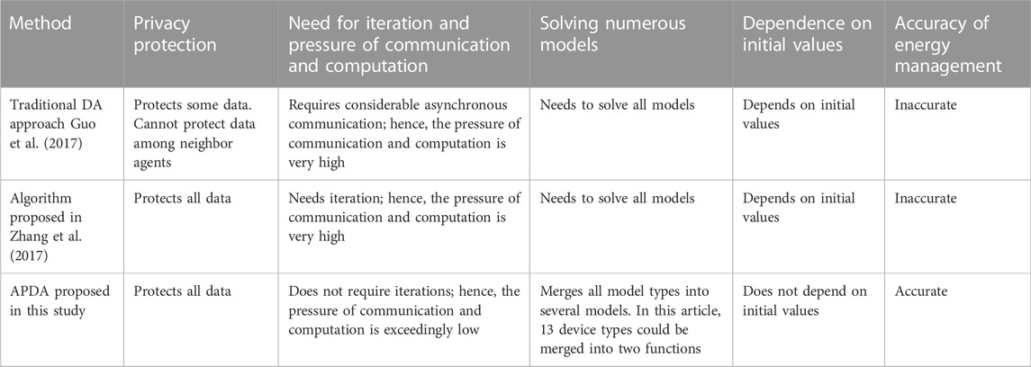
TABLE 1. Contributions of different methods.

TABLE 2

TABLE 2. Innovation of this study.

The APDA transforms all cost functions into another function type. The independent variable of this function is the first-order differential, and the dependent variable is energy flow. The APDA accumulates the differentials of all orders into new functions via an annular communication path. The annular path can be used to ensure that the APDA can sum all differentials in a distributed manner. Accordingly, the high computational and communication pressure on the control center is overcome. The control center can utilize the total of these differentials to restore the hole functions. The independent variable of this function is the first-order differential, and the energy mismatch is the dependent variable. The number of hole functions corresponds to the number of energy types. The control center uses each hole function to set an independent variable for each energy type. These independent variables were regarded as the energy prices of the corresponding energy types. The control center relays the prices of each energy source using the communication path, and each device adjusts the operating conditions according to these prices. Under these circumstances, convergence and optimization are satisfied, and iteration is not required. A detailed introduction and proof of the APDA are presented below.

The presented APDA can significantly speed up the optimization algorithm and protect the user privacy effectively. Therefore, it is suitable for the IES, which requires high speed and good privacy protection. However, the APDA requires synchronous communication and large-scale communication simultaneously. Some changeable IESs are unfit because they require frequent dispatches. In addition, the APDA can only handle convex optimization, and an IES with non-convex devices is unsuitable for it. Therefore, the IES approaches depicted in Yang et al. (2020) and Tan and Li (2022) are suitable for the APDA, while the IESs presented in Wang et al. (2021) and Feng et al. (2022b) are not.

2 Models of IESs

The devices in we-energies are listed in Table 3.

TABLE 3

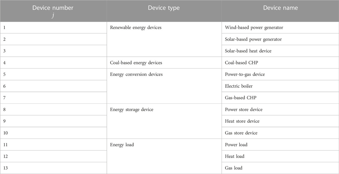
TABLE 3. Devices in each we-energy.

Here, $j$ denotes the number of devices and $i$ denotes the number of we-energies. The IES has three types of energy: power, heat, and gas. The vector $\left\{X_{i,j}\in R^3\left|i=1\right.,\dots ,n+1;j=1,\dots ,12\right\}$ has three dimensionalities that indicate the operating conditions (power–heat–gas input or output) of devices. The element $x_{i,j}^m$ represents the $m$-th element in that vector. The power–heat–gas energy flow rate are $x_{i,j}^1$, $x_{i,j}^2$, and $x_{i,j}^3$, respectively. Additionally, the IES has a centralized power plant. Owing to the aforementioned reasons, the centralized power plant cannot be settled in we-energies. In addition, the centralized power plant should not be CHP because heat cannot be transmitted over long distances. The energy in the centralized power plants is exceedingly large. Thus, we can ignore the heat demand near the plant.

2.1 Models and limits of the IES

Devices in the IES can be divided into two types: certain and uncertain devices. Devices that can be controlled are certain devices; for example, CHP and energy conversion devices are certain devices, whereas devices that cannot be controlled are uncertain devices. In the IES, the uncertain devices are renewable energy devices and terminal energy loads. It should be noted that uncertain devices do not have any operating cost functions because the operating cost for energy devices and terminal energy loads is considerably low. These devices have only an energy input or output value $x_{i,j}^m$. The limits for uncertain devices are

$\left\{x_{i,j}^m\in \left[0,x_{i,j}^{m-up}\right]\right\}.(1)$

$x_{i,j}^{m-up}$ represents the operating limit. Because the performance of uncertain devices including but not limited to lines and transformers is not infinite, we need to establish an operating limit.

The operating cost function and limits of CHP are

$C_{i,j,t_k}={\mathrm{a}}_{i,j}{x}_{i,j}^{1^2}+{\mathrm{b}}_{i,j}{x}_{i,j,t_k}^1+{\mathrm{\alpha }}_{i,j}{x}_{i,j,t_k}^{2^2}+{\mathrm{\beta }}_{i,j}{x}_{i,j,t_k}^2+{\chi }_{i,j}(2)$

where ${\mathrm{a}}_{i,j},{\mathrm{b}}_{i,j},{\mathrm{\alpha }}_{i,j},{\mathrm{\beta }}_{i,j}$, and ${\chi }_{i,j}$ represent constants and ${\mathrm{a}}_{i,j}$ is positive. We regard the energy conversion efficiency of gas or coal to power and heat as 100%. The constant values in Equation 2 and other equations determine the character of devices. The constant values affect the relationship between the operating cost and the rate of energies. The main motivation of the APDA is the scalability because the APDA suits all kinds of convex functions. How to match cost functions is not the emphasis of the APDA.

The limits are

$-P_{i,j}^{\text{ramp}}\le x_{i,j,t_k}^1-x_{i,j,t_{k-1}}^1\le P_{i,j}^{\text{ramp}},(3)$

${\mathrm{d}}_{i,j}{x}_{i,j,t_k}^1+{\mathrm{e}}_{i,j}{x}_{i,j,t_k}^2+{\mathrm{f}}_{i,j}\ge 0,(4)$

${\mathrm{d}}_{i,j}{x}_{i,j,t_k}^1+{\mathrm{e}}_{i,j}{x}_{i,j,t_k}^2\le {\mathrm{g}}_{i,j},(5)$

$\left\{x_{i,j}^m\in \left[x_{i,j}^{m-\text{down}},x_{i,j}^{m-up}\right]\right\}.(6)$

$x_{i,j}^{m-\text{down}}$ and $x_{i,j}^{m-up}$ indicate the operating limits of CHP, and $P_{i,j}^{\text{ramp}}$ denotes the ramp limit of power. Because the output of’ CHP cannot change too fast, we should add a ramp limit. However, we only consider the ramp limit of power because the time-scale of heat is exceedingly large. In addition, the CHP also has a maximum operating limit and a start–stop limit. The reason for the maximum operating limit is very easy to understand. However, what is the reason for the start–stop limit? If a CHP stops operating, it is too hard to restart it. So we need to establish a start–stop limit to keep the CHP in operation. Zhang et al. (2017) have already shown that the maximum operating limit and the start-–stop limit for CHP should be linear as in (4) and (5). ${\mathrm{d}}_{i,j},{\mathrm{e}}_{i,j},{\mathrm{f}}_{i,j}$, and ${\mathrm{g}}_{i,j}$ are positive constants. In addition, because the power and heat output transmission of CHP is not infinite, we establish limit (6), and $x_{i,j}^{m-\text{down}}$ and $x_{i,j}^{m-up}$ indicate the transmission limits of CHP.

Natural gas is a fossil fuel; hence, we cannot produce it. Gas price is decided by other departments, and not by the IES.

The model and limits of energy storage devices are

$\begin{array}{l}{O}_{i,j,t_{k}i,t}^m={\mathrm{a}}_{i,j}{x}_{i,j,t_k}^{m-S}\left(x_{i,j,t_k}^{m-S}-{\mu }_{i,j}^m\right)+{\mathrm{b}}_{i,j}\\ C=O_{i,j,t_{k}i,t}^m-O_{i,j,t_{k}i,t-1}^m\end{array},(7)$

It is worth noting that there are two energy values in the energy storage device. One is the energy that is stored in the energy storage device, for which we use $x_{i,j,t_k}^{m-S}$ to express, and the other is the energy output (input) to (from) the IES, for which we adopt $x_{i,j,t_k}^m$ to express. In addition, because if the energy in the storage device is too much or too little will reduce the service life of the device, each energy storage device has an optimization store value, and we adopt $O_{i,j,t_{k}i,t}^m$ to express the optimization of energy storage value. So, the cost of the energy storage device is the loss of store optimization. ${\mathrm{a}}_{i,j},{\mu }_{i,j}^m$, and ${\mathrm{b}}_{i,j}$ are constants and ${\mathrm{a}}_{i,j}$ is negative. Thus, we obtain

$x_{i,j,t_k}^m=x_{i,j,t_{k-1}}^{m-S}-x_{i,j,t_k}^{m-S}.(8)$

The limits are

$-x_{i,j}^{m^{\mathrm{in}-\mathrm{S}\mathrm{D}}}\le x_{i,j,t_k}^m\le x_{i,j}^{m^{\mathrm{out}-\mathrm{S}\mathrm{D}}}|x_{i,j}^{m-S-\min }\le x_{i,j,t_k}^{m-S}\le x_{i,j}^{m-S-\max }.(9)$

Not only the energy exchanged from the IES but also the energy stored in the energy storage devices has maximum and minimum limits, so there are four limits in one energy storage device. $x_{i,j}^{m_{\mathrm{i}\mathrm{n}-\mathrm{S}\mathrm{D}}}$ and $x_{i,j}^{m_{\mathrm{o}\mathrm{u}\mathrm{t}-\mathrm{S}\mathrm{D}}}$ are the energy input and output limits, respectively; and $x_{i,j}^{m-S-\min }$ and $x_{i,j}^{m-S-\max }$ indicate minimum and maximum energy store limits, respectively.

Furthermore, there is a coupling item of energy load because one load can choose more than one energy to realize its function. In this study, we considered that the power to gas devices and electric boilers are supplied by energy transformation devices that can change energy loads. It is worth mentioning that the energy transformation devices need to satisfy the energy input required to be a price-changeable energy, so gas-based CHPs are not classified under such devices. The energy load changing and its cost is given as

$∆x^a=-\eta \times ∆x^b\left|C=\mathrm{w}\times ∆x^a\right..(10)$

Essentially, we can adopt load of energy a to replace load of energy b. The energy conversion efficiency is $\eta$, and the operating cost price is $\mathrm{w}$.

The cost function of the equivalent gas producer is

$C_{i,t}^{\text{DGP}}={\mathrm{a}}_{i,t}^{\text{DGP}}{G}_{i,t}^{\text{DGP}\mathit{2}}+{\mathrm{b}}_{i,t}^{\text{DGP}}{G}_{i,t}^{\text{DGP}}+{\mathrm{c}}_{i,t}^{\text{DGP}}.(11)$

How to model the network limits? Because the information and the energy flow are disconnected in the APDA and the privacy protection in the APDA is entire, the energy flow in the APDA can choose every path, and each we-energy can link to every other we-energies. In other words, the adjacency matrix of the APDA is an all-one matrix. For this reason, the energy flow in the APDA is more free than that in existing distribution methods, so the possibility of energy violating the limit is much less in the APDA than in other distribution methods. The only two possibilities of that harm are as follows. on one hand, if the hole energy flow in the hole IES is very large, all networks cannot handle the energy, and the energy violating the limit may happen. On the other hand, if the energy input or output in one we-energy is large, the energy transmission will go wrong. The complex network can change the energy flow to another path in the network, but if too much energy will transmit from (to) one we-energy, the complex network will be meaningless. The two cases can be handled together. We can establish an energy output or input limit for each energy because the energy that the IES network can contain is much larger than the total absolute value of each we-energy limit. In addition, because the operation of each device is dependent on the energy price, we can change the energy limit to the price limit of each we-energy. Each we-energy will compute its two price limits by the island model before energy management. Then, if the dispatch result of the price is beyond the energy limit, the we-energy will stop dispatch and operate by its price limit. The IES will consider it as a device that cannot respond to dispatch.

3 APDA and its advantages

Notably, the APDA is scalable. Models discussed previously only serve as examples. However, all types of IESs with convex models are suitable for the APDA. To this end, this study introduces the application of the APDA to all convex IES models except for the proposed model.

3.1 Communication path

First, the communication path of the APDA is not a traditional centralized communication path or traditional distributed communication path. It is an annular-directed communication path from Zhang et al. (2017) shown in Figure 1A–C, which illustrates the traditional centralized and distributed IES. There are several advantages of the annular-directed communication path, of which the biggest advantage is that it is compatible with the APDA. The difference between the three communication paths is listed in Table 4.

FIGURE 1

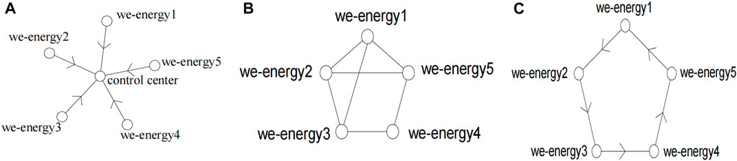
FIGURE 1. (A). Traditional centralized IES (B). Traditional distributed IES (C). Annular-directed IES.

TABLE 4

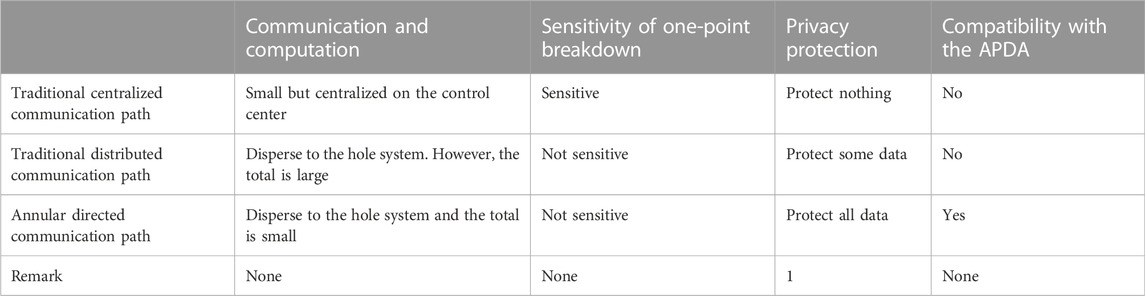
TABLE 4. Devices in each we-energy.

Remark 1: In traditional research energy ratios, energy input or output and energy prices had to be known among neighboring agents; hence, they could not completely protect privacy. However, in the annular communication in the APDA, all data are cryptographic, which ensures that all data are completely protected even if among neighbor agents, no information is known by each other. The reason behind this will be introduced in the proceeding sections.

Privacy protection in the IES means that designers should make information, including but not limited to energy input, energy output, energy store values, and parameters in one we-energy, unknown to other we-energies because they may be business competitors. The APDA only needs to transmit some parameters, so protecting parameters is the content of privacy protection in the APDA. Existing methods established some neighbor agents and then transmitted data between them and did not transmit data to non-neighbor agents to protect privacy. Although privacy protection in existing studies can protect users’ privacy to a certain degree, private data are still obtained by neighbor we-energies. However, in the annular-directed communication path of Figure 1C, privacy protection can protect all data, including data between neighbor agents. In the annular-directed communication path, all we-energies can only get the summation of corresponding parameters before them in the annular path so they do not know the parameter values in every previous we-energy. Furthermore, we will establish some fictitious parameter values to protect the privacy of the first agent. By this method, all privacy will be protected so there are not any neighbor agents. It is worth noting that the cyber information communicating path for the APDA is a simple annular path. However, the energy transmitting path is not the circle. The cyber information communicating path only transmits information but not energy because if energies transmit in a simple circle, the energy transmission cost will be very high. After the running of the APDA, the balance of all energies will be realized. Then, how to transmit corresponding energies to corresponding we-energies will be an easy elementary math problem that does not need any algorithms. So, this article does not discuss the energy-transmitting path. However, the equivalent gas producer does not have the gas limit because it does not belong to the IES, although we regard it as a we-energy. It can transmit gas to corresponding places directly.

3.2 Model adjusting

For some IESs with a strong ability for computation and communication, adopting their model may be the best choice. However, for some IESs with a weak ability for computation and communication, the APDA needs to reduce the order of models to reduce communication and computation by using the method in Lai et al. (2017). We assume that the model order limit of the IES is 2.

If the function $\mathrm{f}\left(\mathrm{x}\right)$ is a polynomial function but the order is too high, we can adopt Chebyshev approximation to reduce the order, as shown below.

Herein, we introduce how one order can be reduced. If several orders need to be reduced, the APDA will reduce the order repeatedly until the order meets the standard. We assume that there is only one independent variable in the function. If there is more than one independent variable, the APDA will handle them sequentially.

$\begin{array}{l}{\mathrm{T}}_0\left(\mathrm{x}\right)=1;\\ {\mathrm{T}}_1\left(\mathrm{x}\right)=\mathrm{x};\\ {\mathrm{T}}_2\left(\mathrm{x}\right)=2{\mathrm{x}}^2-1;\\ \dots \dots \\ {\mathrm{T}}_{\mathrm{n}+1}\left(\mathrm{x}\right)=2\mathrm{x}{\mathrm{T}}_{\mathrm{n}}\left(\mathrm{x}\right)-{\mathrm{T}}_{\mathrm{n}-1}\left(\mathrm{x}\right)\end{array}(12)$

$\mathrm{P}\left(\mathrm{x}\right)=\mathrm{f}\left(\mathrm{x}\right)-\frac{\mathrm{a}}{2^{\mathrm{n}-1}}{\mathrm{T}}_{\mathrm{n}}\left(\mathrm{x}\right),$

where $\mathrm{f}\left(\mathrm{x}\right)$ represents the primitive function; $\mathrm{P}\left(\mathrm{x}\right)$ represents the new function; and $\mathrm{a}$ indicates the coefficient of the highest order in $\mathrm{f}\left(\mathrm{x}\right)$.

If the function $\mathrm{f}\left(\mathrm{x}\right)$ is an exponential function or another convex function that is not primitive, we can fit it into a primitive function and handle it as a primitive function using the Lagrange interpolation polynomial, as shown below.

First, we select $\text{three}$ points on $\mathrm{f}\left(\mathrm{x}\right)$, and we use independent variables to solve function variables. Subsequently, we solve $\mathrm{f}\left(\mathrm{x}\right)$ as

${\mathrm{w}}_{\mathrm{k}}\left(\mathrm{x}\right)={\displaystyle \prod }_{\mathrm{m}=0}^{\mathrm{k}-1}\left(\mathrm{x}-{\mathrm{x}}_{\mathrm{m}}\right),(13)$

${\mathrm{L}}_{\mathrm{k}}\left(\mathrm{x}\right)={\displaystyle \sum }_{\mathrm{p}=0}^{\mathrm{k}}{\mathrm{y}}_{\mathrm{p}}\frac{{\mathrm{w}}_{\mathrm{k}+1}\left(\mathrm{x}\right)}{\left(\mathrm{x}-{\mathrm{x}}_{\mathrm{p}}\right){\mathrm{w}}_{\mathrm{k}+1}^{\prime }\left({\mathrm{x}}_{\mathrm{k}}\right)},(14)$

where $\left(x_m,y_m\right)$ represents a point on $f\left(x\right)$; $L_k\left(x\right)$ represents the new polynomial function.

All theories about model adjusting can be found in Ma et al. (2022). Additionally, model adjusting is rarely observed. In most cases, models can satisfy the standard of the IES because the APDA can substantially reduce the communication and computational pressure.

Second, we solve the first-order partial differentials of the cost functions of each type of energy (considering other energy types as constants). Accordingly, we solve their inverse functions. These functions are named as ${\mathrm{f}}_{\mathrm{w}}\left(\mathrm{x}\right),\left(\mathrm{w}\subset \left\{\mathrm{1,2,3},\dots \right\}\right)$. The independent variables are the first-order partial differentials and the dependent variables are energy values. There may be more than one ${\mathrm{f}}_{\mathrm{w}}\left(\mathrm{x}\right)$ in one device. The number of ${\mathrm{f}}_{\mathrm{w}}\left(\mathrm{x}\right)$ indicates the energy types in the devices. Moreover, some devices do not have cost functions. Their operating conditions are unchangeable. Therefore, they cannot solve first-order partial differentials. The ${\mathrm{f}}_{\mathrm{w}}\left(\mathrm{x}\right)$ values of such devices are constant functions; the constant values represent their operating conditions. Additionally, we do not consider the energy transmission devices in this step. It is worth mentioning that the APDA must first reduce orders before changing function shapes. This is because if function shapes are changed before reducing orders, the errors will be much larger. Furthermore, this study shows only the circumstance that the order limit is 2. However, in practice, the order limit can be any value owing to the different performances of energy routers.

It is worth mentioning that if the order limit of $C\left(x\right)$ is 2, then the high-order differential of $f_w\left(x\right)$ will be 0. However, if the order limit of $C\left(x\right)$ is higher than 2, then the high-order differential of $f_w\left(x\right)$ will not be 0. However, the independent variable order of $f_w\left(x\right)$ will decrease with the increase of differential order of $f_w\left(x\right)$. If the independent variable order is less than –5, we can regard the high-order differential of $f_w\left(x\right)$ as 0.

3.3 Main algorithm

The operations of the APDA are listed in Table 5; some complex operations are in the remarks.

TABLE 5

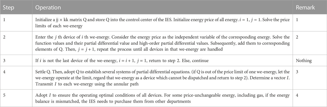
TABLE 5. APDA.

Remark 1: Here, $\text{jj}$ denotes the price-changeable energy type. In this article, $\text{jj}$ is 2 because the power and heat price can be changed; however, the gas price cannot be changed. We should add some initialization values into $\mathrm{Q}$ and store $\mathrm{Q}$ into the control center. The reason behind that will be introduced later. Moreover, $\text{kk}$ indicates the order limit. In this study, $\text{kk}$ is 2. The order limit analysis will be introduced in the proceeding sections.

Remark 2: The rows of $\mathrm{Q}$ represent devices with each single price-changeable energy. The model in this article comprises two rows, which correspond to power and heat. The first column of $\mathrm{Q}$ contains the function values of $f_w\left(x\right)$ corresponding to energy. The second column of $\mathrm{Q}$ contains the first-order partial differential of the corresponding independent variable in the first column. The APDA will add corresponding energy and corresponding partial into the corresponding place. It is worth mentioning that two or more different values can be added into one place. We can use the model in this study as an example.

${\mathrm{Q}}^{+}=\left[\begin{array}{cc}A& A_1\\ B& B_1\end{array}\right],(15)$

$A={\displaystyle \sum }_{j\subset \left\{\mathrm{1,2,8,11,4,7}\right\}}{x}_{i,j}^1,(16)$

$A_1={\displaystyle \sum }_{j\subset \left\{\mathrm{1,2,8,11,4,7}\right\}}\frac{\partial \left(C\right)}{\partial \left(x_{i,j}^1\right)},(17)$

$B={\displaystyle \sum }_{j\subset \left\{\mathrm{3,9,12,4,7}\right\}}{x}_{i,j}^2,(18)$

$B_2={\displaystyle \sum }_{j\subset \left\{\mathrm{3.9,12,4,7}\right\}}\frac{\partial \left(C\right)}{\partial \left(x_{i,j}^2\right)},(19)$

where $Q^{-}$ is the $\mathrm{Q}$ before step 2.

Remark 3: First, the $Q$ in step 4 should be settled. There are two $Q$ s in the control center: first, we store an initialization $Q$ in the control center in step 1, which we named $Q^1$; second, we use the algorithm to compute a $Q$ and transmit it to the control center, which we named $Q^2$.

$\mathrm{Q}={\mathrm{Q}}^1-{\mathrm{Q}}^2.(20)$

Subsequently, we establish $jj$ functions. These functions are $f_{ww}\left(x\right),\left(ww\subset \left\{\mathrm{1,2,3},\dots ,jj\right\}\right)$. We establish a system of partial differential equations as

$\left\{\frac{{\partial }^{kk}\left(f_{ww}\right)}{\partial {\left(x\right)}^{kk}}=Q\left(ww,kk+1\right)\left|kk\ge 0\right.\right\}.(21)$

Accordingly, all $f_{ww}$ can be solved.

Subsequently, we should use these $f_{ww}$ to ensure energy balance. Because all function values of each $f_{ww}$ denote the total energy in the IES, if all $f_{ww}$ values are 0, the energy balance is reached. However, that is not the optimization condition because the energy conversion is not considered. There are three circumstances that could be considered in this article

Circumstance 1: One price-changeable energy a changes to another price-changeable energy b.

Circumstance 2: One price-changeable energy a changes to one price-unchangeable energy b.

Circumstance 3: One price-unchangeable energy b changes to one price-changeable energy a.

In circumstance 1, we should solve these functions.

$x_a=x_b,(22)$

${f_{ww}}^a=-{f_{ww}}^b\ge 0,(23)$

where $x$ indicates the independent variable of $f_{ww}$; $f_{ww}^a$ and $f_{ww}^b$ are the $f_{ww}$ of energy a and b, respectively.

In circumstance 2, we should solve the following functions.

$x_a=prb,(24)$

${f_{ww}}^a\ge 0,(25)$

where $\text{prb}$ indicates the energy price of b.

In circumstance 3, we are required to solve the following functions.

$x_a=prb,(26)$

${f_{ww}}^a\le 0.(27)$

Other $f_{ww}$ without energy transformation are all 0.

Accordingly, we can solve these functions to work out all $x$ of each $f_{ww}$ and all conversion energies. We adopt each $x$ of the corresponding energy as the energy prices and divide the energy conversion value to all energy transformation devices. We add all energy prices and divided the conversion energy value into $I$.

Remark 4: The optimization operating condition of each energy devices can be solved as

$\max W={\displaystyle \sum }_{ww=1}^m{x}_{i,j,t_k}^{ww}prww-C,(\mathrm{28a})$

where $C$ represents the cost function and $\text{prww}$ indicates the energy price of the $ww$-th energy. Furthermore, all conditions of conversion devices are in $I$.

Remarkably, the reason for placing a random initialized value into $Q$ in the first step is to protect privacy. In the APDA, each device can only know the sum of the data; hence, they cannot know the data of each device. However, the second device can know the data of the first device because the total data are the data of the first device. Accordingly, we place an initialized value into $Q$ in the first step to protect the data of the first device.

3.4 Demonstration of the proposed algorithm

First, we should prove some propositions.

Proposition 1: The cost price of energy is the differential of its cost function.

First, because all cost functions are convex, the energy cost price is dynamic. The average energy cost price between $x$ and $x_0$ can be given as

$\mathit{pr}=\frac{C\left(x\right)-C\left(x_0\right)}{x-x_0}(\mathrm{28b})$

If for all positive values $\epsilon$, $\left|x_0-x\right|<\epsilon$, we can draw a conclusion that

$\mathit{pr}=\frac{C\left(x\right)-C\left(x_0\right)}{x-x_0}=C^{\prime }\left(x\right)(29)$

Accordingly, the cost price on $x$ is the differential of $C\left(x\right)$.

Proposition 2: If there is only one type of energy in the IES, the best operating condition of each device is that all first-order differentials are the same.

We assume another operating condition in the IES. Some devices named condition 2 with less cost based on the condition that all first-order differentials are the same, which is named condition 1. The energy balances are satisfied in conditions 1 and 2.

There are some devices in condition 2 with more energy than that in condition 1. To ensure energy balance, there are also some devices in condition 3 with less energy than that in condition 1. Accordingly, the devices with more energy consume more cost, and vice-versa. Conditions 2 and 3 collectively constitute another operating condition of the IES.

For conditions 1 and 2, we assume $x$ is energy in condition 1, $x_n$ is energy in condition 2. $n\subseteq \left\{\mathrm{1,2},\dots ,\mathrm{m}\right\}$, and $\mathrm{m}$ indicates all devices with more energy in condition 2. From the Lagrange mean value theorem, we can draw a conclusion that

$C^{\prime }\left(x\right)\le \frac{C\left(x_n\right)-C\left(x\right)}{x_n-x}=\underset{\delta \subset \left(x,x_n\right)}{C^{\prime }}\left(\delta \right)\le C^{\prime }\left(x_n\right).(30)$

The cost between condition 1 and condition 2 is

$C\mathit{\text{more}}={\displaystyle \sum }_{n\subseteq \left\{\mathrm{1,2},\dots ,\mathrm{m}\right\}}C\left(x_n\right)-C\left(x\right)={\displaystyle \sum }_{n\subseteq \left\{\mathrm{1,2},\dots ,\mathrm{m}\right\}}{\underset{\delta \subset \left(x,x_n\right)}{C}}^{\prime }\left(\delta \right)\left(x_n-x\right).(31)$

We name all the energy as $xx$ and the smallest ${\underset{\delta \subset \left(x,x_n\right)}{C}}^{\prime }\left(\delta \right)$ in $n\subseteq \left\{\mathrm{1,2},\dots ,\mathrm{m}\right\}$ is $C_{\nabla }$. Thus, we obtain

$C\mathit{\text{more}}={\displaystyle \sum }_{n\subseteq \left\{\mathrm{1,2},\dots ,\mathrm{m}\right\}}{\underset{\delta \subset \left(x,x_n\right)}{C}}^{\prime }\left(\delta \right)\left(x_n-x\right)\ge C_{\nabla }{\displaystyle \sum }_{n\subseteq \left\{\mathrm{1,2},\dots ,\mathrm{m}\right\}}\left(x_n-x\right)=C_{\nabla }xx>C^{\prime }\left(x\right)xx.(32)$

For conditions 1 and 3, we assume $x$ is energy in condition 1, $x_k$ is energy in condition 3. $k\subseteq \left\{\mathrm{1,2},\dots ,\text{mm}\right\}$, and $\text{mm}$ indicates all devices with more energy in condition 3. From the Lagrange mean value theorem, we can draw a conclusion that

$C^{\prime }\left(x_k\right)\le \frac{C\left(x\right)-C\left(x_k\right)}{x-x_k}={\underset{\delta \subset \left(x,x_n\right)}{C}}^{\prime }\left(\varphi \right)\le C^{\prime }\left(x\right).(33)$

The lesser cost between condition 1 and condition 2 is given as

$\mathit{Cless}={\displaystyle \sum }_{k\subseteq \left\{\mathrm{1,2},\dots ,\mathrm{m}\mathrm{m}\right\}}C\left(x\right)-C\left(x_k\right)={\displaystyle \sum }_{k\subseteq \left\{\mathrm{1,2},\dots ,\mathrm{m}\mathrm{m}\right\}}{\underset{\delta \subset \left(x_k,x\right)}{C}}^{\prime }\left(\varphi \right)\left(x-x_k\right)(34)$

We name all less energy as $xxx$, and the largest ${\underset{\delta \subset \left(x_k,x\right)}{C}}^{\prime }\left(\varphi \right)$ in $k\subseteq \left\{\mathrm{1,2},\dots ,mm\right\}$ is $C_{\nabla \nabla }$. Thus, we obtain

$\mathit{Cless}={\displaystyle \sum }_{k\subseteq \left\{\mathrm{1,2},\dots ,mm\right\}}{\underset{\varphi \subset \left(x_k,x\right)}{C}}^{\prime }\left(\varphi \right)\left(x-x_k\right)\le C_{\nabla \nabla }{\displaystyle \sum }_{k\subseteq \left\{\mathrm{1,2},\dots ,mm\right\}}\left(x-x_k\right)=C_{\nabla \nabla }xxx<C^{\prime }\left(x\right)xxx.(35)$

To ensure energy balance, $xxx=xx$, which yields

$\mathit{Cless}<C^{\prime }\left(x\right)xxx=C^{\prime }\left(x\right)xx<C\mathit{\text{more}}.(36)$

Thus, the best operating condition for all devices require that all first-order differentials be the same. Proposition 2 stands correct.

Similarly, if the price of energy a is the same as that of energy b, the energy transformation is the optimal condition. Accordingly, the optimization is proved.

4 Simulation results

The simulation results of this study are divided into five parts: 1) the running results of the APDA, 2) the running results of the existing iterative algorithm and subsequent comparison with the APDA (including the benchmark functions test for the APDA and the existing iterative algorithm), 3) the plug-and-play performance test of the APDA, 4) emergency power dispatch of the APDA, and 5) scalability of the APDA. We chose the iterative algorithm presented in Chang et al. (2021) as a comparative benchmark. To attain a more convincing comparison, the simulation platform, all device types, arguments and quantities, and loads of all energies are the same as those depicted in the literature (Chang et al., 2021) (only gas-based CHP is deleted because gas is very expensive currently; therefore, it is inadvisable to adopt gas to produce other energies. To make the comparison more convincing, gas-based CHP is not only deleted from the simulation results of the APDA but also from the simulation results of the existing iterative algorithm presented in (Chang et al., 2021)). The data are provided in the Supplementary Material. It is worth noting that the data of the APDA and traditional algorithms are kept the same for comparison. The integrated energy system model of the APDA and that of the comparative algorithm are shown in Figure 2. More details and data are available in literature (Chang et al., 2021) and will not be repeated here. It should be noted that the cyber information communication path for the APDA is a simple annular path. However, the energy transmission path is not circular. The cyber information communication path only transmits information but not energy because if energy is transmitted in a simple circle, the energy transmission cost will be very high. After running the APDA, the balance of all energies was achieved. Then, how to transmit corresponding energies to corresponding we-energies will be an easy elementary mathematical problem that does not require any algorithms. Therefore, this study does not discuss the energy transmission path. Figure 2 shows an energy transmission black box that replaces the energy transmission topology. In each we-energy, there is one control center, one wind generator, one solar generator, one solar heat device, one coal-based CHP, one electric boiler, one equivalent gas producer (only in we-energy 1), one power storage device, one heat store device, one gas store device, one power to gas device, and one electric boiler. All data are in the Supplementary Material.

FIGURE 2

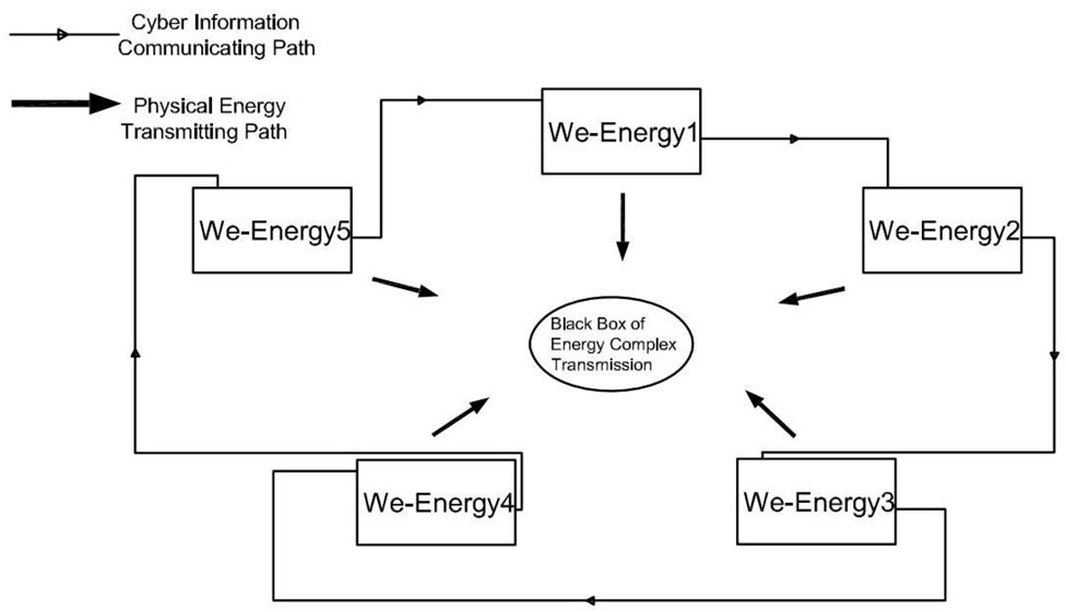
FIGURE 2. IES model.

The simulation result of the APDA is shown in Figure 3 (because the APDA does not require iterations, there are no convergence procedures for the APDA. It converges in one iteration.). The abscissas 1–11 in Figure 3 represent the power rate of the wind generator, power rate of the solar generator, heat rate of the solar heat devices, gas rate of the equivalent gas producer (if there is no equivalent gas producer, that value is zero), power rate of the coal-based CHP, heat rate of the coal-based CHP, power rate of the power storage device, heat rate of the heat store device, gas rate of the gas store device, power rate of the electric boiler, and power rate of the power to gas device. The power, heat, and gas prices were 11.2198 cents, 8.4393 cents, and 7.6237 cents, respectively, per$kwh$. Additionally, the APDA requires only one iteration; thus, the algorithm is exceedingly fast and communication and computation burden is exceedingly low. Furthermore, the energy supply demand mismatches of power, heat, and gas are all 0. In addition, there were no parameters that were difficult to adjust. For the existing iterative algorithm (setting the price adjustment factor to ${10}^{-8}$), the convergence procedure with iterations of power–heat–gas prices and power–heat–gas supply demand mismatch are shown in Figures 4–9, respectively (the Zeno coefficient is defined in Tan and Li, (2022). Because the Zeno coefficient is not related to the APDA and is only connected to a traditional algorithm for contrast experiments, it is not detailed here. The detail about the algorithm for contrast experiments is in the Supplementary Material). The power, heat, and gas prices were 11.1620 cents, 8.3847 cents, and 7.6237 cents, respectively, per $kwh$. Additionally, this algorithm requires 50 iterations, which not only reduces the speed of the algorithm considerably but also significantly increases the communication and computational burden. Furthermore, the energy supply-demand mismatches of power, heat, and gas are 2,714 $kwh$ less, 3,262 $kwh$ less, and 0, respectively. In addition, the algorithm is highly sensitive to suitable factors. If we adjust the price adjustment factor to ${10}^{-6}$, the power–heat–gas supply-demand mismatch will vibrate, as shown in Figure 10, Figure 11, and Figure 12, and never reach the energy balance.

FIGURE 3

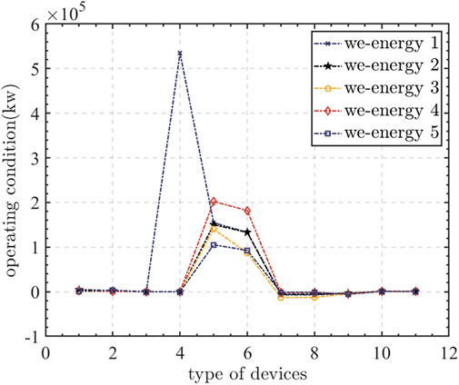
FIGURE 3. Simulation results of the APDA.

FIGURE 4

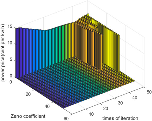
FIGURE 4. Convergence procedure of power price.

FIGURE 5

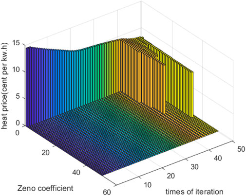
FIGURE 5. Convergence procedure of heat price.

FIGURE 6

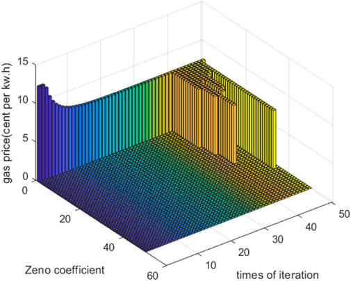
FIGURE 6. Convergence procedure of gas price.

FIGURE 7

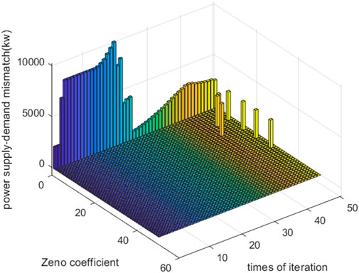
FIGURE 7. Convergence procedure of power supply-demand mismatch.

FIGURE 8

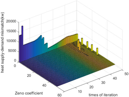
FIGURE 8. Convergence procedure of heat supply-demand mismatch.

FIGURE 9

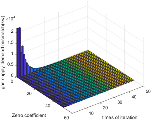
FIGURE 9. Convergence procedure of gas supply-demand mismatch.

FIGURE 10

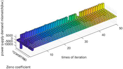
FIGURE 10. Power mismatch with larger factor.

FIGURE 11

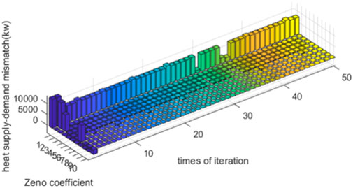
FIGURE 11. Heat mismatch with larger factor.

FIGURE 12

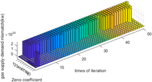
FIGURE 12. Gas mismatch with larger factor.

In summary, both the APDA and traditional algorithm can unify all prices of one energy in each device. According to the theoretical demonstration presented in Section 3.4, if all prices of one energy are unified, optimization can be achieved. Therefore, both the APDA and traditional algorithm can be optimized. However, the APDA can strictly realize the astringency of all energy mismatches to 0, but the traditional algorithm can only converge the power–heat–gas mismatch to 2,714 $kwh$ less, 3,262 $kwh$ less, and 0. Therefore, the APDA has better astringency than the traditional algorithms. In addition, because the APDA only requires one iteration, whereas the traditional algorithm requires 50 iterations, the communication and computational burden in the APDA is much less than that in the traditional algorithm. Accordingly, the APDA is much faster than the traditional algorithm; therefore, it can avoid the time delay better than traditional algorithms. Finally, the APDA is independent of suitable factors, whereas traditional algorithms rely heavily on them.

To test the plug-and-play performance of the APDA, we removed the last we-energy in the simulation platform. The simulation results are shown in Figure 13. The abscissas 1–11 in Figure 13 represent the same meaning as those presented in Figure 3. Figure 13 shows that the APDA can operate normally without we-energy; therefore, the plug-and-play performance of the APDA is reliable.

FIGURE 13

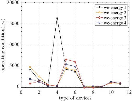
FIGURE 13. Plug-and-play performance.

It should be noted that the variations in power loads and fluctuations experienced by power devices are usually in the order of several seconds, while the heat and gas load variations in the IES are usually hourly. Thus, based on the hourly dispatch of all energies, an emergency strategy for power-only devices (including power in CHP) is required for emergency power scheduling. If power scheduling is required, the APDA operates with power-only devices. We increased the 50,000 $kw$ power ratio to test emergency power scheduling. The simulation result is presented in Figure 14. The abscissas 1–11 in Figure 14 represent the same values as those depicted in Figure 3. From Figure 14, we can conclude that the emergency power scheduling of the APDA is reliable.

FIGURE 14

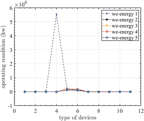
FIGURE 14. Emergency power scheduling.

As for testing the scalability of the IES, we have already established a large-scale system by adding the we-energy number from 5 to 15 to test the scalability of the proposed method. All data are in the Supplementary Material. The simulation result is in Figure 15. The abscissas 1–10 in Figure 15 represent the power rate of the wind generator, power rate of the solar generator, heat rate of the solar heat devices, power rate of the coal-based CHP, heat rate of the coal-based CHP, power rate of the power storage device, heat rate of the heat store device, gas rate of the gas store device, power rate of the electric boiler, and power rate of the power to gas device. The gas rate of the equivalent gas producer is 11,221,474 $kwh$. We do not put it into the figure because it is too large. However, the equivalent gas producer is not limited by the network limit because of the reason we have already introduced in Section 2. From Figure 15, we can conclude that the emergency power scheduling of the APDA is reliable.

FIGURE 15

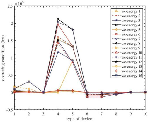
FIGURE 15. Scalability performance.

5 Conclusion

In this study, an algorithm without iterations called the APDA was introduced for use in future IES applications. By comparing the currently proposed and traditional algorithms, we determine that the APDA only requires one communication and computation iteration, whereas the traditional algorithm requires 50 iterations. In addition, the APDA can strictly realize the astringency of all energy mismatches to 0. However, the traditional algorithm can only reduce the power–heat–gas mismatch to 2,714 $kwh$ less, 3,262 $kwh$ less, and 0. In addition, the APDA is independent of suitable factors, whereas traditional algorithms rely heavily on them. However, the APDA requires synchronous communication and large-scale communication simultaneously. Some changeable IES applications are unfit because they require frequent dispatches. In addition, the APDA can only handle convex optimization; accordingly, an IES with non-convex devices is unsuitable for it. Therefore, asynchronous communication without iteration and non-convex optimization in an IES needs to be further studied.

Data availability statement

The original contributions presented in the study are included in the article/Supplementary Material; further inquiries can be directed to the corresponding author.

Author contributions

XL has corrected the format. Other study is carried out by JT.

Conflict of interest

The authors declare that the research was conducted in the absence of any commercial or financial relationships that could be construed as a potential conflict of interest.

Publisher’s note

All claims expressed in this article are solely those of the authors and do not necessarily represent those of their affiliated organizations, or those of the publisher, the editors, and the reviewers. Any product that may be evaluated in this article, or claim that may be made by its manufacturer, is not guaranteed or endorsed by the publisher.

Supplementary material

The Supplementary Material for this article can be found online at: https://www.frontiersin.org/articles/10.3389/fenrg.2022.1078938/full#supplementary-material

References

Abessi, A., and Jadid, S. (2021). Internal combustion engine as a new source for enhancing distribution system resilience. J. Mod. Power Syst. Clean Energy 9 (5), 1130–1136. doi:10.35833/mpce.2019.000246

CrossRef Full Text | Google Scholar

Binetti, G., Davoudi, A., Lewis, F. L., Naso, D., and Turchiano, B. (2014). Distributed consensus-based economic dispatch with transmission losses. IEEE Trans. Power Syst. 29 (4), 1711–1720. doi:10.1109/tpwrs.2014.2299436

CrossRef Full Text | Google Scholar

Chang, X., Xu, Y., and Sun, H. (2021). Online distributed neurodynamic optimization for energy management of renewable energy grids. Int. J. Electr. Power & Energy Syst. 130, 106996. doi:10.1016/j.ijepes.2021.106996

CrossRef Full Text | Google Scholar

Chen, G., Lewis, F. L., Feng, E. N., and Song, Y. (2015). Distributed optimal active power control of multiple generation systems. IEEE Trans. Ind. Electron. 62 (11), 7079–7090. doi:10.1109/tie.2015.2431631

CrossRef Full Text | Google Scholar

Chen, Y., Yao, Y., Lin, Y., and Yang, X. (2022). Dynamic state estimation for integrated electricity-gas systems based on extended Kalman filter[J]. CSEE J. Power Energy Syst. 8 (1), 293–303.

Google Scholar

Feng, J., Liu, L., Pei, Q., and Li, K. (2022). Min-max cost optimization for efficient hierarchical federated learning in wireless edge networks. IEEE Trans. Parallel Distrib. Syst. 33 (11), 1–2700. doi:10.1109/tpds.2021.3131654

CrossRef Full Text | Google Scholar

Feng, J., Zhang, W., Pei, Q., Wu, J., and Lin, X. (2022). Heterogeneous computation and resource allocation for wireless powered federated edge learning systems. IEEE Trans. Commun. 70 (5), 3220–3233. doi:10.1109/tcomm.2022.3163439

CrossRef Full Text | Google Scholar

Guo, L., Yang, B., Ye, J., Chen, H., Li, F., Song, W., et al. (2021). Systematic assessment of cyber-physical security of energy management system for connected and automated electric vehicles. IEEE Trans. Ind. Inf. 17 (5), 3335–3347. doi:10.1109/tii.2020.3011821

CrossRef Full Text | Google Scholar

Guo, Y., Tong, L., Wu, W., Zhang, B., and Sun, H. (2017). Coordinated multi-area economic dispatch via critical region projection. IEEE Trans. Power Syst. 32 (5), 3736–3746. doi:10.1109/tpwrs.2017.2655442

CrossRef Full Text | Google Scholar

He, X., Ai, Q., Qiu, R. C., Huang, W., Piao, L., and Liu, H. (2017). A big data architecture design for smart grids based on random matrix theory. IEEE Trans. Smart Grid 8 (2), 674–686.

Google Scholar

Hu, X., Zhang, H., Ma, D., Wang, R., and Tu, P. (2022). Small leak location for intelligent pipeline system via action-dependent heuristic dynamic programming. IEEE Trans. Ind. Electron. 69 (11), 11723–11732. doi:10.1109/tie.2021.3127016

CrossRef Full Text | Google Scholar

Hua, H., Hao, C., Qin, Y., and Cao, J. (2018). A class of control strategies for energy internet considering system robustness and operation cost optimization. Energies 11 (6), 1593. doi:10.3390/en11061593

CrossRef Full Text | Google Scholar

Huang, M., Wei, Z., and Lin, Y. (2022). Forecasting-aided state estimation based on deep learning for hybrid AC/DC distribution systems[J]. Applied Energy, 306, 118119, doi:10.1016/j.apenergy.2021.118119

CrossRef Full Text | Google Scholar

Kirli, D., Couraud, B., Robu, V., Salgado-Bravo, M., Norbu, S., Andoni, M., et al. (2022). Smart contracts in energy systems: A systematic review of fundamental approaches and implementations. Renew. Sustain. Energy Rev. 158, 112013. doi:10.1016/j.rser.2021.112013

CrossRef Full Text | Google Scholar

Lai, X., Zhong, H., Xia, Q., and Kang, C. (2017). Decentralized intraday generation scheduling for multiarea power systems via dynamic multiplier-based Lagrangian relaxation. IEEE Trans. Power Syst. 32 (1), 454–463. doi:10.1109/tpwrs.2016.2544863

CrossRef Full Text | Google Scholar

Liu, G., Sun, Q., Liang, H., and Liu, Z. (2021). Antagonistic interactions-based adaptive event-triggered bipartite consensus quantized control for stochastic multiagent systems. IEEE Syst. J., 1–12. doi:10.1109/JSYST.2021.3116035

CrossRef Full Text | Google Scholar

Liu, G., Sun, Q., Wang, R., and Hu, X. (2022). Nonzero-sum game-based voltage recovery consensus optimal control for nonlinear microgrids system. IEEE Trans. Neural Netw. Learn. Syst., 1–13. doi:10.1109/TNNLS.2022.3151650

PubMed Abstract | CrossRef Full Text | Google Scholar

Liu, L., Zhao, M., Yu, M., Jan, M. A., Lan, D., and Taherkordi, A. (2022). Mobility-aware multi-hop task offloading for autonomous driving in vehicular edge computing and networks. IEEE Trans. Intell. Transp. Syst., 1–14. doi:10.1109/TITS.2022.3142566

CrossRef Full Text | Google Scholar

Ma, D., Cao, X., Sun, C., Wang, R., Sun, Q., Xie, X., et al. (2022). Dual-predictive control with adaptive error correction strategy for AC microgrids. IEEE Trans. Power Deliv. 37 (3), 1930–1940. doi:10.1109/tpwrd.2021.3101198

CrossRef Full Text | Google Scholar

Ma, D., Hu, X., Zhang, H., Sun, Q., and Xie, X. (2021). A hierarchical event detection method based on spectral theory of multidimensional matrix for power system. IEEE Trans. Syst. Man. Cybern. Syst. 51 (4), 2173–2186. doi:10.1109/tsmc.2019.2931316

CrossRef Full Text | Google Scholar

Mao, S., Liu, L., Zhang, N., Dong, M., Zhao, J., Wu, J., et al. (2022). Reconfigurable intelligent surface-assisted secure mobile edge computing networks. IEEE Trans. Veh. Technol. 71 (6), 6647–6660. doi:10.1109/TVT.2022.3162044

CrossRef Full Text | Google Scholar

Mishra, D. K., Ghadi, M. J., Li, L., Zhang, J., and Hossain, M. (2022). Active distribution system resilience quantification and enhancement through multi-microgrid and mobile energy storage. Appl. Energy 311, 118665. doi:10.1016/j.apenergy.2022.118665

CrossRef Full Text | Google Scholar

Tan, J., and Li, H. (2022). Annular directed distributed algorithm for energy internet[J]. International Transactions on Electrical Energy Systems, (1), 7717605, doi:10.1155/2022/7717605

CrossRef Full Text | Google Scholar

Tan, Jiaming. (2022). Energy management without iteration—a regional dispatch event-triggered algorithm for energy internet. Front. Energy Res. 10 (2022), 908199. doi:10.3389/fenrg.2022.908199

CrossRef Full Text | Google Scholar

Tan, X., Cao, M., Cao, J., Xu, W., and Luo, Y. (2021). Event-triggered synchronization of multiagent systems with partial input saturation. IEEE Trans. Control Netw. Syst. 8 (3), 1406–1416. doi:10.1109/tcns.2021.3065667

CrossRef Full Text | Google Scholar

Wang, R., Sun, Q., Sun, C., Zhang, H., Gui, Y., and Wang, P. (2021). Vehicle-vehicle energy interaction converter of electric vehicles: A disturbance observer based sliding mode control algorithm. IEEE Trans. Veh. Technol. 70 (10), 9910–9921. doi:10.1109/tvt.2021.3105433

CrossRef Full Text | Google Scholar

Wei, W., Gu, H., Deng, W., Xiao, Z., and Ren, X. (2022). ABL-TC: A lightweight design for network traffic classification empowered by deep learning. Neurocomputing 489, 333–344. doi:10.1016/j.neucom.2022.03.007

CrossRef Full Text | Google Scholar

Wei, W., Yang, R., Gu, H., Zhao, W., Chen, C., and Wan, S. (2021). Multi-objective optimization for resource allocation in vehicular cloud computing networks. IEEE Trans. Intell. Transp. Syst., 1–10. doi:10.1109/TITS.2021.3091321

CrossRef Full Text | Google Scholar

Xing, H., Mou, Y., Fu, M., and Lin, Z. (2015). Distributed bisection method for economic power dispatch in smart grid. IEEE Trans. Power Syst. 30 (6), 3024–3035. doi:10.1109/tpwrs.2014.2376935

CrossRef Full Text | Google Scholar

Xu, B., Ge, Y., Liu, Y., Qi, J., Sun, Y., et al. (2019). Optimization of an intelligent community hybrid energy system with robustness consideration. IEEE Access, 7, PP 58780–58790. doi:10.1109/ACCESS.2019.2914696

CrossRef Full Text | Google Scholar

Yang, L., Sun, Q., Zhang, N., and Liu, Z. (2020). Optimal energy operation strategy for we-energy of energy internet based on hybrid reinforcement learning with human-in-the-loop. IEEE Trans. Syst. Man. Cybern. Syst. 52 (1), 32–42. doi:10.1109/tsmc.2020.3035406

CrossRef Full Text | Google Scholar

Yang, Y., Tan, Z., Yang, H., Ruan, G., et al. (2022). Short-term electricity price forecasting based on graph convolution network and attention mechanism[J]. IET Renewable Power Generation, 16(12):2481-2492. doi:10.1049/rpg2.12413

CrossRef Full Text | Google Scholar

Zhang, H., Li, Y., Gao, D. W., and Zhou, J. (2017). Distributed optimal energy management for energy internet. IEEE Trans. Ind. Inf. 13 (6), 3081–3097. doi:10.1109/tii.2017.2714199

CrossRef Full Text | Google Scholar

Zhao, F., Litvinov, E., and Zheng, T. (2014). A marginal equivalent decomposition method and its application to multi-area optimal power flow problems. IEEE Trans. Power Syst. 29 (1), 53–61. doi:10.1109/tpwrs.2013.2281775

CrossRef Full Text | Google Scholar

Zhou, G., Tian, Q., and Wang, L. (2021). Soft-switching high gain three-port converter based on coupled inductor for renewable energy system applications. IEEE Trans. Ind. Electron. 69 (99), 1521–1536. doi:10.1109/tie.2021.3060614

CrossRef Full Text | Google Scholar

Zhou, J., Xu, Y., Sun, H., Li, Y., and Chow, M. (2020). Distributed power management for networked AC/DC microgrids with unbalanced microgrids. IEEE Trans. Ind. Inf. 16 (3), 1655–1667. doi:10.1109/tii.2019.2925133

CrossRef Full Text | Google Scholar

Zhou, J., Xu, Y., Sun, H., Wang, L., and Chow, M. -Y. (2020). Distributed event-triggered $H_\infty$ consensus based current sharing control of DC microgrids considering uncertainties. IEEE Trans. Ind. Inf. 16 (12), 7413–7425. doi:10.1109/TII.2019.2961151

CrossRef Full Text | Google Scholar