Disturbance auto-encoder generation model: Few-shot learning method for IGBT open-circuit fault diagnosis in three-phase converters

With the rapid development of converters in a variety of industrial fields, the fault diagnosis of power switching devices has become an important factor in ensuring the safe and reliable operation of related systems. In recent years, machine learning has performed well in many fault diagnosis tasks. The success of these advanced methods depends on sufficient marked samples for each fault type. However, in most industrial applications, it is expensive and difficult to collect fault samples, and the fault diagnosis model trained under the limited samples cannot meet the requirements of fault diagnosis accuracy. In order to solve this problem, this study proposes a few-shot learning method based on fault sample generation to realize the open-circuit fault diagnosis of IGBT in a three-phase PWM converter. This method is the deformation of the auto-encoder called the disturbance auto-encoder generation model. By designing the model structure and training algorithm constraints, the encoder learns the nonlinear transferable disturbance from the normal operating sample pairs. Then, the disturbance is applied to the decoder to synthesize new fault samples to realize the training of the fault diagnosis model with limited samples. The biggest advantage of this method is that it can achieve 95.90% fault diagnosis accuracy by only collecting the samples in the normal operating conditions of the target system. Finally, the feasibility and advantages of the proposed method are verified by comparative experiments.

1 Introduction

The three-phase PWM converters are composed of power switches (such as insulated gate bipolar transistor IGBT) and related control systems, which have the advantages of high efficiency, high power density, and low harmonic content. These characteristics make the three-phase PWM converters widely used in motor drive, wind power generation, photovoltaic (PV) power generation, and other industrial scenarios. However, due to equipment aging, overload, or accidents, power switches are prone to failure during operation. According to recent reports, power switches are the most vulnerable components in converters, especially in these high-power applications (Liang et al., 2022). The faults of power switches occur in the form of short or open circuits. Short circuit faults will lead to over current or over temperature, usually using the hardware circuit for protection and then converting to open-circuit faults. Conversely, the implicit fault characteristics of open-circuit faults are often insufficient to trigger hardware protection and cannot be discovered in time, resulting in secondary faults. Therefore, the demands and interests in the development of IGBT open-circuit fault diagnosis are increasing, which provides the necessary information for maintenance and fault-tolerant control to make the system more reliable (Malik et al., 2022).

In general, fault diagnosis methods can be divided into model-based, signal-based, and knowledge-based methods (Gao et al., 2015a). As classic methods, the model-based methods are used to establish the model of industrial or system process, which comes from physical principles or system identification techniques (Zhuo et al., 2020; Wassinger et al., 2018; Yu et al., 2017; Poon et al., 2016; Xie and Ge, 2018; Hwang and Huh, 2015), such as observer methods (Yu et al., 2017; Wassinger et al., 2018; Zhuo et al., 2020), state estimation techniques (Poon et al., 2016; Xie and Ge, 2018), and parity equations (Hwang and Huh, 2015). By calculating and monitoring the residuals between model generation outputs and measured outputs, anomalies and faults are detected and located. However, model-based methods rely heavily on accurate mathematical models, which may result in model uncertainty and difficulty in identifying parameters. For difficult-to-model systems, signal-based methods (Abari et al., 2017; Zhou et al., 2018a; Zhou et al., 2018b; Huang et al., 2021) (Abari et al., 2017; Zhou et al., 2018a; Zhou et al., 2018b; Huang et al., 2021) are widely used to detect the characteristic distortion of sampled signals. Signal-based methods mainly use signal processing techniques and rely on prior knowledge, which may bring a heavy computational burden and excessive diagnosis time.

In recent years, with the significant progress of machine learning technology, knowledge-based methods have attracted considerable research attention (Gao et al., 2015b; Wang et al., 2015; Cai et al., 2016a; Cai et al., 2016b; Cai et al., 2016c; Moosavi et al., 2016; Cherif and Bendiabdellah, 2018; Huang et al., 2018; Ding et al., 2019; Xia et al., 2019; Ye et al., 2019; Gou et al., 2020) (Gao et al., 2015b; Wang et al., 2015; Cai et al., 2016a; Cai et al., 2016b; Cai et al., 2016c; Moosavi et al., 2016; Cherif and Bendiabdellah, 2018; Huang et al., 2018; Ding et al., 2019; Xia et al., 2019; Ye et al., 2019; Gou et al., 2020). The principle is to extract the mapping relationship between measurement data and fault labels. In offline training, the fault database is used to train the machine learning-based classification model. In online applications, the classification model generates fault diagnosis results based on input signals (i.e., sampling current and voltage). Unlike model-based and signal-based methods, knowledge-based methods are independent of the system model and signal processing, making them more robust and generalizable in changing systems (Gao et al., 2015b). The classical classification model is generally divided into two steps: feature extraction and fault classification. Feature extraction methods mainly include fast Fourier transform (FFT) (Cai et al., 2016a; Cai et al., 2016b; Moosavi et al., 2016; Xia et al., 2019; Gou et al., 2020) (Cai et al., 2016a; Cai et al., 2016b; Moosavi et al., 2016; Xia et al., 2019; Gou et al., 2020), discrete wavelet transform (DWT) (Cherif and Bendiabdellah, 2018; Ye et al., 2019), principal ingredient analysis (PCA) (Wang et al., 2015), and linear discriminant analysis (Ding et al., 2019). Fault classification methods include support vector machine (SVM) (Huang et al., 2018), Bayesian network (Cai et al., 2016a; Cai et al., 2016b) (Cai et al., 2016a), and neural network (Wang et al., 2015; Moosavi et al., 2016; Cherif and Bendiabdellah, 2018; Xia et al., 2019; Ye et al., 2019; Gou et al., 2020).

Although these machine learning-based classifiers can perform nonlinear learning, traditional feature extraction methods are inductive biased, leading to the loss of valuable information. Recently, deep learning models with fault feature extraction capabilities have greatly improved fault diagnosis capabilities. Si et al. (2022) used a deep LSTM network with attention cooperation to extract discriminative features from the original data. Compared with other methods, it has better diagnostic results under various conditions. Yuan et al. (2022) used 1-DCNN to extract features from the original data, and 100% accuracy of fault diagnosis was realized perfectly in the experiment of the IGBT open-circuit fault diagnosis for NPC inverters. However, in order to train a reliable classification model, a large amount of fault data are required that can fully reflect the real operating conditions of the target system, which is particularly important for deep learning models. However, in most cases, the fault experiment of the target system is expensive, and its safety risk is unacceptable, such as wind power generation and the traction system (Cai et al., 2016b). For most knowledge-based methods, the classification model is trained from the source database of a particular system in a simulation or ideal experiment. Various uncertain disturbances occur between the source and target systems, such as load characteristics, sensors, and grid disturbances, resulting in model and feature mismatches, which cause unacceptable fault misdiagnosis rates (Xia and Xu, 2021).

In recent years, few-shot learning has provided a promising research direction to solve the above problems (Wang et al., 2020). The purpose of few-shot learning is to train the models under the condition of limited marked data or different tasks similar to the target task (Lai et al., 2020). Generally, it can be divided into sample generation, model, and algorithm. Compared with the model and algorithm, the data generation methods only need a simple classification model, so it is favored by the high real-time fault diagnosis task (Li et al., 2020; Liu et al., 2021; Pei et al., 2021; Li et al., 2020; Liu et al., 2021; Pei et al., 2021; Li et al., 2020; Liu et al., 2021; Pei et al., 2021). Li et al. (2020) proposed five simple signal deformation techniques to generate samples that train deep learning models. Under the condition of limited samples, good fault diagnosis results of rotating machinery were obtained. In addition, Liu et al. (2021) proposed a sample generation model named variational auto-encoding generative adversarial networks (VAGAN) with deep regret analysis to improve the fault diagnosis ability of the rolling bearing fault. Pei et al. (2021) proposed an enhanced few-shot Wasserstein auto-encoder (EFWAN) to generate samples for reliable fault diagnosis of rolling bearing with limited data. In summary, few-shot learning methods have achieved great success in image recognition, natural language processing, and fault diagnosis, among others (Parnami and Lee, 2022; Snell et al., 2017). However, to the best knowledge of the authors, there are almost no reports on the few-shot learning for converter fault diagnosis. In the converter fault diagnosis, it is usually required to make a fault diagnosis every cycle (0.001–0.025 s). The high real-time requirements and the complexity of the algorithms bring great challenges to the limited computing resources. In addition, in order to ensure the reliable operation of the converter, a false diagnosis is unacceptable.

In order to solve the above problems, a few-shot learning method based on sample generation is proposed in this study. In the case of limited databases, we can synthesize enough samples for each category to train the classifier in a standard supervised way without increasing the computational burden on the classifier. Firstly, in order to improve the performance of sample generation, the key factors are revealed in the error decomposition of few-shot learning (Section 2.2). Then, based on the key factors, a disturbance auto-encoder generation model is proposed through model design and training algorithm constraints. The proposed disturbance auto-encoder generation model trains an encoder and a decoder from the source database (simulation database). In the generation phase, the encoder extracts the disturbance from the same class sample pairs, whereas the decoder uses disturbance and source samples to reconstruct the fault samples for the target system. Therefore, the generated samples can better fit the sample distribution of the target system. The main contributions of this paper are as follows:

1) An disturbance auto-encoder generation model is proposed in this study, which can synthesize the fault sample data of the target system only by collecting the data of the target system under normal operating conditions. The proposed generation model effectively solves the problem of collecting IGBT open-circuit fault data of the converter.

2) The classifier trained by the synthesized samples has high fault diagnosis accuracy without increasing the computational burden on the online classification.

3) In the comparative experiments of two databases, the effectiveness and superiority of the disturbance auto-encoder generation model are verified.

The rest of this study is organized as follows: Section 2 briefly introduces the topology of the three-phase converter system and defines the IGBT open-circuit fault labels. The few-shot learning error analysis shows that the performance of the generation model depends on whether the generation samples are identically distributed with the target system. Section 3 describes in detail the proposed disturbance auto-encoder generation model. Section 4 gives the experimental results and discussion. Finally, a general conclusion is given.

2 System and critical problem descriptions

2.1 System description

A widely used three-phase PWM converter topology is shown in Figure 1, which consists of six IGBT modules (T₁—T₆) and their auxiliary control units. i_a, i_b, and i_c are the three-phase output currents of the converter. This study discusses the most common single and double IGBT open-circuit faults in practical applications. A total of 22 fault labels, including normal conditions, are shown in Table 1, and each label represents a specific fault type. The proposed fault diagnosis method uses the machine learning method as the fault classifier. The inputs are i_a, i_b, and i_c, and the outputs are the fault labels. The fault location is realized in Table 1.

FIGURE 1

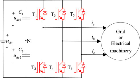
FIGURE 1. Three-phase PWM converter topology.

TABLE 1

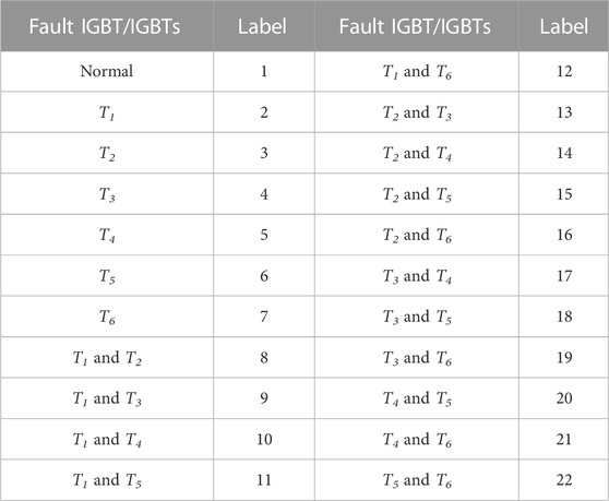
TABLE 1. Labels of IGBT open-circuit fault.

2.2 Error decomposition of few-shot learning

In any classification tasks of machine learning, perfect classification cannot be obtained, and there are usually classification errors. This section illustrates the core issues of few-shot learning through error decomposition based on supervised machine learning (Bottou and Bousquet, 2008; Bottou et al., 20182018). The analysis shows that the performance of the sample generation model depends on whether the generated samples are identically distributed with the target system samples.

Generalization error: Given a classification task, p(x, y) represents the joint probability distribution of the feature vector x and the classification label y, and there is an optimal assumption $\overline{h}$ that minimizes the generalization error e, where a and b are arbitrary variables and I(a,b) is a function:

$\mathit{e}\left(\overline{\mathit{h}}\right)=\int \mathit{I}\left(\overline{\mathit{h}}\left({\mathit{x}}_{\mathit{i}}\right),{\mathit{y}}_{\mathit{i}}\right)\mathit{d}\mathit{p}\left({\mathit{x}}_{\mathit{i}},{\mathit{y}}_{\mathit{i}}\right),$

$\mathit{I}\left(\mathit{a},\mathit{b}\right)=\left\{\begin{array}{cc}\mathbf{1},& \mathit{a}\ne \mathit{b}\\ \mathbf{0},& \mathit{a}=\mathit{b}\end{array}\right..(1)$

Model error: For a given hypothesis space H, when the training sets of N_l samples are sufficient to estimate p(x,y), there exists a function $h^{*}\in$ H that minimizes the model error e_m:

$e_m=\frac{\mathbf{1}}{N_l}{{\displaystyle \sum }}_{i=\mathbf{1}}^{N_l}I\left(h^{*}\left(x_i\right),y_i\right)p\left(x_i,y_i\right).(2)$

Empirical error: When the datasets D_train of N_s samples are small, p(x, y) is unknown. Exist $h_s\in$ H minimizing the empirical error e_s as fellows:

$e_s=\frac{\mathbf{1}}{N_s}{\sum }_{i=\mathbf{1}}^{N_s}I\left(h_s\left(x_i\right),y_i\right).(3)$

Therefore, the error of few-shot learning can be decomposed into

$\mathit{{\rm E}}\left(\mathit{e}\left({\mathit{h}}_{\mathit{s}}\right)-\mathit{e}\left(\overline{\mathit{h}}\right)\right)=\underset{{\mathit{e}}_{\mathit{m}\mathit{g}}\left(\mathit{H}\right)}{\underset{}{\mathit{{\rm E}}\left(\mathit{e}\left({\mathit{h}}^{*}\right)-\mathit{e}\left(\overline{\mathit{h}}\right)\right)}}+\underset{{\mathit{e}}_{\mathit{s}\mathit{m}}\left(\mathit{H},{\mathit{N}}_{\mathit{s}}\right)}{\underset{}{\mathit{{\rm E}}\left(\mathit{e}\left({\mathit{h}}_{\mathit{s}}\right)-\mathit{e}\left({\mathit{h}}^{*}\right)\right)}}.(4)$

E represents expectation. As shown in Eq. 4, the error of few-shot learning is affected by the sample N_s in the D_train and hypothesis space H. In other words, reducing the error of few-shot learning can be attempted from the perspective of enhancing data, providing a D_train sufficient to estimate $p\left(\mathrm{x},y\right)$. In addition, from Eqs 2–4, in order to reduce $e_{sm}\left(H,N_s\right)$, the key is to keep identical distribution p(x,y) between generated samples and target samples.

3 Proposed disturbance auto-encoder generation model

3.1 Main ideas

The premise of machine learning fault diagnosis methods is that there are enough fault samples. However, the collection of target system fault samples is usually expensive and difficult due to the risk of fault experiments (Liang et al., 2022). On the contrary, it is easier to construct a fault database through the source system (simulation, ideal experiment, and existing samples of similar systems) (Cai et al., 2016b). However, the models trained by the source system are often not well applied to the target system. The main reason is that the target system has a variety of uncertain disturbances, such as load disturbance, sensor noise, and grid disturbance (Xia and Xu, 2021). It is worth noting that the above disturbance will not change with the occurrence of the open-circuit fault of IGBT. Therefore, it has the transferable ability from normal to fault conditions. In addition, if sufficient normal operation samples are used to extract the above disturbance, the disturbance implicitly contains the information of the $p\left(x,y\right)$.

In order to accurately extract the above disturbance, our method is inspired by Hariharan and Girshick (2017) and Eli Schwartz (2017), where a relative offset between a pair of the same class conveys valid deformation information, and the same offset is applied to other examples to synthesize new samples. In our technique, we do not limit disturbance to relative offset. In principle, a model can be constructed to learn the nonlinear transferable disturbance of the target system under different operating conditions.

The proposed model comprises encoder E and decoder D, which is the deformation of the auto-encoder. The schematic diagram of the proposed method is shown in Figure 2. The encoder E extracts the nonlinear transferable disturbance Z from the normal operating current data of the source and target domain. The decoder D uses the fault samples of the source domain and Z to generate the fault samples of the target domain.

FIGURE 2

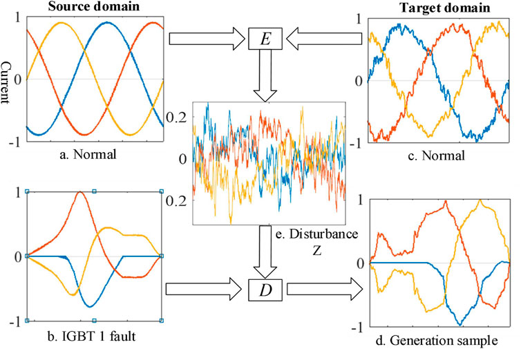
FIGURE 2. Schematic diagram of the proposed method.

Specifically, the standard auto-encoder (Kingma and Welling, 2013) reconstructs the signal X_s by minimizing $‖X_s-\overline{X_s}‖$, where $\overline{X_s}=D\left(E\left(X_s\right)\right)$ represents the signal reconstructed by the encoder. Usually, the dimension of $Z_s=E\left(X_s\right)$ is much smaller than X_s, representing the minimum dimension of feature vector required to reconstruct X_s, indicating that the encoder can extract features. We use structural design and training method constraints to enable E to extract the disturbance Z_s from the same class sample pairs and let Z_s represent the necessary information required to synthesize X_sn from X_sp to ensure the fault characteristics of the generation samples. X_sp and X_sn represent the same class samples.

3.2 Model structure and training method

Model structure: The structure of the proposed disturbance auto-encoder generation model is shown in Figure 3, which is divided into two stages: training and generation. In the training phase, the inputs are the same class of fault sample pairs (X_sn, X_sp) from the two source databases (s and p), and Z_s is obtained by the encoder E. Then, Z_s and X_sn are used as the inputs of the decoder D to obtain the synthetic sample of X_sp. Finally, the forward propagation of the training phase is expressed as

$\overline{X_{sp}}=D\left({\mathrm{\Theta }}_D,E\left({\mathrm{\Theta }}_E,X_{sn},X_{sp}\right),X_{sn}\right).(5)$

FIGURE 3

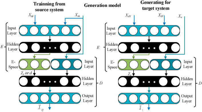
FIGURE 3. Structure of the proposed disturbance auto-encoder generation model.

${\mathrm{\Theta }}_D$ and ${\mathrm{\Theta }}_E$ are parameters that need to be solved for the auto-encoder. In order to ensure the complexity of Z_s, E, and D are fit by the similar n-layer 1-dimension convolution neural network (1-DCNN). The details of 1-DCNN can be found in Yuan et al. (2022).

In the generation phase, sufficient samples are collected from the normal operational target system to implicitly include p(x, y). The sample pairs (X_sN, X_tN), formed by the normal operational target and source system, are used as the inputs of the encoder E to obtain Z_t. Then, Z_t and X_s are used as inputs to decoder D to get the generation samples. X_tN represents the sample mean of the normal operational target and source system, and X_s represents the sample mean of a certain fault class in the source system. Finally, the forward propagation of the generation phase is expressed as

$\overline{X_t}=D\left({\mathrm{\Theta }}_D,E\left({\mathrm{\Theta }}_E,X_{sN},X_{tN}\right),X_s\right).(6)$

Model training: In order to solve the parameters ${\mathrm{\Theta }}_D$ and ${\mathrm{\Theta }}_E$ and make Z_s represent the nonlinear transferable disturbance, we constrain Z_s by Gaussian distribution injection. This is based on the fact that the output disturbance is caused by a variety of random factors. Therefore, Z_s can be approximated to Gaussian noise by the central limit theorem. To this end, the training of the model is conducted in two stages. In the first stage, Z_s is replaced by Gaussian distribution noise $d\sim \mathrm{N}\left(0,\sigma \right)$. Then, d and X_sp are used as input to train decoder D with the following training objective:

$D\left(\overline{{\mathrm{\Theta }}_D},d,X_{sp},\right)\sim \overline{{\mathrm{\Theta }}_D}=\underset{{\mathrm{\Theta }}_D}{argmin}{‖D\left({\mathrm{\Theta }}_D,d,X_{sn}\right)-X_{sp}‖}^{\mathbf{2}}.(7)$

It can be proved that the training results of the above models are as follows (see Appendix A for details):

$D\left(\overline{{\mathrm{\Theta }}_D},d,X_{sn,i}\right)={\rm E}\left(\overline{{X_{sp}}_{,i}}\right).(8)$

Among them, $X_{sn,i}$ represents the i-class fault samples in X_sn and $\overline{{X_{sp}}_{,i}}$ represents the sample mean of the i-class fault in X_sp. The above training makes the decoder D encoded by d, and its generation samples retain the fault feature as the i-class fault sample mean ${\rm E}\left(\overline{{X_{sp}}_{,i}}\right)$.

In the second stage, training the encoder E and fine-tuning the decoder D, X_sn and X_sp are used as inputs. The generation model has the following training objectives:

$\begin{array}{c}D\left(\widehat{{\mathrm{\Theta }}_D},E\left(\overline{{\mathrm{\Theta }}_E},X_{sp},X_{sn}\right),X_{sp}\right)\sim \widehat{{\mathrm{\Theta }}_D},\overline{{\mathrm{\Theta }}_E}\\ \underset{{\mathrm{\Theta }}_D,{\mathrm{\Theta }}_E}{=argmin}{‖D\left({\mathrm{\Theta }}_D,E\left({\mathrm{\Theta }}_E,X_{sp}\right)\right)-X_{sn}‖}^{\mathbf{2}}...\\ +{\lambda }_D{‖{\mathrm{\Theta }}_D-\overline{{\mathrm{\Theta }}_D}‖}^{\mathbf{2}}\end{array}(9)$

The first term is to minimize the synthesis error, and the second term is the decoder fine-tuning term. Under the premise of ensuring the synthesis sample error, the closer ${\mathrm{\Theta }}_D$ is to $\overline{{\mathrm{\Theta }}_D}$, the closer Z_s is to d, so that Z_s can represent the nonlinearity transferable disturbance.

The training process is shown in Algorithm 1.

3.3 Implementation details

In all experiments, the sample feature vector X is handled from the outputs i_a, i_b, i_c of the converter by period normalization, frequency normalization, and amplitude normalization. Period normalization: Separate current by one period, and the first feature in the feature vector corresponds to the forward crossing zero of ia. Frequency normalization: The number of sample points of a periodic signal is fixed, and 224 sample points are used for the feature vector in this study. Amplitude normalization: Each sample point is divided by a maximum value in a period. E and D are based on the same structure as the 1-DCNN, with model parameters shown in Table 2.

TABLE 2

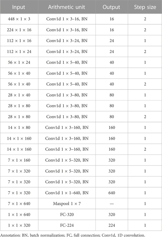
TABLE 2. Model parameters of 1-DCNN for decoder and encoder.

These models are trained with the Adam optimizer, and the learning rate was set to 10−⁵. When the number of training sample pairs is 2,000 × 22, the sample generation model training takes about 20 cycles to achieve convergence. Each epoch runs for approximately 184 s on the Nvidia Tesla K40m GPU (88K training samples, batch size 128). It takes approximately 16.8 s to generate data per 1,024 samples.

4 Experimental verification and discussion

4.1 Database and experimental settings

This study constructs two kinds of source-target databases to verify the performance of the proposed generation model. Database 1 is from the PV grid-connected converter, and database 2 is from the three-phase permanent magnet synchronous motor drive converter. The source databases are obtained by simulation (MATLAB-Simulink) with the consistent experiment parameters of the target system. The target databases are obtained by fault experiment, considering the DC voltage ripple, power, load, sensor bias, sensor noise, and other disturbance factors. All databases are handled from the outputs i_a, i_b, i_c of the converters by period normalization, frequency normalization, and amplitude normalization. The data acquisition process is set as shown in Tables 3, 4. Because the fault experiment of the target system is difficult, the number of target fault databases is relatively small.

TABLE 3

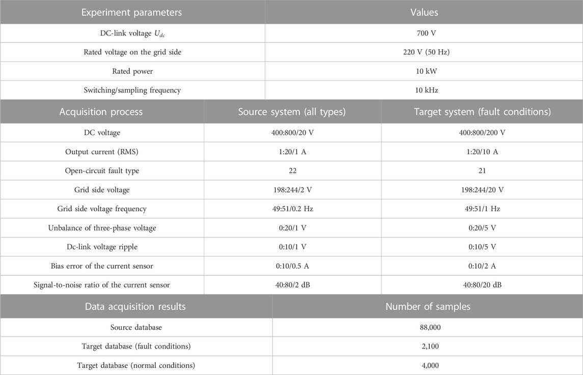
TABLE 3. Database 1 acquisition process.

TABLE 4

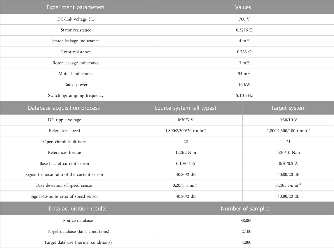
TABLE 4. Database 2 acquisition process.

In order to train the proposed disturbance auto-encoder generation model, we group source database 1 and source database 2 according to the operating conditions (from large to small) to obtain 88,000 training sample pairs of (X_sn, X_sp). During sample generation, 4,000 sets of normal operating sample pairs (X_sN, X_tN) of the source and target systems are formed as inputs according to operating conditions (from large to small). Then, samples are generated based on few-shot test requirements.

In the comparative analysis, the proposed method is compared with two types of sample generation models (Liu et al., 2021; Pei et al., 2021) by constructing few-shot test episodes. In each test episode of N-way-k-shot fault diagnosis tasks, we randomly select N invisible fault categories and extract k random samples from each category of the target dataset. During sample generation, the trained disturbance auto-encoder generation model is used to synthesize 1,024 samples for each category. The inputs of the disturbance auto-encoder generation model are from the normal condition sample pairs (X_sN, X_tN) and the k fault condition sample pairs (X_sF, X_tF), respectively. In particular, when k = 0 is a zero-shot-learning task, only (X_sN, X_tN) is used to generate samples.

After the sample generation is completed, train the popular classifiers, including the Bayesian network, support vector machine (SVM), and 1-DCNN. Finally, GAN-test calculates the classification accuracy of M test samples of N categories from the target database.

4.2 The quality analysis of generation samples

In order to evaluate the performance of the proposed disturbance auto-encoder generation model, the generation samples are verified in two datasets. Firstly, the time domain waveforms of the generation samples are qualitatively compared. Secondly, two commonly used evaluation indicators for the sample generation model, MMD and KL divergence, are used for quantitative evaluation (Liu et al., 2021).

In qualitative analysis, the time domain waveform of source, target, and generation samples are compared under the same operating conditions. Meanwhile, the difference degree of samples is evaluated by the average variance. The IGBT T₁ open-circuit faults are shown in Figure 4A; Figure 5A, and the T₃ and T₅ faults are shown in Figure 4B; Figure 5B. The figures show high similarity between the generation and target sample under the same operating condition. In contrast, the similarity is low between the source and the target sample.

FIGURE 4

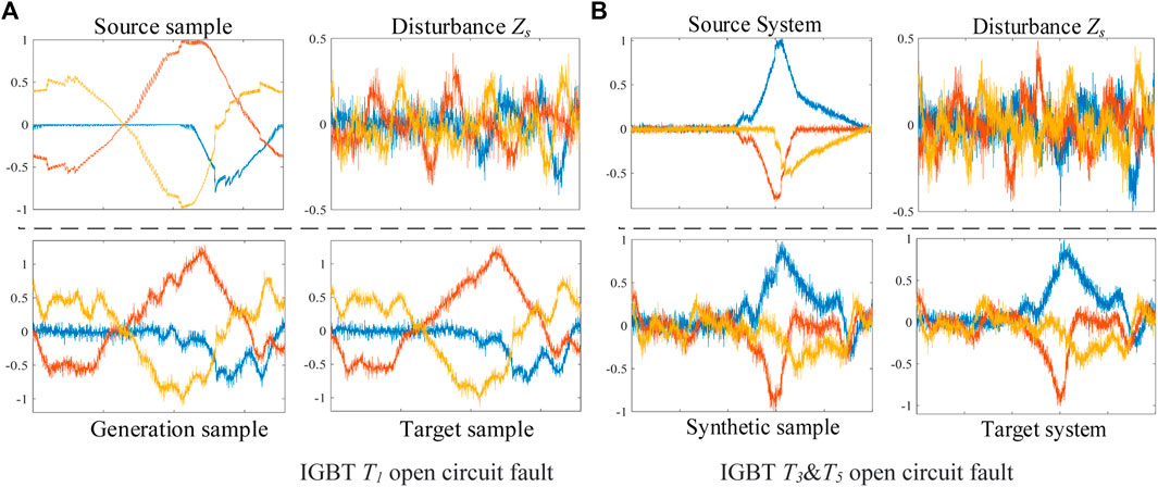
FIGURE 4. Comparison of generation samples in database 1: (A) IGBT T₁ open-circuit fault, (B) IGBT T₃ and T₅ open-circuit fault.

FIGURE 5

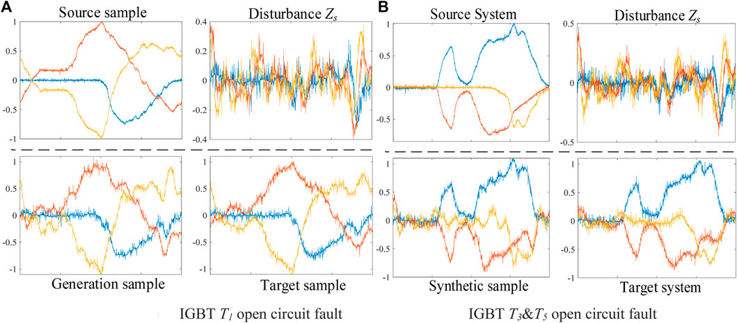
FIGURE 5. Comparison of generation samples in database 2: (A) IGBT T₁ open-circuit fault, (B) IGBT T₃ and T₅ open-circuit fault.

In addition, the extracted disturbance exhibits Gaussian distribution characteristics. Comparing Figures 4A, B and Figures 5A, B, the disturbances extracted from different faults are similar, proving its fault transferable ability.

The average variance is calculated in Table 5, indicating that the difference between the generation-target data is much smaller than the difference between the source-target data. Therefore, the sample generation model proposed in this study has excellent performance. In addition, the small difference degree of disturbance further proves its fault transferable ability.

TABLE 5

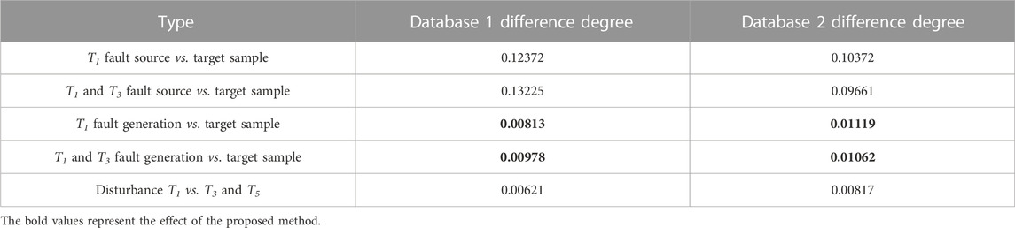
TABLE 5. Difference degree of generation under the same operating conditions.

In order to quantitatively evaluate the performance of generation samples, MMD and KL divergences are introduced. MMD maps each sample into Hilbert space and calculates its average value, which is used to measure the similarity between the distribution of the generation and the target database. The smaller the value, the closer the two distributions are. KL divergence is an asymmetric measure of the difference between the distributions of two datasets and is used to express the distance between any two distributions. The comparison evaluation results of different sample generation methods are shown in Table 6. All methods produce the same number of generation samples for each type of fault.

TABLE 6

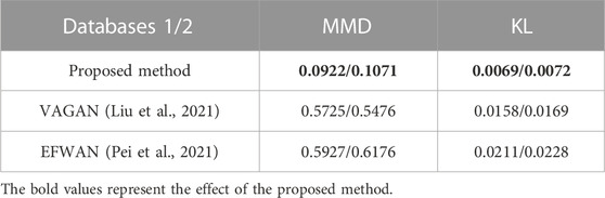
TABLE 6. Evaluation results of quantitative indexes of generated samples.

Table 6 shows that the KL divergence and MMD values of the proposed method are the smallest among the three sample generation methods, indicating that the generation sample distribution by the proposed method is the closest to the target sample, so the sample quality is the best (Vinyals et al., 2016) because the proposed method considers the feature distribution of the target system.

4.3 Few-shot fault diagnosis comparison test

In order to further verify the few-shot diagnosis effect of the proposed generation model, a comparative experiment with sample generation methods (Liu et al., 2021; Pei et al., 2021) is performed in N-way-K-shot tasks. All methods have the same number of generation samples. After sample generation, the average performance of fault diagnosis accuracy on 10 such experiments is evaluated in several classification algorithms. The comparison results of fault diagnosis accuracy are shown in Figure 6.

FIGURE 6

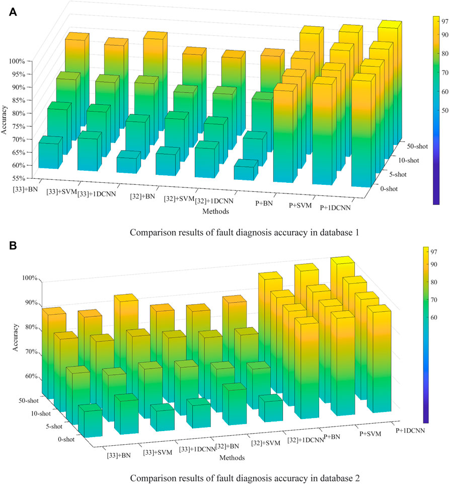
FIGURE 6. (A) Comparison results of fault diagnosis accuracy in database 1. (B) Comparison results of fault diagnosis accuracy in database 2.

Figure 6 shows that the proposed method is superior to those of Liu et al. (2021) and Pei et al. (2021) in all few-shot tasks. Among them, the proposed method + 1DCNN has the best performance, with a fault diagnosis accuracy of 95.90% in a zero-shot task and with fault diagnosis accuracy of 99.87% in a 50-shot task. In addition, compared with Hariharan and Girshick (2017) and Eli Schwartz (2017), with the increase of N (N-shot), the fault diagnosis accuracy of the proposed method does not improve significantly because this method can extract the feature distribution from normal operating conditions, whereas Hariharan and Girshick (2017) and Eli Schwartz (2017) need to extract the feature distribution of fault samples from N. Another phenomenon is that when the sample quality is higher, the fault accuracy of 1-DCNN is higher, which indicates that the deep learning model has superior feature extraction ability, but data dependence is the most serious. Although the SVM and Bayesian network are simple, the performance exceeds 1-DCNN when the sample quality is poor, which reflects that both sample quality and classifier performance are important factors in determining fault diagnosis accuracy of IGBT open-circuit fault. Finally, a comparison of Figures 6A, B shows that the performance is consistent in different databases, which proves the universality of the above rules. Detailed data are shown in Table 7.

TABLE 7

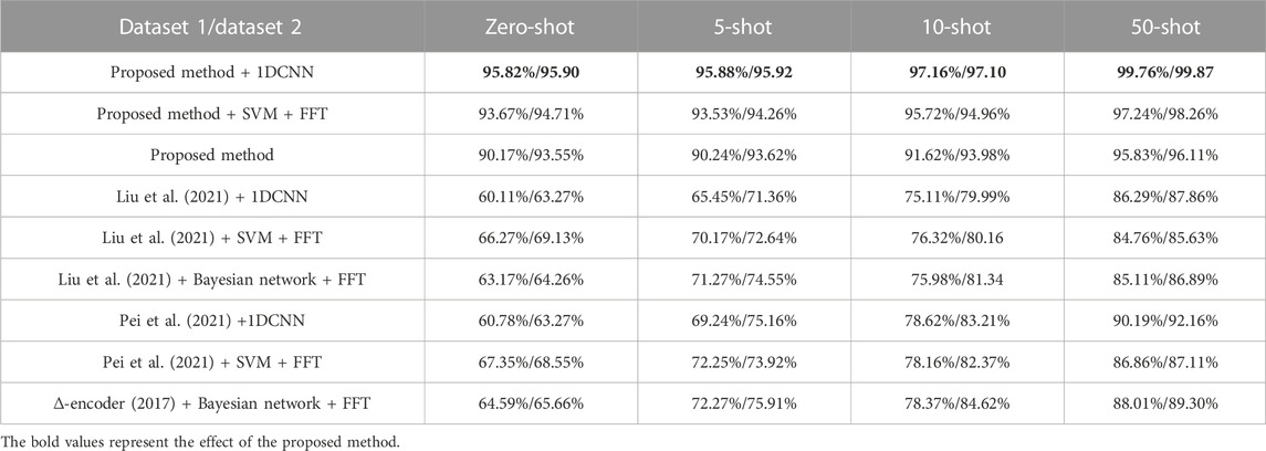
TABLE 7. Diagnosis accuracy evaluation results.

In order to reduce the risk and cost of fault collection in the target system, the research objective of this study is to collect only the normal operation samples in the target system to form a reliable fault diagnosis model. Therefore, it is necessary to visually evaluate the performance of the proposed method + 1-DCNN in the 0-way-10-shot task. The confusion matrix and S-TNE, which is a dimensionality reduction method, are adopted.

The confusion matrix in Figure 7 shows that in the 0-shot task, the proposed method does not diagnose the fault sample as a normal sample, nor does it diagnose the normal sample as a fault sample. Therefore, there is no risk of false diagnosis, and it has reliable engineering application value. The dimensionality reduction results of S-TNE of the last layer feature of 1-DCNN are shown in Figure 8. Different types of samples are separated from each other, indicating that the proposed method has better fault diagnosis capabilities, and the generation samples are close to the target samples, further proving that the proposed generation model can better fit the fault sample distribution of the target system.

FIGURE 7

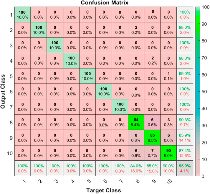
FIGURE 7. Confusion matrix of + 1-DCNN in the 0-shot task.

FIGURE 8

FIGURE 8. S-TNE results of + 1-DCNN in the 0-shot task.

4.4 Online fault diagnosis experiment

In order to verify the application effect of the proposed method in practical engineering, an online fault diagnosis experiment is performed on the three-phase PV grid-connected converter. The experiment system, as shown in Figure 9, consists of a three-phase grid-connected converter and a fault diagnosis system. The three-phase grid-connected converter is composed of PV analog power supply (CHROMA 62024), grid analog power supply (CHROMA 61702), main power circuit (IGBT and filter), and a control system. The controller is DSP28377S, with a sampling frequency of 20 kHz and a control frequency of 10 kHz. The output current data in the controller are transmitted to the fault diagnosis system through DMA after downsampling processing. The fault diagnosis system comprises FPGA (Speedster7t) and its auxiliary unit, which is used to realize fast parallel computing of 1D-CNN. When the fault is detected, the fault diagnosis result is sent to the control unit to realize the rapid protection and control of the PV grid-connected system.

FIGURE 9

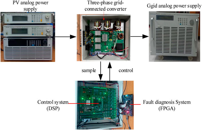
FIGURE 9. Experimental platform.

In this study, the T₁ open-circuit fault and T₁ and T₃ open-circuit faults are taken as examples to illustrate the effectiveness of the proposed method. Once the open-circuit fault is detected, the controller will immediately shut down all IGBTs to protect the system and then start the fault-tolerant control units according to the fault diagnosis result. The experimental results are shown in Figure 10.

FIGURE 10

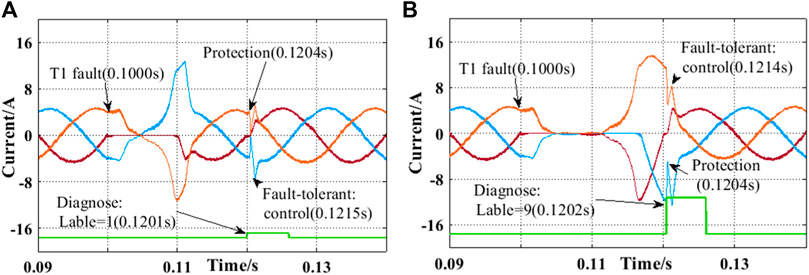
FIGURE 10. Fault diagnosis results, (A) T₁ open-circuit faults, (B) T₁ and T₃ open-circuit faults.

In Figure 10A, IGBT T₁ has an open-circuit fault at 0.1 s, whereas the fault diagnosis system locates the fault (label = 1) at 0.1201 s and issues protection instructions to the controller. The controller shuts down the system at 0.1204, so the current drops rapidly to avoid secondary failures. After that, the standby IGBT is started at 0.1215 s to realize fault-tolerant control and resume operation. The same experimental effect for T₁ and T₃ open-circuit faults appears similarly in Figure 10B. The proposed method only takes about 0.0215 from failure occurrence to recovery control. Therefore, it meets the real-time requirement of converter fault diagnosis. It is proved that the few-shot learning method proposed in this study will not increase the computational burden of the fault classifier.

In more detail, Figures 10A, B show that using the proposed method, the IGBT open-circuit fault can be identified in around one current cycle (20.1–20.2 m). The online calculation time is minor, around 0.1–.2 m. Once IGBT open-circuit failure occurs, the proposed method can quickly turn off the system within about 0.4 m to avoid more serious secondary accidents. Then, the fault tolerant control system is quickly started according to the fault diagnosis results (approximately 1.4–1.5 m). The above experiments demonstrate the engineering feasibility of the proposed method. When the IGBT open-circuit fault occurs, the proposed method can ensure the continuous operation of the system and greatly improve its reliability. In addition, the fault diagnosis results can guide the maintenance and greatly reduce its cost.

5 Conclusion

In order to solve the problem of data collection in the IGBT open-circuit fault diagnosis of a three-phase PWN converter, achieving reliable data-driven fault diagnosis model training under limited samples, this study presents a few-shot learning method based on data generation. The method, which is called the disturbance auto-encoder generation model, consists of an encoder and a decoder. Through model design and training algorithm constraints, the decoder extracts nonlinear transferable disturbance from the normal operating conditions of the target system, and the decoder synthesizes the target system samples by combining the disturbance and source samples. As the extracted disturbance considers the feature distribution of the target system and has fault feature transferable capability, the generation samples can well fit the feature distribution of the target system. Using the generated samples to train the 1-DCNN fault model, it does not need to collect the target system fault samples and achieves 95.90% fault diagnosis accuracy in 0-shot and 99.87% fault diagnosis accuracy in the 50-shot task, which is a new breakthrough in the research field of few-shot learning-based fault diagnosis method. Finally, the online fault diagnosis performance of the method is verified in PV grid-connected converter experimental prototype, showing that the proposed method has excellent real-time and fault-tolerant control ability. In future work, a more complex engineering environment to verify the performance of the method is worth trying.

Data availability statement

The raw data supporting the conclusion of this article will be made available by the authors, without undue reservation.

Author contributions

Conceptualization, FW; methodology, GQ; software, FW; formal analysis, LZ; resources, KC; writing—original draft preparation, FW; writing—review and editing, LW; validation JY and JG; supervision, GQ; project administration, FW; funding acquisition, KC. All authors read and agreed to the published version of the manuscript.

Funding

This research was partly funded by the Fundamental Research Funds for the Central Universities under Grant no. ZYGX2020ZB004, the Sichuan Science and Technology Project under Grant no. 2019ZDZX0045, and the second batch of industry-university cooperation collaborative education projects of the Ministry of Education in 2021 (202102371056).

Conflict of interest

The authors declare that the research was conducted in the absence of any commercial or financial relationships that could be construed as a potential conflict of interest.

Publisher’s note

All claims expressed in this article are solely those of the authors and do not necessarily represent those of their affiliated organizations or those of the publisher, the editors, and the reviewers. Any product that may be evaluated in this article, or claim that may be made by its manufacturer, is not guaranteed or endorsed by the publisher.

References

Abari, I., Lahouar, A., Hamouda, M., Slama, J. B. H., and Al-Haddad, K. (2017). Fault detection methods for three-level NPC inverter based on DC-bus electromagnetic signatures. IEEE Trans. Industrial Electron. 65 (7), 5224–5236. doi:10.1109/tie.2017.2777378

CrossRef Full Text | Google Scholar

Bottou, L., Curtis, F. E., and Nocedal, J. (2018). Optimization methods for large-scale machine learning. SIAM Rev. 60, 2223–2311. doi:10.1137/16m1080173

CrossRef Full Text | Google Scholar

Bottou, L., and Bousquet, O. (2008). “The tradeoffs of large scale learning,” in Advances in neural information processing systems (Massachusetts, MA, USA: MIT Press), 161–168.

Google Scholar

Cai, B., Liu, H., and Xie, M. (2016). A real-time fault diagnosis methodology of complex systems using object-oriented Bayesian networks. Mech. Syst. Signal Process. 80, 31–44. doi:10.1016/j.ymssp.2016.04.019

CrossRef Full Text | Google Scholar

Cai, B., Liu, Y., and Xie, M. (2016). A dynamic-bayesian-network-based fault diagnosis methodology considering transient and intermittent faults. IEEE Trans. Automation Sci. Eng. 14 (1), 276–285. doi:10.1109/tase.2016.2574875

CrossRef Full Text | Google Scholar

Cai, B., Zhao, Y., Liu, H., and Xie, M. (2016). A data-driven fault diagnosis methodology in three-phase inverters for PMSM drive systems. IEEE Trans. Power Electron. 32 (7), 5590–5600. doi:10.1109/tpel.2016.2608842

CrossRef Full Text | Google Scholar

Cherif, B. D. E., and Bendiabdellah, A. (2018). Detection of two-level inverter open-circuit fault using a combined DWT-NN approach. J. Control Sci. Eng. 2018, 1–11. doi:10.1155/2018/1976836

CrossRef Full Text | Google Scholar

Ding, S., Li, X., Hang, J., and Wang, Y. (2019). Application of hybrid dimensionality reduction for fault diagnosis of three-phase inverter in PMSM drive system. Electr. Eng. 101 (3), 813–827. doi:10.1007/s00202-019-00823-8

CrossRef Full Text | Google Scholar

Gao, Z., Cecati, C., and Ding, S. X. (2015). A survey of fault diagnosis and faultfault-tolerant techniques—Part I: Fault diagnosis with model-based and signal-based approaches. IEEE Trans. Industrial Electron. 62 (6), 3757–3767. doi:10.1109/tie.2015.2417501

CrossRef Full Text | Google Scholar

Gao, Z., Cecati, C., and Ding, S. X. (2015). A survey of fault diagnosis and faulttolerant techniques—part II: Fault diagnosis with knowledge-based and hybrid/active approaches. IEEE Trans. Ind. Electron. 62 (6), 1–3774. doi:10.1109/tie.2015.2419013

CrossRef Full Text | Google Scholar

Gou, B., Xu, Y., Xia, Y., Deng, Q., and Ge, X. (2020). An online data-driven method for simultaneous diagnosis of IGBT and current sensor fault of three-phase PWM inverter in induction motor drives. IEEE Trans. Power Electron. 35 (12), 13281–13294. doi:10.1109/tpel.2020.2994351

CrossRef Full Text | Google Scholar

Hariharan, B., and Girshick, R. “Low-shot visual recognition by shrinking and hallucinating features,” in Proceedings of the IEEE international conference on computer vision, Venice, Italy, 2017, 3018–3027.

Google Scholar

Huang, W., Du, J., Hua, W., Lu, W., Bi, K., Zhu, Y., et al. (2021). Current-based open-circuit fault diagnosis for PMSM drives with model predictive control. IEEE Trans. Power Electron. 36 (9), 10695–10704. doi:10.1109/tpel.2021.3061448

CrossRef Full Text | Google Scholar

Huang, Z., Wang, Z., and Zhang, H. (2018). A diagnosis algorithm for multiple open-circuited faults of microgrid inverters based on main fault component analysis. IEEE Trans. Energy Convers. 33 (3), 925–937. doi:10.1109/tec.2018.2822481

CrossRef Full Text | Google Scholar

Hwang, W., and Huh, K. (2015). Fault detection and estimation for electromechanical brake systems using parity space approach. J. Dyn. Syst. Meas. Control 137 (1). doi:10.1115/1.4028184

CrossRef Full Text | Google Scholar

Kingma, D. P., and Welling, M. (2013). Auto-encoding variational bayes. https://arxiv.org/abs/1312.6114.

Google Scholar

Lai, N., Kan, M., Han, C., Song, X., and Shan, S. (2020). Learning to learn adaptive classifier–predictor for few-shot learning. IEEE Trans. neural Netw. Learn. Syst. 32 (8), 3458–3470. doi:10.1109/tnnls.2020.3011526

PubMed Abstract | CrossRef Full Text | Google Scholar

Li, X., Zhang, W., Ding, Q., and Sun, J. Q. (2020). Intelligent rotating machinery fault diagnosis based on deep learning using data augmentation. J. Intelligent Manuf. 31 (2), 433–452. doi:10.1007/s10845-018-1456-1

CrossRef Full Text | Google Scholar

Liang, J., Zhang, K., Al-Durra, A., Muyeen, S., and Zhou, D. (2022). A state-of-the-art review on wind power converter fault diagnosis. Energy Rep. 8, 5341–5369. doi:10.1016/j.egyr.2022.03.178

CrossRef Full Text | Google Scholar

Liu, S., Jiang, H., Wu, Z., and Li, X. (2021). Rolling bearing fault diagnosis using variational autoencoding generative adversarial networks with deep regret analysis. Measurement 168, 108371. doi:10.1016/j.measurement.2020.108371

CrossRef Full Text | Google Scholar

Malik, A., Haque, A., Kurukuru, V. S. B., Khan, M. A., and Blaabjerg, F. (2022). Overview of fault detection approaches for grid connected. Electron. Energy 2, 100035.

Google Scholar

Moosavi, S. S., Djerdir, A., Ait-Amirat, Y., Arab Khaburi, D., and N'Diaye, A. (2016). Artificial neural network-based fault diagnosis in the AC–DC converter of the power supply of series hybrid electric vehicle. IET Electr. Syst. Transp. 6 (2), 96–106. doi:10.1049/iet-est.2014.0055

CrossRef Full Text | Google Scholar

Parnami, A., and Lee, M. (2022). Learning from few examples: A summary of approaches to few-shot learning. https://arxiv.org/abs/2203.04291.

Google Scholar

Pei, Z., Jiang, H., Li, X., Zhang, J., and Liu, S. (2021). Data augmentation for rolling bearing fault diagnosis using an enhanced few-shot Wasserstein auto-encoder with meta-learning. Meas. Sci. Technol. 32 (8), 084007. doi:10.1088/1361-6501/abe5e3

CrossRef Full Text | Google Scholar

Poon, J., Jain, P., Konstantakopoulos, I. C., Spanos, C., Panda, S. K., and Sanders, S. R. (2016). Model-based fault detection and identification for switching power converters. IEEE Trans. Power Electron. 32 (2), 1419–1430. doi:10.1109/tpel.2016.2541342

CrossRef Full Text | Google Scholar

Si, Y., Wang, R., Zhang, S., Zhou, W., and Lin, A. (2022). fault diagnosis based on attention collaborative LSTM networks for NPC three-level inverters. IEEE Trans. Instrum. Meas. 71, 1–16. doi:10.1109/tim.2022.3169545

CrossRef Full Text | Google Scholar

Snell, J., Swersky, K., and Zemel, R. S. “Prototypical networks for few-shot learning,” in Advances In Neural Information Processing Systems (NIPS), Long Beach, CA, USA, 2017.

Google Scholar

Vinyals, O., Blundell, C., Lillicrap, T., Kavukcuoglu, K., and Wierstra, D. “Matching networks for one shot learning,”, Advances In Neural Information Processing Systems (NIPS), Barcelona, Spain, 2016.

Google Scholar

Wang, T., Xu, H., Han, J., Elbouchikhi, E., and Benbouzid, M. E. H. (2015). Cascaded H-bridge multilevel inverter system fault diagnosis using a PCA and multiclass relevance vector machine approach. IEEE Trans. Power Electron. 30 (12), 7006–7018. doi:10.1109/tpel.2015.2393373

CrossRef Full Text | Google Scholar

Wang, Y., Yao, Q., Kwok, J. T., and Ni, L. M. (2020). Generalizing from a few examples: A survey on few-shot learning. ACM Comput. Surv. (csur) 53 (3), 1–34. doi:10.1145/3386252

CrossRef Full Text | Google Scholar

Wassinger, N., Penovi, E., Retegui, R. G., and Maestri, S. (2018). open-circuit fault identification method for interleaved converters based on time-domain analysis of the state observer residual. IEEE Trans. Power Electron. 34 (4), 3740–3749. doi:10.1109/tpel.2018.2853574

CrossRef Full Text | Google Scholar

Xia, Y., and Xu, Y. (2021). A transferrable data-driven method for IGBT open-circuit fault diagnosis in three-phase inverters. IEEE Trans. Power Electron. 36 (12), 13478–13488. doi:10.1109/tpel.2021.3088889

CrossRef Full Text | Google Scholar

Xia, Y., Xu, Y., and Gou, B. (2019). A data-driven method for IGBT open-circuit fault diagnosis based on hybrid ensemble learning and sliding-window classification. IEEE Trans. Industrial Inf. 16 (8), 5223–5233. doi:10.1109/tii.2019.2949344

CrossRef Full Text | Google Scholar

Xie, D., and Ge, X. (2018). A state estimator-based approach for open-circuit fault diagnosis in single-phase cascaded H-bridge rectifiers. IEEE Trans. Industry Appl. 55 (2), 1608–1618. doi:10.1109/tia.2018.2873533

CrossRef Full Text | Google Scholar

Ye, S., Jiang, J., Li, J., Liu, Y., Zhou, Z., and Liu, C. (2019). fault diagnosis and tolerance control of five-level nested NPP converter using wavelet packet and LSTM. IEEE Trans. Power Electron. 35 (2), 1907–1921. doi:10.1109/tpel.2019.2921677

CrossRef Full Text | Google Scholar

Yu, Y., Zhao, Y., Wang, B., Huang, X., and Xu, D. (2017). Current sensor fault diagnosis and tolerant control for VSI-based induction motor drives. IEEE Trans. Power Electron. 33 (5), 4238–4248. doi:10.1109/tpel.2017.2713482

CrossRef Full Text | Google Scholar

Yuan, W., Li, Z., He, Y., Cheng, R., Lu, L., and Ruan, Y. (2022). open-circuit fault diagnosis of NPC inverter based on improved 1-D CNN network. IEEE Trans. Instrum. Meas. 71, 1–11. doi:10.1109/tim.2022.3166166

CrossRef Full Text | Google Scholar

Zhou, D., Qiu, H., Yang, S., and Tang, Y. (2018). Submodule voltage similarity-based open-circuit fault diagnosis for modular multilevel converters. IEEE Trans. Power Electron. 34 (8), 8008–8016. doi:10.1109/tpel.2018.2883989

CrossRef Full Text | Google Scholar

Zhou, D., Yang, S., and Tang, Y. (2018). A voltage-based open-circuit fault detection and isolation approach for modular multilevel converters with model-predictive control. IEEE Trans. Power Electron. 33 (11), 9866–9874. doi:10.1109/tpel.2018.2796584

CrossRef Full Text | Google Scholar

Zhuo, S., Gaillard, A., Xu, L., Liu, C., Paire, D., and Gao, F. (2020). An observer-based switch open-circuit fault diagnosis of DC–DC converter for fuel cell application. IEEE Trans. Industry Appl. 56 (3), 3159–3167. doi:10.1109/tia.2020.2978752

CrossRef Full Text | Google Scholar

Eli, S., and Leonid, K., ∆-encoder An effective sample synthesis method for few-shot object recognition, in IEEE International Conference on Computer Vision (ICCV), Montreal, Canada, 2017.

Google Scholar

Appendix A: Theory 1

$d\sim \mathrm{N}\left({\mu }_d,{\sigma }_d\right)$ represents a random disturbance, $X_{sp,i}\sim \mathrm{N}\left({\mu }_p,{\sigma }_p\right)$ represents the i type fault sample in the source database p, and $X_{sn,i}\sim \mathrm{N}\left({\mu }_n,{\sigma }_n\right)$ represents the i type fault sample in the source database n. Combining d and the same type sample pairs (X_sn,X_sp) as inputs training decoder D has the following training objectives:

$D\left(\overline{{\mathrm{\Theta }}_D},d,X_{sp}\right)\sim \overline{{\mathrm{\Theta }}_D}=\underset{{\mathrm{\Theta }}_D}{\mathrm{a}\mathrm{r}\mathrm{g}\mathrm{m}\mathrm{i}\mathrm{n}}{‖D\left({\mathrm{\Theta }}_D,d,X_{sn}\right)-X_{sp}‖}^2.(\mathrm{A1})$

The optimal results are

$D\left(\overline{{\mathrm{\Theta }}_D},d,X_{sn,i},\right)=\mathrm{E}\left({X_{sp}}_{,i}\right).(\mathrm{A2})$

E represents expectation.

Proof: The objective function Eq. A1 is equivalent to

$\begin{array}{l}{‖D\left({\mathrm{\Theta }}_D,d,X_{sn}\right)-X_{sp}‖}^2\\ ={\displaystyle \sum }_i\iiint (D({\mathrm{\Theta }}_D,d_i,x_{sn,i})-x_{sp,i}{)}^{2}p\left(d_i,y_i\right)p\left(x_{sn,i},y_i\right)p\left(x_{sp,i},y_i\right)d{x}_{sn,i}d{x}_{sp,i}d{d}_i\\ ={\displaystyle \sum }_i\int (D({\mathrm{\Theta }}_D,d_i,x_{sn,i})-x_{sp,i}{)}^{2}d{x}_{sp,i}\iint p\left(d_i,y_i\right)p\left(x_{sn,i},y_i\right)d{x}_{sn,i}d{d}_i\end{array}.(\mathrm{A3})$

p (,) represents a joint probability distribution and y_i represents the fault category. When d_i and X_sn,i are fixed, from the nature of the Gaussian distribution, it can be obtained that

$\begin{array}{l}\min \int (D({\mathrm{\Theta }}_D,d_i,x_{sn,i})-x_{sp,i}{)}^{2}p(x_{sp,i},y_i)d{x}_{sp,i}\\ =\int {\left(u_{p,i}-x_{sp,i}\right)}^{2}p\left(x_{sp,i},y_i\right)d{x}_{sp,i}\\ ={{\sigma }_{p,i}}^2\end{array}.(\mathrm{A4})$

This is true if and only if $D\left({\mathrm{\Theta }}_D,d_i,x_{sn,i}\right)=u_{p,i}$. Therefore,

$\begin{array}{l}\min {‖D\left({\mathrm{\Theta }}_D,d,X_{sn}\right)-X_{sp}‖}^2\\ =\min {\displaystyle \sum }_i\int (D({\mathrm{\Theta }}_D,d_i,x_{sn,i})-x_{sp,i}{)}^{2}p(x_{sp,i},y_i)d{x}_{sp,i}\iint p\left(d_i,y_i\right)p\left(x_{sn,i},y_i\right)d{x}_{sn,i}d{d}_i\\ ={\displaystyle \sum }_i{{\sigma }_{p,i}}^2\iint p\left(d_i,y_i\right)p\left(x_{sn,i},y_i\right)d{x}_{sn,i}d{d}_i\\ ={\displaystyle \sum }_i{{\sigma }_{p,i}}^2\end{array}.(\mathrm{A5})$

This is true if and only if $D\left(\overline{{\mathrm{\Theta }}_D},d,X_{sn,i},\right)=\mathrm{E}\left({X_{sp}}_{,i}\right)$, quod erat demonstrandum.