Shaping energy cost management in process industries through clustering and soft sensors

With the ever-increasing growth of energy demand and costs, process monitoring of operational costs is of great importance for process industries. In this light, both financial budget management and local operational optimization supposed to be guaranteed properly. To achieve this goal, a support vector machine recursive feature elimination (SVM-RFE) method together with clustering algorithm was developed to extract features while serving as importance measurements of each input variable for the sequential prediction model construction. Then, the four variants of autoregressive and moving average (ARMA), i.e., ARMA with exogenous input (ARMAX) based on recursive least squares algorithm (RLS), ARMAX based on recursive extended least squares algorithm (RELS), nonlinear auto-regressive neural network (NARNN) and nonlinear auto-regressive neural network with exogenous input (NARXNN), were applied, respectively, to predict the costs incurred in the daily production for process industries. The methods were validated in the Benchmark Simulation Model No.2-P (BSM2-P) and a practical data set about steel industry energy consumption from an open access database (University of California, Irvine (UCI)), respectively. The nonlinear model, NARXNN, was validated to achieve better performance in terms of mean square error (MSE) and correlation coefficient (R), when used for multi-step prediction of the aforementioned datasets with strong nonlinear and coupled characteristics.

1 Introduction

In recent decades, smart industrial concept or industry 4.0 has gained popularity as an initiative to upgrade traditional manufacture to an intelligent facility with the help of artificial intelligence and machine learning. However, smart concept is always focusing on quality control through instrumentations and controllers, without sufficiently focusing on energy consumption management or operational costs reduction prediction (Ansari et al., 2011). Operational costs reduction, such as minimizing dosage costs, optimizing energy consumption, subsequent optimizing control or operational strategies, can intuitively promote green production of process industries, thereby helping enterprises or sectors achieve sustainable manufacture. With the globalization, the continuous growth trend in energy consumption received significant attentions. As the largest energy end-use sector, industrial currently accounts for nearly 40% of total global final energy consumption (International Energy Agency, 2021). Moreover, energy consumption accounts for a large proportion of total costs in most industrial processes (Han et al., 2018). Excessive energy consumption usually implies more environmental pollutions and more production costs due to the environmental regulations. Therefore, given the potentials to improve industrial energy efficiency, substantial research on energy-efficiency indicators has been proposed to support energy-intensive enterprises and governments to assess energy consumptions and optimize management (Chan et al., 2014; Li and Tao, 2017).

Specifically, constructing energy consumption or operational costs prediction models can help and support decision-making about costs management properly. The motivation behind establishing a predictive model is essentially to make a model able to reflect and mimic the true system characteristics as closer as possible. In general, two types of approaches are typically used for modeling. One is mechanistic model, also known as the white-box approach, in which the mechanism of the system is completely clear and the model construction generally depends on the specific physical, chemical, biological and other behaviors of a process. Such a model is intuitively explainable but difficult to be generalized to other fields. Jia et al. (2018) established an energy consumption model based on motion-study for activities related to equipment and operators, showing the effectiveness of the approach in a case study. Also, Altıntas et al. (2016) combined mechanistic and empirical models to optimize the machine operations in a milling process. This model was used to estimate the theoretical energy consumption in the milling process of prismatic parts with satisfactory prediction accuracy. In fact, to construct mechanism-based simulation models, a certain number of input data associated with the predicted targets are required, and then assumptions about the distribution of corresponding parameters or features related to these inputs are usually made relying on the prior knowledge (Hsu, 2015). However, most industrial processes are difficult to derive a specific mechanistic model, because of extremely nonlinear, coupled, multivariate characteristics and even combination of physical, chemical and biological reactions.

The data-driven modeling approach, called the black-box approach, is another way to address the above issues. The data using for prediction validation usually have similar patterns to those exhibited in the historical data. Data-driven methods has gained popularity since the past decades. This is mainly because data-driven methods can achieve better performance without process mechanisms compared to mechanistic models if the sufficient historical data sets are collected (Wei et al., 2018). With respect to the different types of data, data-driven models can be generally classified into linear and nonlinear forecasting models (Xiao et al., 2018). The ARMA model and its variants, as typical linear models, are one of the most popular methods in time series forecasting, especially for linear and stationary time series scenarios. Even though non-stationary data can be solved by resorting to de-seasoning and de-trending strategies, ARMA could still fail for most of cases (Juberias et al., 1999). Non-linearity in data can be approached by resorting to the nonlinear ARMA properly (Kun and Weibing, 2021). An autoregressive-based time varying model was developed to predict electricity short-term demand, while the performance of the original model depends a lot on the updated coefficients (Vu et al., 2017). The aforementioned variants mainly focused on autoregression and took other correlated variables unusefulness for granted. Fang and Lahdelma (2016) applied the ARMA model to predict heating demand by combining weather variations, social components and other exogenous factors, and the results showed that the proposed method outperformed the model only considering weather components. In the actual industrial process, the predicted targets are influenced by other exogenous variables besides themselves. Therefore, ARX and ARMAX were proposed to improve ARMA model by incorporating the impacts of exogenous variables into the time series model, and have been studied by academic communities such as meteorology, finance, etc (Huang and Jane, 2009; Silva et al., 2022). Recently, with the rapid development of artificial intelligence, artificial neural network techniques were broadly used to tackle with nonlinear problems (Liu et al., 2020; Deng et al., 2021). They perform much better than linear time series model especially when the input data is kept current or the model functions at more than one-step-ahead prediction (De Gooijer and Hyndman, 2006). Therefore, the neural network model is dominant data-driven model that has been widely applied in modeling and predicting (Han et al., 2018). In order to cater for working in various circumstances and conditions, diverse neural network structures and algorithms were continuously developed. The network type and the optimization algorithm of undetermined parameters also need to be selected appropriately for different purposes (Car-Pusic et al., 2020). Shi et al. (2021) designed a model based on convolutional neural networks to predict coal and electricity consumption simultaneously, and this model also eliminated the negative effects of the coupling between variables. Kahraman et al. (2021) proposed a data-driven method based on the deep neural network, which provided a highly accurate prediction performance for energy consumption of industry machines. The NARXNN adopted in this study is a neural network that combines autoregression and exogenous input series, and this model has the additional advantage of handling nonlinear time series compared to the ARMAX model.

In general, models with exogenous inputs outperform those using autoregressive methods directly, especially for real industrial processes. However, inappropriate input selection may lead to many problems such as overfitting or collinearity (Wu et al., 2020; Liu et al., 2021). Therefore, the selection of features is a critical step before modeling. Principal component analysis (PCA) is one of the most extensively used methods for feature reconstruction, which is able to refine new features by mapping the original high-dimensional vector space onto a new low-dimensional space. However, the use of this method requires to ensure that the collected data must follow Gaussian distributions and also the new features generated by PCA are difficult to interpret. Feature ranking methodologies, as another type of feature selection means, are mainly composed of filter-based, wrapper-based, and embedded methods. These methods rank the importance of each individual feature according to the scores of diverse feature subsets and are effective in interpretability problems (Guyon and Elisseeff, 2003). SVM-RFE, as an embedded method based on backward elimination, was firstly proposed by Guyon et al. (2002) for feature ranking of binary classification. In this study, based on this approach together with clustering algorithm, the feature importance of continuous labels can be derived, and then exogenous inputs can be chosen.

The main objective of this research is to develop energy consumption and operational costs prediction models by using variants of ARMA models to optimize management of process industries. The accuracy of the methodologies was validated in two case studies. Different from the traditional ways for energy prediction, the proposed methods are able to make multiple steps ahead prediction, thus supporting energy consumption and operational costs analysis over a short-term period. This will, in turn, facilitate the controller manipulations and management behaviors in advance if the demand from markets changes. Also, due to the collaboration with SVM-RFE in the proposed method, useful features can be well refined and interpreted by the importance measurement.

The rest of the paper is organized as follows. The methods of predictive modeling and input feature selection are briefly introduced to provide the basic knowledge in Section 2. The dataset performance, prediction performance analysis and discussion of the two cases are presented in Section 3. The conclusions are finally drawn in Section 4.

2 Methods and materials

2.1 The autoregressive and moving average with exogenous input model

The ARMA model is usually suitable for short-term forecasts of time series data, and is widely applied in business, economics, engineering and other areas (Box et al., 2008). The ARMA is usually formulated as the following equations:

$\begin{array}{c}\rho \left(B\right)y_t=\tau \left(B\right)a_t\end{array},(1)$

Where,

$\rho \left(B\right)=1-{\rho }_{1}B-{\rho }_2{B}^2-\cdots -{\rho }_p{B}^p,$

$\tau \left(B\right)={\tau }_0+{\tau }_{1}B+{\tau }_2{B}^2+\cdots +{\tau }_q{B}^q,$

$y_t$ is the output of the model at time $t$, and $a_t$ is random shocks, such as white noise of Gaussian distribution. $B$ is defined as the backward shift operator, i.e., $y_{t-1}=B{y}_t$. When $\rho \left(B\right)=1$, the ARMA model can be degenerated into the MA model. Similarly, when $\tau \left(B\right)=1$, the model will become AR model. It is worth noting that AR and MA models are both special cases of an ARMA model. $\left[{\rho }_1\cdots {\rho }_p,{\tau }_0,{\tau }_1\cdots {\tau }_q\right]$ represents the weight value of the items corresponding to $\left[y_{t-1}\cdots y_{t-p},a_t,a_{t-1}\cdots a_{t-q}\right]$. Parameters, $\left[{\rho }_1\cdots {\rho }_p,{\tau }_0,{\tau }_1\cdots {\tau }_q\right]$, are unknown and need to be estimated by using the collected data. In this paper, RLS and RELS algorithms are used for parameter identifications. The RLS is used to minimize the cost function as follows:

$\begin{array}{c}J\left(\theta \right)={\displaystyle \sum }_{i=1}^t{\left[y_i-{{\phi }_i}^T\theta \right]}^2,\end{array}(2)$

Where,

${\phi }_i={\left[y_{i-1},\cdots ,y_{i-p},a_i,a_{i-1},\cdots ,a_{i-q}\right]}^T,$

$\theta ={\left[{\rho }_1,\cdots ,{\rho }_p,{\tau }_0,{\tau }_1,\cdots ,{\tau }_q\right]}^T,$

The RLS algorithm for estimating parameter $\theta$ can be expressed as (Ding, 2010):

$\begin{array}{c}{\widehat{\theta }}_t={\widehat{\theta }}_{t-1}+P_t{\phi }_t\left[y_t-{{\phi }_t}^T{\widehat{\theta }}_{t-1}\right],\end{array}(3)$

$\begin{array}{c}{P}_t=P_{t-1}+\frac{P_{t-1}{\phi }_t{{\phi }_t}^T{P}_{t-1}}{1+{{\phi }_t}^T{P}_{t-1}{\phi }_t},\end{array}(4)$

Where $P_0=p_0{I}_{p+q+1}$, $P_i\left(i=1,\cdots ,t\right)\in {\mathbb{R}}^{\left(p+q+1\right)\times \left(p+q+1\right)}$ are the covariance matrix and $I_{p+q+1}$ is an identity matrix of the order $p+q+1$. $p_0$ is assumed as a large positive number, e.g., $p_0={10}^6$. ${\widehat{\theta }}_t$ is the estimated value of $\theta$ at time $t$. On the basis of RLS, RELS additionally take into account innovation $\left[e_{t-1},\cdots ,e_{t-r}\right]$. The innovation in this study indicates the difference between the real value and the predictive, where $e=y-{\phi }^T\theta$. The general form of ARMA-RELS can be extended as shown in Eq. 5.

$\begin{array}{c}\rho \left(B\right)y_t=\tau \left(B\right)a_t+c\left(B\right)e_t,\end{array}(5)$

Where,

$c\left(B\right)=c_{1}B+c_2{B}^2+\cdots +c_r{B}^r,$

The sets of other parameters also need to be updated,

${\phi }_i={\left[y_{i-1},\cdots ,y_{i-p},a_i,a_{i-1},\cdots ,a_{i-q},e_{i-1},\cdots ,e_{i-r}\right]}^T,$

$\theta ={\left[{\rho }_1,\cdots ,{\rho }_p,{\tau }_0,{\tau }_1,\cdots ,{\tau }_q,c_1,\cdots ,c_r\right]}^T,$

$P_0=p_0{I}_{p+q+r+1}$, $P_i\left(i=1,\cdots ,t\right)\in {\mathbb{R}}^{\left(p+q+r+1\right)\times \left(p+q+r+1\right)}$, while the recursive form that is used to estimate the parameter $\theta$ remains unchanged.

However, aforementioned ARMA models omit the interference of exogenous variables on the prediction results. The ARMAX method was proposed to tackle this nuisance. The ARMAX model takes into account not only the effects from the historical series of output itself, but additionally the effects of exogenous inputs. The general expressions for ARMAX-RLS and ARMAX-RELS can be presented as Eqs 6, 7, respectively.

$\begin{array}{c}\rho \left(B\right)y_t=\tau \left(B\right)a_t+\sigma \left(B\right)u_t,\end{array}(6)$

$\begin{array}{c}\rho \left(B\right)y_t=\tau \left(B\right)a_t+\sigma \left(B\right)u_t+c\left(B\right)e_t,\end{array}(7)$

Where,

$\sigma \left(B\right)={\sigma }_0+{\sigma }_{1}B+{\sigma }_2{B}^2+\cdots +{\sigma }_j{B}^j,$

$u_t$ is the exogenous inputs set. This set of exogenous inputs is possibly multidimensional, whose dimensionality depends on the number of input variables selected. The method used in this research to determine the input variables is described in Section 2.3. On the other hand, the formulations of the two parameter estimation algorithms, RLS and RELS, for the ARMAX model are basically consistent with the ARMA model, respectively. However, mainly due to the effect of the additional $u_t$, some parameters are updated accordingly on the original basis as follows:

${\phi }_i={\left[y_{i-1},\cdots ,y_{i-p},a_i,a_{i-1},\cdots ,a_{i-q},u_i,u_{i-1},\cdots ,u_{i-j},\right]}^T,$

$\theta ={\left[{\rho }_1,\cdots ,{\rho }_p,{\tau }_0,{\tau }_1,\cdots ,{\tau }_q,{\sigma }_0,{\sigma }_1,\cdots ,{\sigma }_j\right]}^T,$

$P_0=p_0{I}_{p+q+j+2}$, $P_i\left(i=1,\cdots ,t\right)\in {\mathbb{R}}^{\left(p+q+j+2\right)\times \left(p+q+j+2\right)}$ for RLS and,

${\phi }_i={\left[y_{i-1},\cdots ,y_{i-p},a_i,a_{i-1},\cdots ,a_{i-q},e_{i-1},\cdots ,e_{i-r},u_i,u_{i-1},\cdots ,u_{i-j},\right]}^T,$

$\theta ={\left[{\rho }_1,\cdots ,{\rho }_p,{\tau }_0,{\tau }_1,\cdots ,{\tau }_q,c_1,\cdots ,c_r,{\sigma }_0,{\sigma }_1,\cdots ,{\sigma }_j\right]}^T,$

$P_0=p_0{I}_{p+q+r+j+2}$, $P_i\left(i=1,\cdots ,t\right)\in {\mathbb{R}}^{\left(p+q+r+j+2\right)\times \left(p+q+r+j+2\right)}$ for RELS. Then, $p$, $q$, $r$ and $j$ are calculated by the Akaike Information Criterion method as shown in Eq. 8.

$\begin{array}{c}AIC\left(p,q,r,j\right)=-2\ln \left(L\right)+2Q,\end{array}(8)$

Where $Q$ is the number of parameters, $L$ is the likelihood function. The optimal order of model is the $\left\{p,q,r,j\right\}$ value satisfying the minimum $AIC$. Accordingly, due to the introduction of lag $r$, iterative k-step ahead prediction can be formulated as Eqs 9, 10.

$\begin{array}{c}\widehat{\rho }\left(B\right){\widehat{y}}_{t+k|t}=\widehat{\tau }\left(B\right)a_{t+k|t}+\widehat{\sigma }\left(B\right)u_{t+k|t}+{\displaystyle \sum }_{i=k}^r{\widehat{c}}_i{e}_{t+k-i},1\le k\le r,\end{array}(9)$

$\begin{array}{c}\widehat{\rho }\left(B\right){\widehat{y}}_{t+k|t}=\widehat{\tau }\left(B\right)a_{t+k|t}+\widehat{\sigma }\left(B\right)u_{t+k|t},k\ge r,\end{array}(10)$

Where $\left[\widehat{\rho },\widehat{\tau },\widehat{\sigma },{\widehat{c}}_i,{\widehat{y}}_{t+k|t}\right]$ are the corresponding estimated values of $\left[\rho ,\tau ,\sigma ,c_i,y_{t+k}\right]$. If $k\le 0$, ${\widehat{y}}_{t+k|t}=y_{t+k}$, meaning that the estimated output of the prediction model is equal to the real value.

Both RLS and RELS algorithms are simple but powerful to estimate unknown parameters without needing to calculate matrix inversion during iterative learning. These make them suitable for online model identification. RELS is actually a direct extension of RLS, aiming to reduce the influence of colored noise by adding residuals to the information vector $\phi$ and the parameter vector $\theta$. Compared to the standard least squares method, RLS and RELS algorithm improve the identification performance of time series model at the expense of higher computational complexity.

2.2 The nonlinear auto-regressive neural network model

Time series data derived from real industrial processes usually exhibit strong nonlinearity and high dynamics, which renders the monitoring of such data unsuitable if using linear models. Therefore, nonlinear methods based on neural networks are highly recommended for modeling such dataset. The standard NARNN is formulated as follows:

$\begin{array}{c}{\widehat{y}}_t=\mathcal{N}\left(y_{t-1},y_{t-2},\cdots ,y_{t-d_y}\right),\end{array}(11)$

Where ${\widehat{y}}_t$ is the estimation of the output by a specific neural network at the $t$ moment, $\left[y_{t-1},y_{t-2},\cdots ,y_{t-d_y}\right]$ is the time series dataset, $d_y$ is the maximum output-memory order and $\mathcal{N}\left(\bullet \right)$ means a specific neural network. The distinction between NARNN and ordinary neural networks for multi-step prediction is that several observed data have to be replaced by the estimate of the network, so that Eq. 11 can also be reformulated as follows:

$\begin{array}{c}{\widehat{y}}_t=\mathcal{N}\left({\widehat{y}}_{t-1},{\widehat{y}}_{t-2},\cdots ,{\widehat{y}}_{t-s},y_{t-s-1},\cdots ,y_{t-d_y}\right),\end{array}(12)$

Where $\left[{\widehat{y}}_{t-1},{\widehat{y}}_{t-2},\cdots ,{\widehat{y}}_{t-s}\right]$ are estimates of the output over the time period from $t-s$ to $t-1$, respectively, $s$ is the number of delay steps for autoregression, and [$y_{t-s-1},\cdots ,y_{t-d_y}]$ are the observations from time $t-d_y$ to time $t-s-1$. The structure of NARNN is presented as Figure 1A.

FIGURE 1

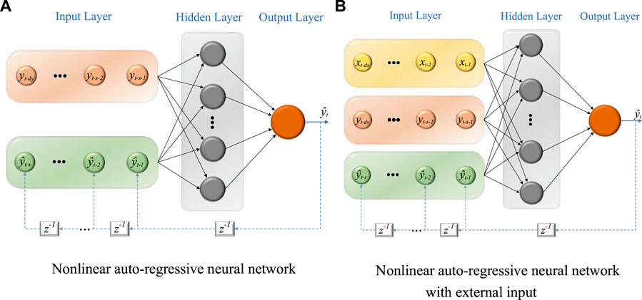
FIGURE 1. Two kinds of neural network structure, where ${\mathit{z}}^{-1}$ is the unit time delay. (A) Nonlinear auto-regressive neural network. (B) Nonlinear auto-regressive neural network with external input.

The NARNN model is primarily concerned with historical series of the target variables as shown in Eq. 12. The information carried by exogenous inflow data is ignored in this modeling process, and then NARXNN model is proposed to make use of this information. The NARXNN can be formulated as follows:

$\begin{array}{c}{\widehat{y}}_t=\mathcal{N}\left(\begin{array}{c}{\widehat{y}}_{t-1},{\widehat{y}}_{t-2},\cdots ,{\widehat{y}}_{t-s},y_{t-s-1},\\ \cdots ,y_{t-d_y},x_{t-1},\cdots ,x_{t-d_x}\end{array}\right),\end{array}(13)$

Where $\left[x_{t-1},\cdots ,x_{t-d_x}\right]$ is a matrix consisting of exogenous input variables, the dimension of $x$ depends on the quantity of exogenous input variables, and $d_x$ is the maximum delay index of exogenous input variables. The structure of NARXNN is different from the NARNN slightly, mainly with the addition of several extra inputs. The structure of NARXNN is presented as Figure 1B.

The two neural networks, NARNN and NARXNN, update weights in each layer by using the Bayesian regularization backpropagation algorithm (MacKay, 1992). Training samples are shown as following set, $D=\left\{\left({\overline{x}}_1,{\overline{y}}_1\right),\left({\overline{x}}_2,{\overline{y}}_2\right),\cdots ,\left({\overline{x}}_N,{\overline{y}}_N\right)\right\}$, where ${\overline{x}}_i\left(i=\mathrm{1,2},\cdots ,N\right)$ and ${\overline{y}}_i\left(i=\mathrm{1,2},\cdots ,N\right)$ represent the input and output of the neural network, respectively. Given a neural network, called $\mathcal{M}$, let $g\left(x;w,\mathcal{M}\right)$ be the response of network $\mathcal{M}$ with respect to the input $x$, and $w$ denotes the weight of network. The optimal parameters can be achieved by minimizing the quadratic cost function:

$\begin{array}{c}{E}_D={\displaystyle \sum }_{i=1}^N{\left[g\left({\overline{x}}_i;w,\mathcal{M}\right)-{\overline{y}}_i\right]}^2.\end{array}(14)$

The objective function is extended from $F=E_D$ to $F=\alpha E_D+\beta E_w$ to prevent the overfitting. The regularization term $E_w$ is denoted as:

$\begin{array}{c}{E}_w={\displaystyle \sum }_n{\omega }_n^2.\end{array}(15)$

Note that $\alpha$ and $\beta$ are unknown parameters of the objective function $F$. When $\alpha$ is larger, the accuracy of the model to the training samples is enhanced, and similarly when $\beta$ is larger, the generalization ability of the model is enhanced. The Bayesian regularization generally treats the network weights as random variables and the detailed methods for estimating the values of weights $w$, $\alpha$ and $\beta$ can be found in (Dan Foresee and Hagan, 1997).

NARNN and NARXNN are variants of ARMA together with neural network, combing both the dynamic and recurrent properties. Both methods do not require strict stationarity of the target time series. On the other hand, it is should be noted that NARXNN needs more reasonable computational cost (Cadenas et al., 2016).

2.3 The selection of features

Feature selection is of vital importance to improve the performance of the model, especially whose predictions depend on a number of extrinsic inputs to some extent. Excellent choices of inputs not only help to provide accurate results, but also speed up calculations and reduce the number of sensor installations, all of which lead to operational cost savings. The SVM-RFE combined with clustering method proposed in this study ranks the features of the continuous processes based on backward elimination.

The first thing worth noting is that the support vector machine classifier achieves the distinction between two classes by searching for the optimal hyperplane in a high-dimensional space (Rakotomamonjy, 2003). For the binary classification problem with training data set $\left\{\mathit{X},\mathit{Y}\right\}$, where $\mathit{X}\in {\mathbb{R}}^n$ are the features and $\mathit{Y}\in \left\{-\mathrm{1,1}\right\}$, there exists a hyperplane or decision function of the following form.

$\begin{array}{c}f\left(\mathit{X}\right)=\langle \mathit{w},\Phi \left(\mathit{X}\right)\rangle +b,\end{array}(16)$

Where $\Phi \left(\mathit{X}\right)$ refers to the mapping relationship from features $\mathit{X}$ to the high dimensional space. The parameters $\left(\mathit{w},b\right)$ are determined by minimizing the weights and the distance of each misclassified data to the hyperplane, before which the features $\mathit{X}$ need to be normalized. The optimization problem can be written as:

$\begin{array}{c}\underset{\mathit{w},\mathit{\xi }}{\min }\frac{1}{2}{\Vert \mathit{w}\Vert }^2+C{\displaystyle \sum }_{k=1}^m{\mathit{\xi }}_k^2,\end{array}(17)$

$y_{k}f\left({\mathit{x}}_k\right)\ge 1-{\mathit{\xi }}_k$

$\mathrm{s}.\mathrm{t}{y}_k\in \mathit{Y},{\mathit{x}}_k\in \mathit{X}\mathrm{f}\mathrm{o}\mathrm{r}\forall k$

Where $C$ is used as a penalty factor to weigh the importance of misclassification. SVM-RFE compares the impact of different remaining subsets on the classification by backward elimination of features, with the aim of preserving the subset of features that are most beneficial to the classification. The ranking of features is achieved through multiple iterations of elimination in the above work until the remaining feature subset is empty, and the criterion of elimination at each step for a given feature $i$ can be expressed as:

$\begin{array}{c}{R}_c\left(i\right)=\left|\mathbf{\nabla }{\Vert {\mathit{w}}^{\left(i\right)}\Vert }^2\right|,\end{array}(18)$

Where $\mathbf{\nabla }$ denotes the weight difference between the previous subset and the one whose $i^{th}$ feature is eliminated. The feature that minimizes $R_c$ will be removed after one round of loops, which means that the remaining feature subset has the least difference in classification performance from the feature subset containing the removed feature. It is worth mentioning that SVM-RFE was widely used in feature selection for binary classification problems, while it was rarely used in continuous classification problems.

In practical industrial processes, the variation in feature values often leads to continuous variation in the output. This begs a question that needs to be addressed. When each output point is treated directly as a separate label, the volume of the feature set corresponding to each label is so small that each feature set does not have the ability to characterize a specific label. Therefore, such continuous processes cannot be directly classified as a multi-label feature classification problem. In order to rank the features for this type of data, this study proposed SVM-RFE combined with clustering algorithm, as shown in Figure 2.

FIGURE 2

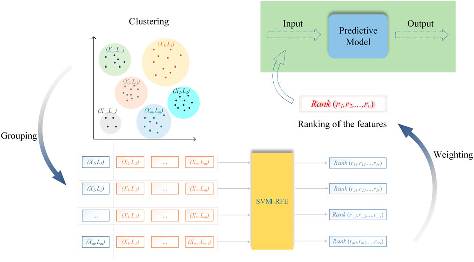
FIGURE 2. SVM-RFE combined with clustering algorithm for sequential feature ranking.

The successive outputs are first clustered to form new classes, and thus similar outputs can be grouped into homogeneous classes to enhance the differences between the new classes, e.g., $\left\{y_1,y_2,\cdots ,y_n\right\}\to \left\{L_1,L_2,\cdots ,L_m\right\},n\gg m$. The features corresponding to the same type of label are also merged into the same group, e.g., $\left\{x_1,x_2,\cdots ,x_n\right\}\to \left\{X_1,X_2,\cdots ,X_m\right\},n\gg m$. In this way, the original problem is successfully transformed into a multi-label feature classification problem. When SVM is used for multi-classification problems, it is usually transformed into a series of binary classification problems that are handled separately and then summarized for the final result. The new data set $\left\{\left(X_1,L_1\right),\left(X_2,L_2\right),\cdots ,\left(X_m,L_m\right)\right\}$ is partitioned using the so-called the one-versus-all method, and subsequently the features are individually ranked using SVM-RFE. The final summary of the ranking results for each group is ${\mathcal{R}}_{m\times v}$ as shown in Eq. 19.

$\begin{array}{c}\mathcal{R}=\left(\begin{array}{c}{\mathcal{R}}_1\\ ⋮\\ {\mathcal{R}}_m\end{array}\right)=\left(\begin{array}{ccc}{r}_{11}& \cdots & r_{1v}\\ ⋮& \ddots & ⋮\\ r_{m1}& \cdots & r_{mv}\end{array}\right),\end{array}(19)$

Where ${\mathcal{R}}_i\left(i=1,\cdots ,m\right)$ represents the ranking of the features that distinguish $\left\{X_i,L_i\right\}$ from the rest of dataset using SVM-RFE and the order, $r_{i1}$ to $r_{iv}$, is decreasing according to the importance of the $v$ optional features. For the ranking matrix $\mathcal{R}$, this research considers that the importance index of the same column is consistent, which unifies the weights assigned to the same column. Then the final ranking of all features, $\left\{r_1,r_2,\cdots ,r_v\right\}$, can be obtained by counting the frequency of each feature in each column.

In the final step, the model is trained by sequentially increasing the number of exogenous inputs to the model, depending on the importance of the features. Then, the appropriate training set is obtained by comparing the model test results under the AIC criterion. SVM-RFE combined with clustering algorithm migrates the feature ranking method for binary classification problems to a new application scenario and solves the problem of feature ranking for continuous processes. This approach implements feature selection while keeping the original data of the features intact and visually explaining the input variables selection.

3 Case studies

3.1 Performance evaluation index

In this study, MSE and R are used as the performance evaluation metrics of the model, which can be calculated as follows:

$\begin{array}{c}MSE=\frac{{\displaystyle \sum }_{t=1}^n{\left(y\left(t\right)-y_{et}\left(t\right)\right)}^2}{n},\end{array}(20)$

$\begin{array}{c}R=\frac{{\displaystyle \sum }_{t=1}^n\left(y\left(t\right)-\overline{y}\right)\left(y_{et}\left(t\right)-{\overline{y}}_{et}\right)}{\sqrt{{\displaystyle \sum }_{t=1}^n{\left(y\left(t\right)-\overline{y}\right)}^2}\sqrt{{\displaystyle \sum }_{t=1}^n{\left(y_{et}\left(t\right)-{\overline{y}}_{et}\right)}^2}},\end{array}(21)$

Where $y$ and $y_{et}$ refer to the true values of the system output and the estimated values of the prediction model, respectively; $\overline{y}$ and ${\overline{y}}_{et}$ are the mean values of $y$ and $y_{et}$. $n$ is the total number of evaluation samples. The smaller the MSE, the smaller the error of the model. R is in the range of $\left[\mathrm{0,1}\right]$, the closer it is to 1, the better the performance of model.

3.2 Operational cost index from wastewater treatment processes

3.2.1 Data processing

The data for the case study in this section mainly came from the wastewater treatment platform, BSM2-P Simulink simulation model, which adds the phosphorus treatment process based on BSM2. The actual collected inflow parameters (e.g., Qin: influent flow, SF: readily biodegradable substrate) were input into the simulation platform, and OCI was calculated every 15 min according to Eq. 22 based on the data collected from the simulation model.

$\begin{array}{c}OCI=3SP+AE+ME+PE+EC+\max \left(0,HE-7MP\right)+24MT-6MP,\end{array}(22)$

Where SP is the sludge production for disposal, AE is the aeration energy, ME is the mixing energy, PE is the pump energy, EC is external carbon addition, HE is the heating energy for increasing the temperature of the anaerobic digester, MP is the methane production, and MT is the metal salt to be added. A total of 50 days of data are illustrated in Figure 3, which has significant non-linearity. It should be noted that the reason for the negative OCI is that the methane produced in the water treatment process has a certain compensation for the operating cost.

FIGURE 3

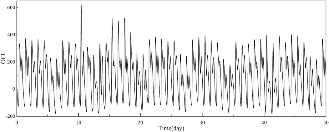
FIGURE 3. Operational cost index (OCI) over 50 days.

After the data of OCI and influent data were obtained, additional preparation for feature selection was required in addition to outlier removal and normalization. The operational cost of WWTP is closely related to the parameters of influent, but excessive parameters are not conducive to the further selection of features, so more preprocessing of the input data is required. Specifically, the selection of features practically implies exploring the correlation between exogenous inputs and target variables. The dataset with no or little change has little influence but will increase the subsequent computation, so that variables related to this kind of data need to be eliminated. Such problem can be solved by excluding feature arrays with variance less than a certain threshold. Furthermore, variables with strong linear correlation would make the SVM-RFE’s judgment of importance seem unreasonable. Therefore, some correlation analysis methods, such as Pearson correlation analysis, need to be used to isolate the variables with strong linear correlation before using SVM-RFE. The variables $\left\{t,S_F,S_I,S_{{PO}_4},X_I,Q_{in},S_{N_a}\right\}$ were finally selected in this study as the alternative input features for predicting OCI, and further ranked by using SVM-RFE combined with clustering algorithm. Table 1 shows the full overview of these variables.

TABLE 1

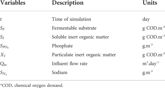
TABLE 1. Exogenous input variables related to OCI and descriptions.

To test the reliability of the method under different number of clusters, the diverse number of OCI clusters was set and the importance of each variable based on different number of clusters is presented in Figure 4. The results indicate that changes in the number of clusters over a wide range have some but little effect on the importance of exogenous variables, such that there is no change in the importance ranking of the variables. The decreasing ranking of variables importance is $\left\{S_F,Q_{in},X_I,S_I,S_{{PO}_4},S_{N_a},t\right\}$, where the importance indicators of $S_F$ and $Q_{in}$, $S_I$ and $S_{{PO}_4}$ are similar, respectively. It is worth noting that the importance of t behaves unusually at a clustering number of 1000, which is caused by the fact that the number of clusters is close to the raw data labels. As mentioned earlier, in order to accurately identify feature importance, classes with significant differences need to be generated by clustering.

FIGURE 4

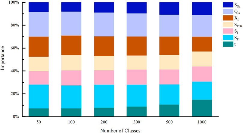
FIGURE 4. Importance of each variable to OCI with different number of clusters.

Generally, the model prediction accuracy will improve somewhat as the number of exogenous variables increases, but the rate of improvement is limited when the number of selected variables reaches a specific value. Fewer variables can be selected from alternative variables set to save computational power and avoid overfitting. Finally, according to the AIC criterion, $S_F$ and $Q_{in}$ were chosen as exogenous input variables in this study case.

3.2.2 Results and discussion

The OCI values for each time period were calculated using the data collected in the BSM2-P simulation model. A total of 4,799 samples from 50 days were retained. The sample set was split, with the data of the first week being the training set and the remaining as the testing set. Each model was applied to predict OCI over four steps ahead.

Figure 5 shows the prediction performance of four ARMA variant models on the last week of OCI values and compares them with the test set, respectively. As shown in Figures 5A,B, the ARMAX models based on two different algorithms are similar in overall prediction performance. Under relatively stable conditions, the predicted values of ARMAX model are in good agreement with some original data with linear characteristics. However, comparing the peak locations marked in Figures 5A,C, the ARMAX model has slightly worse performance. This mainly results from the fact that the linear model is not competitive for data predictions with significant nonlinearity. On the other hand, although the RELS algorithm takes into account the effect of residual information, the performance does not improve significantly compared to RLS. This is due to the limited effect provided by the residuals of the previous moment during the nonlinear change phase of the data.

FIGURE 5

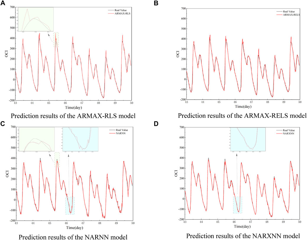
FIGURE 5. Prediction results of OCI for the last 7 days over four steps ahead. (A) Prediction results of the ARMAX-RLS model. (B) Prediction results of the ARMAX-RELS model. (C) Prediction results of the NARNN model. (D) Prediction results of the NARXNN model

Compared to the ARMAX model, the prediction values of the NARNN model displayed in Figure 5C are more in line with the real values. However, there are still deviations, as shown in the half-day period after the 46th day. The NARXNN model fits the real data better at the locations of the peaks, troughs, as well as under the other linear conditions as shown in Figure 5D. The residual distribution of the prediction results for the four variants is plotted in Figure 6. The NARXNN model produces a smaller span of error, which indicates the better prediction performance of the model.

FIGURE 6

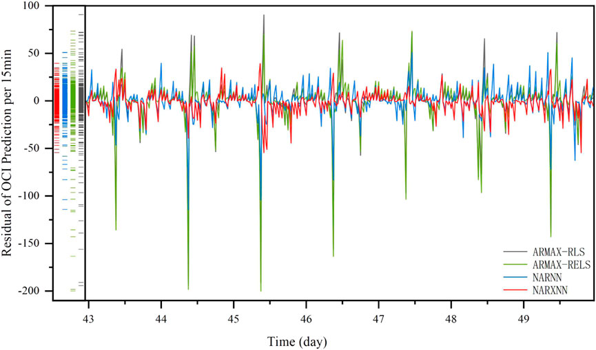
FIGURE 6. Prediction residual of OCI for the last 7 days over four steps ahead.

It is worth noting that the training of the neural network model has strong randomness. This can be solved by trials and errors. To well illustrate the performance of the proposed method, the results of NARNN and NARXNN are listed in Table 2, average values of which were calculated from the prediction more than 10 times. As can be seen from Table 2, the results are as follows: Compared with ARMAX-RLS, ARMAX-RELS and NARNN model, MSE of the NARX model is reduced by 78.50%, 79.52%, 50.75%, respectively, and R is improved by 0.89%, 0.96%, 0.28%. Based on the above results, it can be observed that NARXNN model has a better performance in predicting the wastewater treatment cost index.

TABLE 2

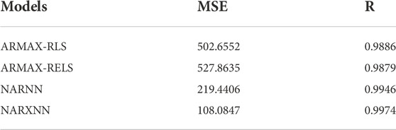
TABLE 2. Comparison of the Prediction Performance on OCI over four steps ahead.

3.3 Energy consumption from a full-scale steel plant

3.3.1 Data processing

The real data in this subsection, concerning energy consumption in the steel industry, were taken from University of California, Irvine (UCI). The data were collected from DAEWOO Steel Co., Ltd. in Gwangyang, South Korea. Energy consumption information for the industry is stored on the Korea Electric Power Corporation’s website (pccs.kepco.go.kr), and daily, monthly and annual data are computed and displayed. Figure 7 presents the data of energy consumption for every 15 min over a total of 50 days.

FIGURE 7

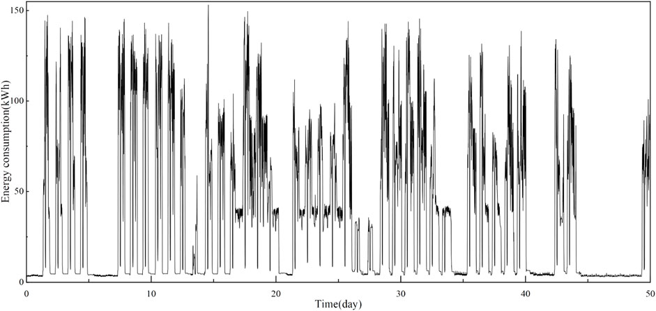
FIGURE 7. Operational cost index data for 50 days.

Obviously, the energy consumption data in this case are more non-linear due to the fact that they are collected directly from the actual steel plant. This data set even contains some coarse data or outliers, and exhibits significant dramatics over time. The data performance varied obviously at different time intervals, particularly from the 5th to the 7th day, the processes were stable relatively, while the stable processes changed completely from the 20th to the 21st day and from the 45th to the 50th day. The data from the 10th to the 15th day, the 15th to the 20th day and the 21st to the 27th day also changed completely with different fluctuating trends, all of which added the difficulty in the sequential modeling and predicting.

Table 3 lists the alternative exogenous variables provided in the data source file that present continuous numeric variation. Similarly, as mentioned earlier, the selection of model inputs is essential before building models with exogenous inputs. This work is based entirely on data relationships without considering the mechanism. The linear correlations between the variables in Table 3 were first examined by the Pearson correlation analysis, and there was a strong linear relationship between Lead. CRP and Lead. CPF. After removing Lead. CPF, the remaining four variables were analyzed for importance in this study case and the results are shown in Figure 8. It is noticeable that Lead. CRP and tCO2 have significantly higher importance indicators than the other two variables, and therefore Lead. CRP and tCO2 were identified as exogenous input variables for the prediction model of energy consumption in steel plant.

TABLE 3

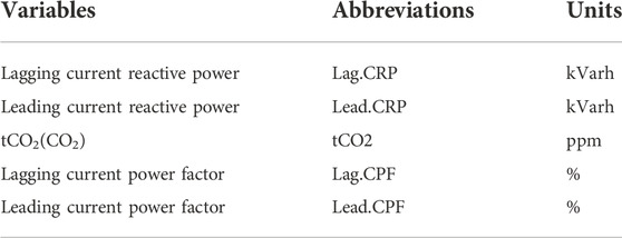
TABLE 3. Exogenous input variables related to the steel plant and descriptions.

FIGURE 8

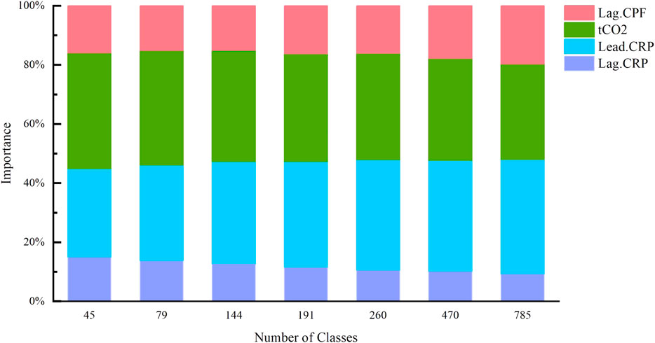
FIGURE 8. Importance of each variable to the energy consumption with different number of clusters.

3.3.2 Results and discussion

The dataset was split, with the first 7 days of data used as the training set and the remaining data used as the test set to evaluate the performance of each model for four steps ahead prediction. The prediction performance of the four variants of the ARMA model is shown in Figure 9, and in general, the prediction performance on real data all deteriorates compared to the prediction on the simulated data in the last study case. The main reason for this occurrence is still that the steel plant data set contains the rough data, as well as its own strong nonlinearity and sharp changes over time.

FIGURE 9

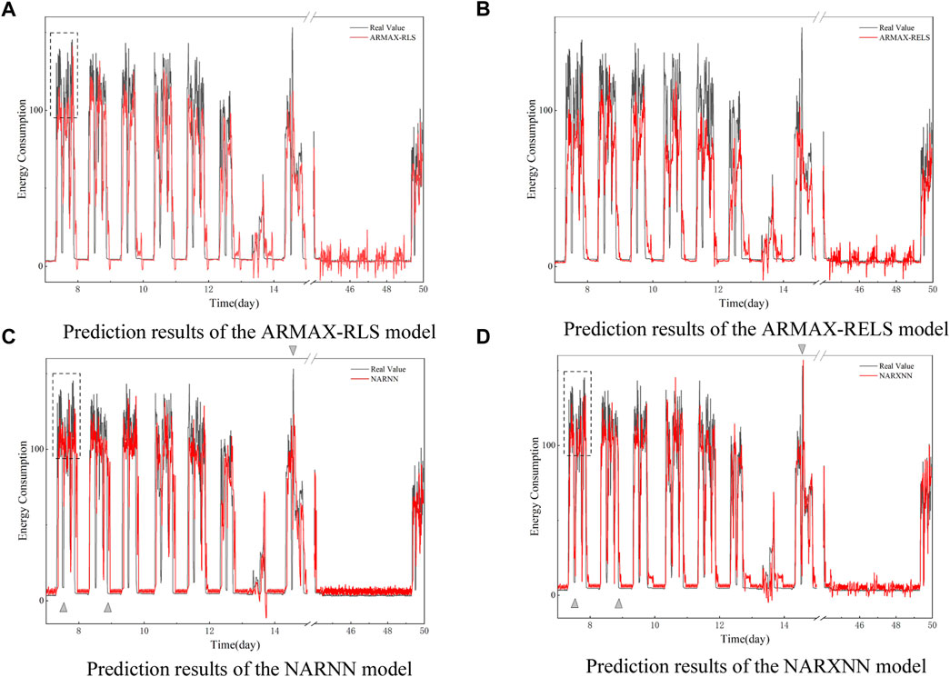
FIGURE 9. Prediction results of energy consumption over four steps ahead. (A) Prediction results of the ARMAX-RLS model. (B) Prediction results of the ARMAX-RELS model. (C) Prediction results of the NARNN model. (D) Prediction results of the NARXNN model

Nevertheless, in this study case, the neural network models perform much better than the general time series models. Specifically, the difference between the prediction results of two ARMAX models is small, and both have the tendency that the predicted data obviously cannot track the true data with high oscillation, as shown in the dashed rectangular box in Figure 9A. The predicted data from ARMAX-RELS are less overshooting compared to ARMAX-RLS when the energy consumption data change rapidly from a declining state to a flat state, as can be seen in the comparison of Figures 9A,B. On the contrary, two autoregressive neural network models perform much better in these issues.

As shown in Figures 9C,D, the results predicted by the two autoregressive neural network models oscillate less between the 44th and the 49th day, and the data perform more smoothly. However, the NARXNN model has a higher prediction accuracy than other models for parts with steep variations, such as the rising or falling edges indicated by the triangle symbol in the figure. Different from the NARXNN model, NARNN model performs even worse than ARMAX in these regions indicated by the triangle symbol, showing the positive impact of introducing exogenous inputs on the prediction results. Although the prediction for smooth data in the period from the 44th to the 49th day is slightly inferior to that of the NARNN model, the NARXNN still performs better overall.

The results are tabulated in Table 4 as follows: Compared with ARMAX-RLS, ARMAX-RELS and NARNN model, MSE of the NARX model is reduced by 28.46%, 18.85%, 45.36%, respectively, and R is improved by 6.40%, 1.79%, 14.02%. Based on the above results, it can be observed that NARXNN model has a better performance in predicting the energy consumption from a full-scale steel plant. It is worth noting that the performance of the NARNN model is quite different from that in the previous study case, which is mainly due to the lack of intervention from exogenous inputs. It is difficult for the general neural network model to predict the practical data with complex characteristics such as strong nonlinearity, strong volatility, and outliers in this case.

TABLE 4

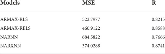
TABLE 4. Comparison of the Prediction Performance on Energy Consumption over four steps ahead.

4 Conclusion

Process monitoring of operational costs can benefit for the operational costs reduction and other financial budget management in industries. This paper provides a comparative analysis on the performance of four ARMA model variants (i.e., ARMAX-RLS, ARMAX-RELS, NARNN and NARXNN), using operational costs and energy consumption predictions as a baseline for real applications. In addition, a method based on SVM-RFE combined with clustering algorithm was developed to extract useful features that are important for the construction of the above-mentioned models and to provide a way to measure and explain how important the corresponding features are.

The analysis of the data and the evaluation of the prediction results lead to the following conclusions: The two time series models, ARMAX-RLS and ARMAX-RELS, have acceptable prediction performance under conditions where the data exhibit stable patterns. But if the predicted data have strong nonlinearities as well as irregular changes, two ARMAX models can only meet the minimum prediction needs. Compared to the other three variants, the NARXNN model achieves the most accurate prediction results in both study cases, due to the help of the neural network for nonlinear data prediction on the one hand and the choice of exogenous inputs on the other.

In future research, the method of feature selection will be further explored and the interpretability of the method will be enhanced. Another aspect is that predictive models will be further incorporated into control strategies for costs reduction in industrial processes.

Data availability statement

The original contributions presented in the study are included in the article/Supplementary Material, further inquiries can be directed to the corresponding author.

Author contributions

YL was responsible for the specific work of this manuscript. GF and YL collaborated to the analysis of the data and to the writing of the manuscript. DH guided the work of this manuscript. BC and HC reviewed the content of the paper.

Funding

This research was funded by the National Natural Science Foundation of China (62273151, 61873096, and 62073145), Guangdong Basic and Applied Basic Research Foundation (2020A1515011057, 2021B1515420003), Guangdong Technology International Cooperation Project Application (2020A0505100024, 2021A0505060001). Fundamental Research Funds for the central Universities, SCUT (2020ZYGXZR034). Yiqi Liu also thanks for the support of Horizon 2020 Framework Programme-Marie Skłodowska-Curie Individual Fellowships (891627).

Conflict of interest

The authors declare that the research was conducted in the absence of any commercial or financial relationships that could be construed as a potential conflict of interest.

Publisher’s note

All claims expressed in this article are solely those of the authors and do not necessarily represent those of their affiliated organizations, or those of the publisher, the editors and the reviewers. Any product that may be evaluated in this article, or claim that may be made by its manufacturer, is not guaranteed or endorsed by the publisher.

Supplementary material

The Supplementary Material for this article can be found online at: https://www.frontiersin.org/articles/10.3389/fenrg.2022.1073271/full#supplementary-material

References

Altıntaş, R. S., Kahya, M., and Ünver, H. Ö. (2016). Modelling and optimization of energy consumption for feature based milling. Int. J. Adv. Manuf. Technol. 86, 3345–3363. doi:10.1007/s00170-016-8441-7

CrossRef Full Text | Google Scholar

A. A. Ansari, S. Singh Gill, G. R. Lanza, and W. Rast (Editors) (2011). Eutrophication: Causes, consequences and control (Dordrecht: Springer Netherlands). doi:10.1007/978-90-481-9625-8

CrossRef Full Text | Google Scholar

Box, G. E. P., Jenkins, G. M., and Reinsel, G. C. (2008). Time series analysis: Forecasting and control. 4th Edition1st ed. Hoboken, New Jersey: John Wiley & Sons. doi:10.1002/9781118619193

CrossRef Full Text | Google Scholar

Cadenas, E., Rivera, W., Campos-Amezcua, R., and Cadenas, R. (2016). Wind speed forecasting using the NARX model, case: La mata, oaxaca, méxico. Neural comput. Appl. 27, 2417–2428. doi:10.1007/s00521-015-2012-y

CrossRef Full Text | Google Scholar

Car-Pusic, D., Petruseva, S., Zileska Pancovska, V., and Zafirovski, Z. (2020). Neural network-based model for predicting preliminary construction cost as part of cost predicting system. Adv. Civ. Eng. 2020, 1–888617013. doi:10.1155/2020/8886170

CrossRef Full Text | Google Scholar

Chan, D. Y.-L., Huang, C.-F., Lin, W.-C., and Hong, G.-B. (2014). Energy efficiency benchmarking of energy-intensive industries in Taiwan. Energy Convers. Manag. 77, 216–220. doi:10.1016/j.enconman.2013.09.027

CrossRef Full Text | Google Scholar

Dan Foresee, F., and Hagan, M. T. (1997). “Gauss-Newton approximation to Bayesian learning,” in Proceedings of International Conference on Neural Networks (ICNN’97), Houston, TX, USA, April 1997 (IEEE). doi:10.1109/ICNN.1997.614194

CrossRef Full Text | Google Scholar

De Gooijer, J. G., and Hyndman, R. J. (2006). 25 years of time series forecasting. Int. J. Forecast. 22, 443–473. doi:10.1016/j.ijforecast.2006.01.001

CrossRef Full Text | Google Scholar

Deng, H., Yang, K., Liu, Y., Zhang, S., and Yao, Y. (2021). Actively exploring informative data for smart modeling of industrial multiphase flow processes. IEEE Trans. Ind. Inf. 17, 8357–8366. doi:10.1109/TII.2020.3046013

CrossRef Full Text | Google Scholar

Ding, F. (2010). Several multi-innovation identification methods. Digit. Signal Process. 20, 1027–1039. doi:10.1016/j.dsp.2009.10.030

CrossRef Full Text | Google Scholar

Fang, T., and Lahdelma, R. (2016). Evaluation of a multiple linear regression model and SARIMA model in forecasting heat demand for district heating system. Appl. Energy 179, 544–552. doi:10.1016/j.apenergy.2016.06.133

CrossRef Full Text | Google Scholar

Guyon, I., and Elisseeff, A. (2003). An introduction to variable and feature selection. J. Mach. Learn. Res. 3, 1157–1182. doi:10.1162/153244303322753616

CrossRef Full Text | Google Scholar

Guyon, I., Weston, J., Barnhill, S., and Vapnik, V. (2002). Gene selection for cancer classification using support vector machines. Mach. Learn. 46, 389–422. doi:10.1023/A:1012487302797

CrossRef Full Text | Google Scholar

Han, Y., Zeng, Q., Geng, Z., and Zhu, Q. (2018). Energy management and optimization modeling based on a novel fuzzy extreme learning machine: Case study of complex petrochemical industries. Energy Convers. Manag. 165, 163–171. doi:10.1016/j.enconman.2018.03.049

CrossRef Full Text | Google Scholar

Hsu, D. (2015). Identifying key variables and interactions in statistical models of building energy consumption using regularization. Energy 83, 144–155. doi:10.1016/j.energy.2015.02.008

CrossRef Full Text | Google Scholar

Huang, K. Y., and Jane, C.-J. (2009). A hybrid model for stock market forecasting and portfolio selection based on ARX, grey system and RS theories. Expert Syst. Appl. 36, 5387–5392. doi:10.1016/j.eswa.2008.06.103

CrossRef Full Text | Google Scholar

International Energy Agency (2021). World energy outlook 2021, Paris: International Energy Agency. Available at; https://www.iea.org/reports/world-energy-outlook-2021.

Google Scholar

Jia, S., Yuan, Q., Cai, W., Li, M., and Li, Z. (2018). Energy modeling method of machine-operator system for sustainable machining. Energy Convers. Manag. 172, 265–276. doi:10.1016/j.enconman.2018.07.030

CrossRef Full Text | Google Scholar

Juberias, G., Yunta, R., Garcia Moreno, J., and Mendivil, C. (1999). “A new ARIMA model for hourly load forecasting,” in Proceedings of the 1999 IEEE Transmission and Distribution Conference (Cat. No. 99CH36333), New Orleans, LA, USA, June 1999 (IEEE), 314–319. doi:10.1109/TDC.1999.755371

CrossRef Full Text | Google Scholar

Kahraman, A., Kantardzic, M., Kahraman, M. M., and Kotan, M. (2021). A data-driven multi-regime approach for predicting energy consumption. Energies 14, 6763. doi:10.3390/en14206763

CrossRef Full Text | Google Scholar

Kun, Z., and Weibing, F. (2021). Prediction of China’s total energy consumption based on bayesian ARIMA-nonlinear regression model. IOP Conf. Ser. Earth Environ. Sci. 657, 012056. doi:10.1088/1755-1315/657/1/012056

CrossRef Full Text | Google Scholar

Li, M.-J., and Tao, W.-Q. (2017). Review of methodologies and polices for evaluation of energy efficiency in high energy-consuming industry. Appl. Energy 187, 203–215. doi:10.1016/j.apenergy.2016.11.039

CrossRef Full Text | Google Scholar

Liu, Y., Huang, D., Liu, B., Feng, Q., and Cai, B. (2021). Adaptive ranking based ensemble learning of Gaussian process regression models for quality-related variable prediction in process industries. Appl. Soft Comput. 101, 107060. doi:10.1016/j.asoc.2020.107060

CrossRef Full Text | Google Scholar

Liu, Y., Yang, C., Zhang, M., Dai, Y., and Yao, Y. (2020). Development of adversarial transfer learning soft sensor for multigrade processes. Ind. Eng. Chem. Res. 59, 16330–16345. doi:10.1021/acs.iecr.0c02398

CrossRef Full Text | Google Scholar

MacKay, D. J. C. (1992). A practical bayesian Framework for backpropagation networks. Neural Comput. 4, 448–472. doi:10.1162/neco.1992.4.3.448

CrossRef Full Text | Google Scholar

Rakotomamonjy, A. (2003). Variable selection using SVM-based criteria. J. Mach. Learn. Res. 3, 1357–1370. doi:10.1162/153244303322753706

CrossRef Full Text | Google Scholar

Shi, X., Huang, G., Hao, X., Yang, Y., and Li, Z. (2021). A synchronous prediction model based on multi-channel CNN with moving window for coal and electricity consumption in cement calcination process. Sensors 21, 4284. doi:10.3390/s21134284

PubMed Abstract | CrossRef Full Text | Google Scholar

Silva, V. L. G. da, Oliveira Filho, D., Carlo, J. C., and Vaz, P. N. (2022). An approach to solar radiation prediction using ARX and ARMAX models. Front. Energy Res. 10–822555. doi:10.3389/fenrg.2022.822555

CrossRef Full Text | Google Scholar

Vu, D. H., Muttaqi, K. M., Agalgaonkar, A. P., and Bouzerdoum, A. (2017). Short-term electricity demand forecasting using autoregressive based time varying model incorporating representative data adjustment. Appl. Energy 205, 790–801. doi:10.1016/j.apenergy.2017.08.135

CrossRef Full Text | Google Scholar

Wei, Y., Zhang, X., Shi, Y., Xia, L., Pan, S., Wu, J., et al. (2018). A review of data-driven approaches for prediction and classification of building energy consumption. Renew. Sustain. Energy Rev. 82, 1027–1047. doi:10.1016/j.rser.2017.09.108

CrossRef Full Text | Google Scholar

Wu, J., Cheng, H., Liu, Y., Huang, D., Yuan, L., and Yao, L. (2020). Learning soft sensors using time difference–based multi-kernel relevance vector machine with applications for quality-relevant monitoring in wastewater treatment. Environ. Sci. Pollut. Res. 27, 28986–28999. doi:10.1007/s11356-020-09192-3

PubMed Abstract | CrossRef Full Text | Google Scholar

Xiao, J., Li, Y., Xie, L., Liu, D., and Huang, J. (2018). A hybrid model based on selective ensemble for energy consumption forecasting in China. Energy 159, 534–546. doi:10.1016/j.energy.2018.06.161

CrossRef Full Text | Google Scholar