Strategy optimization of emergency frequency control based on new load with time delay characteristics

With the development of modern communication technology and the large number of new controllable loads connected to the power grid, the new controllable loads with flexible regulation characteristics can participate in the emergency frequency stability control. However, the communication state differences and spatial distribution characteristics of controllable load will affect the actual effect of frequency control. In this paper, an emergency frequency control method based on deep reinforcement learning is proposed considering the response time of controllable load shedding. The proposed method evaluates response ability for emergency control of controlled loads through load response time, controllable load amount and controllable load buses. Then, the controllable load with smaller response time is cut out preferentially to ensure rapid control, and the Markov Decision Process (MDP) is used to model the emergency frequency control problem. Finally, Rainbow algorithm of Deep Reinforcement Learning (DRL) is used to optimize the emergency frequency stability control strategy involving controllable load resources. The formation of emergency load shedding instruction is directly driven by high-dimensional operation state data after power grid failure, so that, the aim of minimizing the economic cost is achieved under the constraint of system stability. The effectiveness of the proposed method is verified in the IEEE 39-bus system.

1 Introduction

With the massive access of renewable energy and the interconnection of large-scale systems, the power grid has changed into a complex dynamic system, and it is difficult to establish accurate mathematical models for it (Fan et al., 2022; Ren et al., 2022). The increase of new energy penetration and the access of more electronic power equipment have brought new risks to the stability of frequency. When the power imbalance between the source and load occurs, it may lead to regional power outage and system collapse (Cao et al., 2021b,a; Wen et al., 2020). On the other hand, there are massive flexible loads on the load side, such as electric vehicles and temperature-controlled air conditioners (Zhang et al., 2022), which, in combination with modern communication technology, can be controlled when the system is in an emergency state. It can improve the flexibility and economy of the emergency frequency control of the power system. Therefore, it is of great significance for the stability of power grid that the new controllable load participates in the emergency frequency stability control.

At present, controllable load participation in the emergency frequency stability control has become one of the hot research topics in power system. Reference (Xu et al., 2018) proposed the comprehensive contribution index of interruptible load according to the total amount of load excision and the user excision, and obtained the load reduction strategy through optimization. In addition, the large proportion of controllable load and rapid continuous regulation capacity are used to improve the refinement of emergency control on the premise of ensuring safety and stability (Li and Hou, 2016). Some researchers cooperatively optimized the decentralized emergency demand response to obtain the optimal emergency frequency stability control strategy (Wang et al., 2020). However, the above research on the participation of controllable load in emergency frequency control only considers the basic indicators such as the total amount of the load shedding, the controllable load bus and the cost, and considers that the load removal is instantaneous. However, in practice, due to the differences in communication states and response speeds of controllable loads, different loads have different delay characteristics, which will produce different control effects. However, the influence of load delay characteristics on emergency frequency control is not considered in the above conferences.

In order to solve the problem of emergency frequency control in power system, current research methods mainly include response driven and event driven. The former calculated the load shedding amount and its action rounds offline/online according to the frequency deviation and frequency change rate of the inertia center. The latter usually carries out pre-control after monitoring the fault event to prevent the further expansion of the impact. The response-driven emergency frequency control will adjust the load reduction and action rounds in advance according to a certain operation scenario of the system (Terzija, 2006; Banijamali and Amraee, 2019; Li et al., 2020), which may be deviated from the actual operation scenario and affect the control effect. Most of the studies on event-driven load shedding are based on the optimization of the mathematical model of the power system (Xu et al., 2017, 2016), and the effect of load shedding strategy is closely related to the accuracy of the system model. The new power system has a high degree of nonlinearity and uncertainty, and it is difficult to establish an accurate mathematical model, which poses a challenge to obtain an accurate load shedding strategy.

In recent years, Machine Learning (ML) has been applied to power system stability control. It does feature mining based on data and does not need accurate mathematical model. In reference (Singh and Fozdar, 2019), support vector machine was used to evaluate the stability of the power system, and the optimal load shedding scheme was obtained according to the evaluation results. The extreme learning machine can also be used to train the load shedding prediction model offline and predict the actual load shedding online (Dai et al., 2012). The above traditional ML algorithm model is simple and relies too much on expert experience. Its control effect is affected by the size and quality of knowledge database, resulting in poor adaptability of the control effect of the model.

Combined with deep learning technology, DRL can realize high-dimensional feature extraction and direct learning of complex action space. Meanwhile, Deep Learning Q Network (DQN) and other algorithms improve the scalability and robustness of DRL, making it suitable for solving control problems of large-scale systems (Mnih et al., 2015; Schulman et al., 2017). Double DQN algorithm is used to effectively screen out the line breaking faults which can easily lead to power grid instability, and formulate emergency stability control measures (Zeng et al., 2020). In conference (Liu et al., 2018), it obtained the optimal shedding strategy to ensure the transient stability of power grid through Double DQN and Dueling DQN model analysis. In addition, DRL algorithm was also used to optimize the emergency frequency control strategy, and a variety of regulation methods were aggregated to reduce the stable frequency fluctuation (Chen et al., 2021). The above emergency control strategy is used to shed the whole line directly from the substation, without considering the influence of the new controlled load and its delay characteristics on the emergency control effect. At the same time, the stability and robustness of some algorithms are poor, and it is difficult to ensure the control effect of the model. Rainbow algorithm is based on DQN and it integrates a variety of improved algorithms. The model has superior stability and robustness, and has been widely used in the field of control and decision making (Hessel et al., 2017). Therefore, Rainbow algorithm is adopted in this paper to optimize the control strategy for emergency control involving controllable load considering delay characteristics.

In order to solve the above problems, this paper proposes an emergency frequency control method based on deep reinforcement learning Rainbow algorithm that considers the delay characteristics of the controlled load. According to the different delay characteristics, the new controllable load resources are modeled and aggregated to form an emergency control process in which the new controllable load is graded, and the load with smaller control delay is preferentially removed to ensure rapid removal. Finally, the deep reinforcement learning Rainbow algorithm model is used to optimize the emergency frequency control strategy, suppress the frequency drop depth of the system, reduce the deviation of the stable frequency, and reduce the control cost as much as possible.

2 Emergency frequency control with new controllable load participation

2.1 Mathematical description of power grid emergency frequency stability control

In frequency stability analysis of power systems, the frequency of each generator oscillates around the inertial center of the system. When the system is stable, the frequency of each generator will eventually approach the center of inertia frequency of the system. The center of frequency inertia fCOI is defined as follows:

$f_{\text{COI}}=\sum _{j=1}^m\left(H_j{f}_j\right)/\sum _{j=1}^m{H}_j(1)$

where m is the number of generators, H_j and f_j are the inertia time constant and frequency of generator bus j.

Due to the complexity of components in large power systems, the emergency frequency control problem is the highly nonlinear optimal decision problem. The mathematical model is adopted:

$\min F=\left|f_{\text{tem}}-f_{\text{tem}\text{.set}}\right|+\lambda \sum _{j=1}^m{P}_{\text{sl}j}(2)$

$x_t=g\left(x_t,y_t,d_t,a_t\right)(3)$

$0=h\left(x_t,y_t,d_t,a_t\right)(4)$

$x_t^{\min }\le x_t\le x_t^{\max }(5)$

$y_t^{\min }\le y_t\le y_t^{\max }(6)$

$a_t^{\min }\le a_t\le a_t^{\max }(7)$

where f_tem is the center stable value of the frequency inertia, f_tem. set is the preset frequency inertia of the center steady-state threshold, P_slj is the load shedding amount of bus j, λ is the weight coefficient, x_t is the state variable of the power grid, such as the angle and angular velocity of the generator rotor, y_t is the output variable of the power grid, such as the voltage of each bus, a_t is the control variable of the power grid, such as the emergency control to cut off generators or loads, d_t is a disturbance or fault that may occur in the power grid.

2.2 The aggregate modeling of new controllable load with delay characteristics

New power loads are constantly being integrated into new power systems, and demand-side loads are becoming more and more diversified, such as typical new loads such as electric vehicles, temperature-controlled air conditioning and intelligent buildings. These new loads have strong controllability, large volume and obvious time and space distribution characteristics, which can participate in emergency frequency stabilization control.

For different loads, the load amount is different, and their delay characteristics are different. In this paper, delay time refers to the time required from the decision of the control center to cut off the load from the main network, including the decision time of the control center, communication time and load response time. The delay time t_i of load bus i can be described as:

$t_i=t_{i,\text{dec}}+t_{i,\text{down}}+t_{i,\text{res}}(8)$

where ${t_i}_{\text{,dec}}$ is the decision time shedding the load i for the control center, ${t_i}_{\text{,down}}$ is the time required for the communication module to send the command to load i, ${t_i}_{\text{,res}}$ is the response time of load i.

The difference of the delay characteristics of controllable loads affects the effect of emergency frequency control, which is one of the important factors for the participation of controllable loads. Different from the traditional load, the time and space distribution characteristics of the controllable load slows down its control speed. Then, the drop depth of system frequency is increased. The spatial location of the load is dispersed, and the load granularity is small, so it is difficult to adjust by the traditional method. For different loads, it is necessary to establish models according to the location, the amount and the delay time of controllable loads. The modeling results are shown in Table 1.

TABLE 1

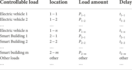
TABLE 1. Modeling results of controllable load with delay characteristics.

In actual control, because the single load amount of the new load is small and the loads is numerous, modeling only the single load with delay characteristics will lead to too large amount of resource data, which is difficult to deal with. In order to optimize the strategy more conveniently, the modeled controllable loads should be aggregated, that is, it should be graded according to the control delay, and the controllable loads of the same level should be aggregated. At the same time, in order to ensure the security, the delay time of this stage is taken as the maximal actual control delay of this stage of load. Although this method has some errors, it can reduce the difficulty of model building under the premise of considering the influence of load delay characteristics. Therefore, the aggregate modeling process of controllable load is shown in Figure 1.

FIGURE 1

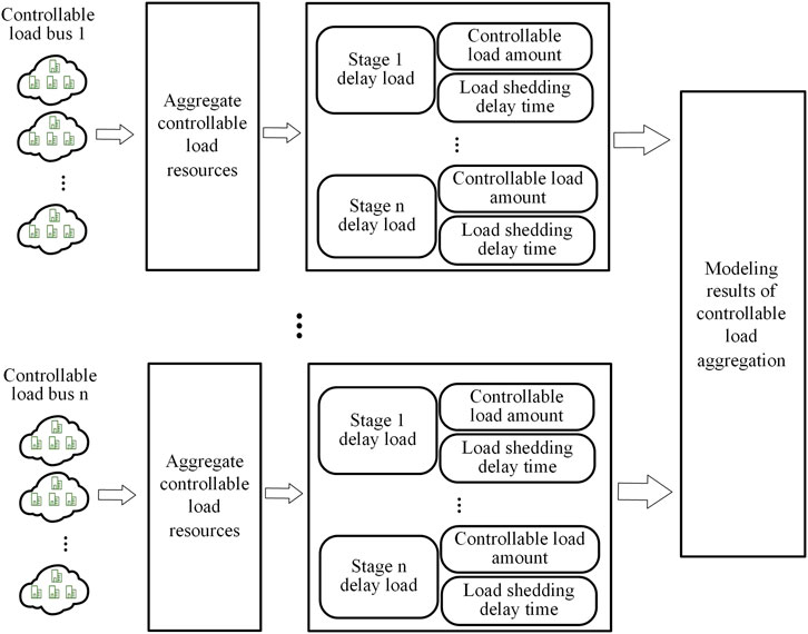
FIGURE 1. Controllable load aggregation modeling process.

After aggregation, a hierarchical aggregate controllable load of multiple buses is formed. The model is also composed of load location, load amount and load delay time. The result is shown in Table 2.

TABLE 2

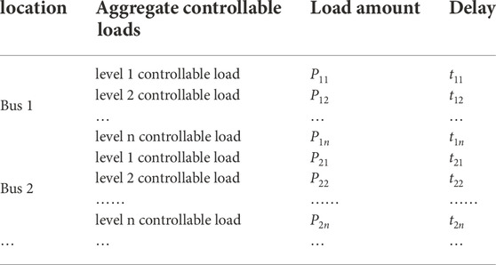
TABLE 2. Results of controlled load aggregation.

2.3 The process of emergency frequency control with new controllable load participation

In order to uniformly control the new controllable load with spatial distribution and delay characteristics, the controllable resource control process should be divided into uplink and downlink parts, and the control center and controllable load resources should be connected. The controllable resource control process starts with the control center, including the upstream controllable load aggregation modeling results, power grid fault perception and downlink control instructions. The control process is shown in Figure 2.

FIGURE 2

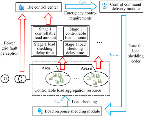
FIGURE 2. Emergency control process diagram of controllable load resources.

After modeling the new controllable loads of different buses with delay characteristics, the modeling results are sent to the control center. According to the information of controllable load resources, the control center is trained off-line to obtain the emergency frequency stability control model which can adapt to the current load state.

The control center monitors the power grid operation data in real time through the power grid fault perception. Once fault information or abnormal operation state of the power grid is found, the power grid operation state data will be put into the off-line training model to obtain the load shedding control instruction. After that, it transmits information through the control instruction delivery module to issue control actions to the controllable load resources on the demand side. The controllable load resources in each area complete the load shedding action response through the corresponding control components.

The new emergency control considering the controllable load resources is to implement cluster control on the controllable load before the traditional load shedding initial action, so as to avoid the whole line shedding caused by the traditional UFLS device. Therefore, the initial action of the new controllable load should take precedence over the traditional load shedding device, that is, the action frequency threshold of the controllable load control should be greater than the traditional initial action frequency threshold. When the system has power shortage, the method can quickly remove part of the new controllable load, achieve the purpose of load shedding in advance to restore the system frequency, without touching the traditional load shedding device. By controlling the aggregated new controllable load resources, the frequency recovery goal is achieved and the economy is higher than that of the traditional UFLS.

3 Deep reinforcement learning rainbow algorithm

The basic framework of Rainbow algorithm is the DQN algorithm. Therefore, this section first briefly introduces the DQN algorithm, and then explains the improvements and advantages of the Rainbow algorithm used in this article on its basis.

3.1 Deep learning Q network algorithm

The DQN algorithm uses deep neural networks to effectively extend the traditional tabular Q learning algorithm, which is a typical deep reinforcement learning algorithm. When training with the traditional Q learning method, it is necessary to use the Q table to record the status, action and corresponding Q value of each training sample, and the high-dimensional state and control action will cause the Q table to be too large and difficult to save. In order to solve the problem that it is difficult to deal with high-dimensional state space and control action set, the neural network is used to achieve direct prediction of Q values in the DQN method. This enables Q function to directly use the observed continuous states as input variables, which improves the ability of DQN to deal with complex problems. The process of using neural network to update Q value in DQN method can be described as:

$\begin{array}{ll}\hfill Q\left(s_t,a_t;{\theta }_t\right)& =Q\left(s_t,a_t;{\theta }_t\right)+\alpha \left(r_t+\gamma {\max }_{a_{t+1}}Q\left(s_{t+1},a_{t+1};{\theta }^{-}\right)\right.\hfill \\ \hfill & \left.-Q\left(s_t,a_t;{\theta }_t\right)\right)\hfill \end{array}(9)$

where Q (s_t, a_t; q_t) is the Q value function for evaluating the action a_t taken by the neural network under state s_t, θ_t is the neural network parameter of the evaluation network, r_t is the immediate reward value of the action, θ⁻ is the neural network parameters of the target network, α is the learning rates, γ is the attenuation coefficient.

The target network is the stage replica of the evaluation network in the learning process. The two neural networks complete the iteration of Q value together, which makes the iteration process more stable and improves the convergence of the algorithm. After the iteration of Q value, DQN trains the evaluation network according to the difference of Q value before and after the iteration, which is called time difference deviation, and the expression is shown as follows:

$H=r_t+\gamma {\max }_{a_{t+1}}Q\left(s_{t+1},a_{t+1};{\theta }^{-}\right)-Q\left(s_t,a_t;{\theta }_t\right)(10)$

The loss function L (θ_t) during the training of evaluation network is:

$L\left({\theta }_t\right)=H^2(11)$

In order to improve the learning efficiency of DQN, two methods are usually adopted: experience replay and regular target network correction. First of all, neural network training requires independent input samples, while Markov decision process can only produce continuous procedural samples. To this end, DQN sets up an experience playback mechanism to shuffle the procedural samples, and specially stores the historical experience data and learns from it repeatedly, so as to update the policy. In addition, in order to avoid the divergence of neural network caused by unstable training, DQN adopts the method of target network, that is, it sets two independent neural network models: target network and evaluation network, which have the same structure but different parameters. The evaluation network constantly learns new samples to update parameters, which is fast, while the target network parameters are updated periodically by replication evaluation network parameters, which is slow. This method can effectively improve the stability of DQN algorithm training.

3.2 Rainbow algorithm

Although the traditional DQN algorithm can also solve the problem of emergency frequency control strategy, sometimes there are some problems such as poor generalization effect and difficult convergence of the model. These problems are mainly caused by the shortcomings of the algorithm itself, which is difficult to be improved by adjusting parameters and model design. Using its improved Rainbow algorithm can effectively accelerate the training process, and make the emergency frequency control strategy more stable and effective, so as to solve the above problems.

The Rainbow algorithm used in this paper is based on DQN and integrates three types of improved algorithms: priority playback caching mechanism, Double DQN and Dueling DQN.

3.2.1 Priority playback caching mechanism

In the DQN algorithm, the playback cache mechanism uniformly filters data from the cache pool and is used to evaluate the training of the network. However, it fails to measure the quality of samples, resulting in some important data not being selected quickly, which makes the training efficiency of the evaluation network low. There is a large gap between the output value of some data and the target value, which makes it difficult to train the network successfully. Therefore, the priority of its filtering should be increased. The priority playback cache mechanism determines the probability of sampling according to the time difference deviation of each sample. In order to make the sample access more efficient, the algorithm also introduces sum-tree structure to store the sample and its corresponding priority, which is shown as:

$P_{\text{sum},t}\propto {\left|r_t+\gamma {\max }_{a_{t+1}}Q\left(s_{t+1},a_{t+1};{\theta }^{-}\right)-Q\left(s_t,a_t;{\theta }_t\right)\right|}^{\omega }(12)$

where P_sum,t is the probability that the sample will be sampled, ω the influence degree of time difference deviation on sampling probability.

In the priority playback cache mechanism, M experience samples are selected from the experience pool according to the priority to train the neural network. The loss value is used to determine the degree of priority learning. The larger the error is, the larger the space for the prediction accuracy to rise, and the higher the priority of the sample is, as shown in Figure 3.

FIGURE 3

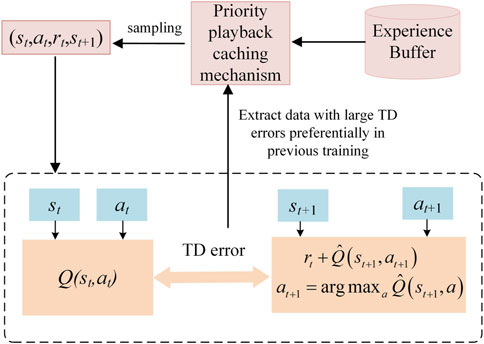
FIGURE 3. Schematic diagram of priority playback caching mechanism.

In fact, using a priority playback cache mechanism not only changes the process of filtering data, but also changes the method of parameter update. Therefore, it not only changes the distribution of selected data, but also changes the training method of the network. The priority playback cache mechanism extracts samples with larger time difference deviation more frequently, reduces the number of samples needed to evaluate the convergence of the network, significantly speeds up the convergence speed of the algorithm, and improves the learning efficiency of training.

3.2.2 Double deep learning Q network

Since the argmax function is included in the calculation formula of Q value, the estimation of Q value of DQN algorithm is often higher than the real value. If such overestimation is uniform, it will not affect the final optimal decision. However, the distribution of such overestimation in the environment is often complex and uneven, so different degrees of overestimation will lead to the final decision can only converge to the suboptimal solution instead of the optimal solution. The algorithm of Double DQN is proposed to solve this overestimation problem, which is an extension of DQN.

The difference between Double DQN and traditional DQN algorithms is mainly reflected in the estimation of the value of the next state. In DQN, the value estimation of the next state is done independently by the target Q network, and the target network outputs the Q value obtained by each action, and applies the action with the largest Q value to update formula. Double DQN uses two existing neural networks to improve the iterative rules for Q values, with the time difference bias H expression:

$\begin{array}{ll}\hfill H& =r_{t+1}+{\gamma }_{t+1}Q\left(s_{t+1},{\mathrm{a}\mathrm{r}\mathrm{g}\mathrm{m}\mathrm{a}\mathrm{x}}_{a_{t+1}}{Q}_{\theta }\left(s_{t+1},a_{t+1}\right);{\theta }^{-}\right)\hfill \\ \hfill & -Q\left(s_t,a_t;{\theta }_t\right)\hfill \end{array}(13)$

3.2.3 Dueling deep learning Q network

Dueling DQN makes a change in the upper layer of the neural network output layer and divides the original output Q value into two parts, one is the value evaluation of the state and the other is the value evaluation of different actions. Two parts share parameters at the front end of the neural network, and only perform shunt when calculating their respective values. The state value $V\left(s_t\right)$ in the first part represents the value of the state, while the action dominance value $A\left(s_t,a_t\right)$ in the second part removes the influence of the state and calculates the value of each action separately. The final output Q value can be calculated as:

$Q\left(s_t,a_t\right)=V\left(s_t\right)+A\left(s_t,a_t\right)(14)$

Dueling DQN provides a more accurate grasp of the environment by assessing the state and action separately, making decisions more realistic, as shown in Figure 4.

FIGURE 4

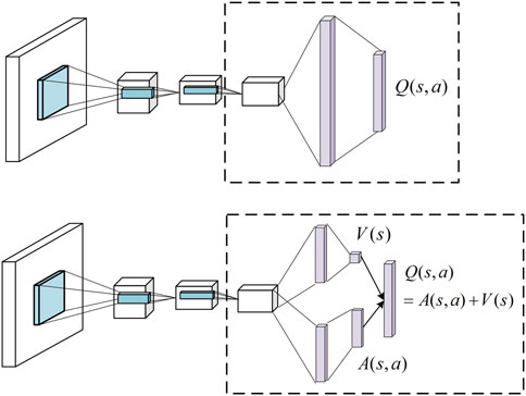
FIGURE 4. Schematic diagram of Dueling DDQN.

4 Emergency frequency control model based on deep reinforcement learning

When Rainbow algorithm is applied to the emergency frequency control of the power system, the emergency load shedding instructions can be directly generated by high-dimensional state data of power system, which avoids the disadvantages of traditional methods such as complex optimization and poor application effect. The power system emergency frequency control problem is formulated as MDP process, which has the elements of state, action and reward. In the process of MDP, the agent perceives the current system state and performs actions on the environment according to strategies, so as to change the state of the environment and get instant payoff. The accumulation of instant payoff over time is called reward. Thus, the MDP process combines the state space, action space and reward function of the emergency frequency control problem into a closed-loop whole. The MDP process of deep reinforcement learning algorithm is designed according to the mathematical model of the problem. The state control, action space and reward function correspond to each part of the mathematical model of the emergency control. Therefore, this paper introduces the mathematical description of emergency frequency stability control.

4.1 State space

In MDP, the state s_t represents the feedback of the environment to the agent, that is, the impact of the action of the previous step on the environment. This paper believes that the frequency stability of the power system is closely related to the active power of the generator, the load power and other factors, so the state space s_t is defined as:

$\begin{array}{ll}\hfill & s_t=s_1^t\cup s_2^t\cup s_3^t\cup s_4^t\hfill \end{array}(15)$

$\left\{\begin{array}{c}{s}_1^t=\left\{\begin{array}{cccc}\hfill f_1^t\hfill & \hfill f_2^t\hfill & \hfill \cdots \hfill & \hfill f_m^t\hfill \end{array},\right\}\hfill \\ s_2^t=\left\{\begin{array}{cccc}\hfill {\left(\text{d}f/\text{d}t\right)}_1^t\hfill & \hfill {\left(\text{d}f/\text{d}t\right)}_2^t\hfill & \hfill \cdots \hfill & \hfill {\left(\text{d}f/\text{d}t\right)}_m^t\hfill \end{array}\right\}\hfill \\ s_3^t=\left\{\begin{array}{cccc}\hfill P_{\text{e}1}^t\hfill & \hfill P_{\text{e}2}^t\hfill & \hfill \cdots \hfill & \hfill P_{\text{e}m}^t\hfill \end{array}\right\}\hfill \\ s_4^t=\left\{\begin{array}{cccc}\hfill P_{\text{l}1}^t\hfill & \hfill P_{\text{l}2}^t\hfill & \hfill \cdots \hfill & \hfill P_{\text{l}n}^t\hfill \end{array}\right\}\hfill \end{array}\right.(16)$

where ${f_i}^t$ is the frequency of generator bus i at time t, ${{\left(df/dt\right)}_i}^t$ is the frequency change rate of generator bus i at time t, ${P_{\text{e}i}}^t$ is the electromagnetic power of generator bus i at time t, ${P_{\text{l}j}}^t$ is the active load of the load bus j at time t.

4.2 Action space

For power system emergency frequency stabilization problems, the action is defined as removing a certain amount of load on multiple controllable load buses. At each action moment, the control action on each controllable load bus is defined as 0 (the controlled load is not shed) or 1 (a controlled load of σ amount is shed). Therefore, the action space is discrete, the dimensionality is 2ⁿ, where n is the number of load buses participating in emergency control.

4.3 Reward function

After an action is performed in a power system simulation environment, the model receives an immediate reward value to evaluate the corresponding state-action group at this time. For emergency frequency control problems, a larger reward value should be given if the action performed stabilizes the system frequency within the allowable range, keeps the system transient frequency nadir above the threshold, and shed less controllable load.

In order to quickly restore the system frequency to the allowable range, if the value of the frequency inertia center is still lower than the specified threshold in a certain period before the end of the simulation process, a large penalty value can be obtained. If the time does not reach the above moment, in order to keep the minimum frequency of the system higher than the threshold and remove less controllable load, the reward function consists of the following four parts:

1) The frequency inertia center deviation value of the system after the action;

2) The controllable load amount of shedding;

3) The penalty for crossing the threshold at the lowest point of the center of frequency inertia;

4) Invalid action penalty for removing unloaded buses.

Thus, the reward function r_t at time t can be defined as:

$r_t=\left\{\begin{array}{c}-200,if\left(t>T_{\text{tem}}\right)\text{\hspace{0.17em}and\hspace{0.17em}}\left(f\left(t\right)<f_{\text{tem}\text{.set}}\right)\hfill \\ {\lambda }_1\mathrm{\Delta }f\left(t\right)-{\lambda }_2\sum _{j=1}^n{P}_{\text{sl}j}-H_1-H_2\text{,\hspace{0.17em}otherwise\hspace{0.17em}}\hfill \end{array}\right.(17)$

$H_1=\left\{\begin{array}{c}-100,if\left(f\left(t\right)<f_{\min \text{.set}}\right)\hfill \\ 0,\text{\hspace{0.17em}otherwise}\hfill \end{array}\right.(18)$

$H_2=\left\{\begin{array}{c}-100,if\left({P_{\text{l}j}}^t=0\right)\text{\hspace{0.17em}and\hspace{0.17em}}\left(P_{\text{sl}j}\in a_t\right)\hfill \\ 0,\text{\hspace{0.17em}otherwise}\hfill \end{array}\right.(19)$

where T_tem is the value at a certain moment before the end of the simulation process, f_tem. set is the steady-state threshold of the frequency inertia center, $\mathrm{\Delta }f\left(t\right)$ is the deviation value of the frequency inertia center at time t, P_slj is the excision amount of load bus j, λ₁ and λ₂ are the coefficients of each part of the reward function, f_min. set is the threshold of the lowest point of the transient process frequency inertia center, H₁ is the penalty when the lowest point of the system frequency inertia center is less than the preset threshold, H₂ is the penalty when the load bus has been reduced to zero in the previous time step, and it still chooses the load shedding action.

The reward function design of deep reinforcement learning should combine the priori experience knowledge and automatic parameter search. Firstly, the priori experience about the emergency control problem is used to determine the approximate range of the coefficients of each part of the reward function. Secondly, once its rough range is determined, the model is automatically selected randomly in the range. The combination of selected parameters is used to train the model, and the combination with the best performance is selected as the coefficient of the reward function.

This reward function can quickly restore the system frequency to the allowable range, and the lowest frequency in the recovery process should not be lower than the threshold at the same time. It also ensures that the total amount of load shedding is small, and improve the economy.

5 Case study

In order to verify the effectiveness of the proposed method, Python and BPA simulation software are used to jointly build a deep reinforcement learning environment of IEEE 39-bus system, and Rainbow algorithm is used to solve the example. Tensorflow1.15 is used to build deep neural network in Python. The operating platform is Intel Core I5-11400H CPU, 16.00GB RAM, and RTX 3050.

5.1 Case data

In this paper, BPA is used to generate the failure scenario of IEEE 39-bus system. The generator model adopts the 6-order model. The load model is a mixed load model composed of constant impedance model and induction motor, both of which account for 50%. The failure scenario is that a generator loses part of the power, resulting in a certain power difference in the power system. The total simulation time is 40 s, and each cycle wave is a sampling point. In order to simulate fault states of different system and get enough samples, at the beginning of the simulation, one of the 10 generators is randomly selected to lose 0.5 p.u to 1 p.u of active power output. This random selection of fault location and fault size can improve the generalization ability of model. IEEE 39-bus topology is shown in Figure 5. In this paper, bus 3, 8, and 20 are considered as controllable load bus participating in emergency frequency control.

FIGURE 5

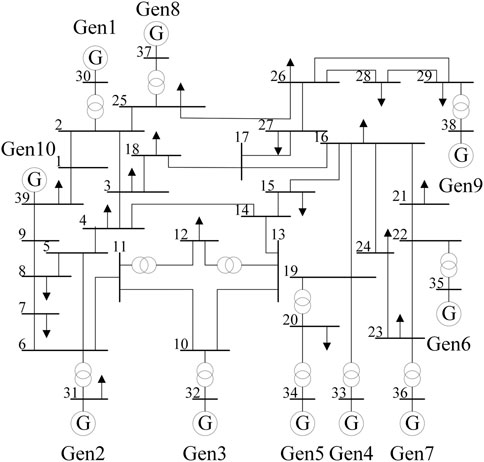
FIGURE 5. Topology of IEEE 39-bus.

In IEEE 39-bus system, the deep reinforcement learning state space is composed of the frequency deviation, frequency change rate, active power output of 10 generators and the remaining controllable load buses participating in load shedding, with a size of 33 dimensions. The action space is composed of the combined excision actions of three loads. The control action at each load bus is defined as 0 (the controlled load is not shed) or 1 (the controlled load of 50 MW amount is shed), and the size of the action space is 8 dimensions.

5.1.1 Two-stage action

Emergency frequency control is divided into two stages: emergency control action process and recovery action process. When the center of inertia of the system frequency is lower than 49.5Hz, the initial emergency control action starts, and then the time interval of each action is 0.5 s. Continuing operate until the frequency change rate of the center of inertia of the system is positive, that is, when the center of frequency inertia begins to rise, enter the second stage. In the second stage, the recovery action is performed with an interval of 5 s each time, and the action is continued until the frequency stability is reached.

5.1.2 Graded shedding polymerization load

Considering the different delay characteristics of the new controllable load, the load is divided into three levels according to the delay time. The delay time within 100 ms is level 1 load, the delay time between 100 and 200 ms is level 2 load, and the delay time between 200 and 300 ms is level 3 load. After aggregation modeling, the controllable load ratio of each bus and the load ratio of different delay levels are shown in Table 3.

TABLE 3

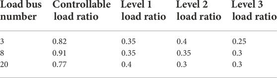
TABLE 3. Proportion of different grades of load.

For loads of the same delay level, the actual control delay is calculated according to the maximum value, so as to ensure that the actual frequency drop depth is less than or equal to the ideal frequency drop depth and avoid frequency instability. Therefore, after aggregation, it is considered that the actual delay of level 1 load is 100 ms, level 2 load is 200 ms, and level 3 load is 300 ms. In each bus, the delay is shed in ascending order.

In this paper, the delay difference of less than 100 ms is small, and the influence on the control effect can be ignored. Therefore, the load delay is divided into three levels. If the delay level is too coarse, the delay difference within the same level cannot be ignored. If the delay level is too fine, the strategy optimization is too complicated and unnecessary.

5.2 Model training process

In this paper, different experimental scenarios are set to train the proposed Rainbow algorithm. The size of the input layer of the neural network is 33 dimensions, which is the same as the dimension of the state space, and there are two 64-dimension hidden layers in the middle. The size of the output layer is 8 dimensions, which is the same as the dimension of the action space, and the activation function adopts ReLU.

During training, the strategy of ɛ-greedy search action is adopted to balance the relationship between exploration and utilization. It can prevent the agent from falling into the local optimal solution or not getting the optimal solution. Policy selection is defined as:

$a=\left\{\begin{array}{cc}\hfill \arg {\max }_{a}Q\left(s,a\right),\hfill & \hfill \epsilon \le {\epsilon }_0\hfill \\ \hfill \text{\hspace{0.17em}random,\hspace{0.17em}}\hfill & \hfill \epsilon >{\epsilon }_0\hfill \end{array}\right.(20)$

Where ɛ is the random number evenly distributed within the interval [0,1], ɛ₀ is the fixed value of the specified greedy policy, satisfying 0 ≤ ɛ₀ ≤ 1.

The ɛ₀ is small in the initial stage, which encourages DQN to explore more different load increase situations in the early stage of training, so as to avoid the problem of local optimum caused by insufficient exploration. With the progress of training, the value of ɛ₀ increases continuously and stabilizes at 0.95 finally, which requires DQN to learn and utilize the explored excellent strategies more in the later training period.

The training process of reinforcement learning model is the process of learning to obtain the maximum reward value. The reward change process in the training of this paper is shown in Figure 6.

FIGURE 6

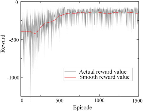
FIGURE 6. Change of reward value during training.

As can be seen from Figure 6, at the beginning of training, the agent randomly selects actions to explore the environment, because the data cache pool is not full and the ɛ₀ is small. Therefore, the reward value at this stage is low and there is obvious oscillation. When the data cache pool is full, the model starts to train, the reward increases with the training, and the effect of load shedding strategy gradually becomes better. After about 700 rounds of training, the reward reaches a high value, and then the change is small, and the model is basically trained.

In order to further show the process of model training, it is shown in Figure 7 that the change process of each round of shedding action step in the training process.

FIGURE 7

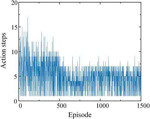
FIGURE 7. The number of excised movements in each training round.

As can be seen from Figure 7, at the early stage of training, the effect of load shedding is not ideal because the optimal strategy is not explored, so there are many action steps in each round. After training, the well-trained agent only needs to take a few actions in each round to achieve the stability condition.

5.3 Rainbow model test results

After the training, in order to test the robustness and adaptability of the Rainbow agent, it was tested in different scenarios. The test scenario is that one of the 10 generators loses 0.5 p.u to 1 p.u of active power output, and the load level is randomly selected as 90%, 95%, 100%, 105%, or 110%. The frequency control strategies for the three scenarios are shown in Table 4.

TABLE 4

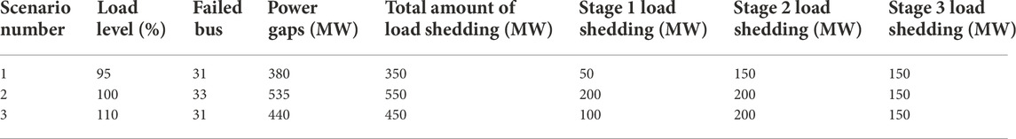
TABLE 4. Frequency control strategy in three scenarios.

As can be seen from Table 4, for various scenarios tested, the amount of load shedding is basically equal to the amount of power gaps, and the well-trained model can basically avoid overcutting or undercutting of load when applied online.

In order to further verify the superiority of the method, this paper compares the load shedding scheme obtained by the deep reinforcement learning Rainbow algorithm and the traditional UFLS algorithm, and Figure 8 shows the dynamic recovery process of frequency inertia center after the action of the two algorithms in scenario 2.

FIGURE 8

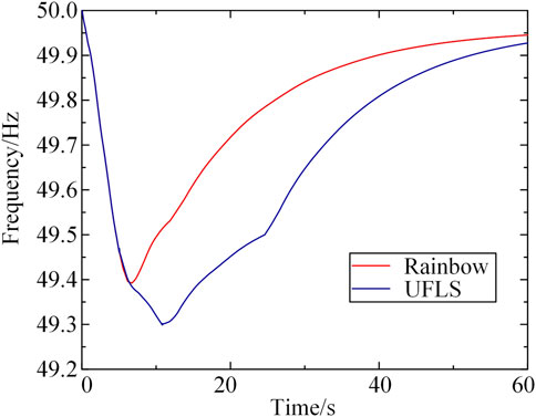
FIGURE 8. Curve of frequency inertia center after action of UFLS and Rainbow algorithm.

As can be seen from Figure 8, traditional UFLS is driven by multiple frequency stages, and the shedding action starts too slowly and is fixed, resulting in slow frequency recovery. However, Rainbow algorithm can effectively reduce the system frequency drop depth and speed up the process of frequency recovery. Within 10–60 s, the system frequency using Rainbow algorithm is much higher than that using UFLS, and the frequency recovery speed is accelerated. At the same time, when Rainbow algorithm is used, the lowest frequency of the system is around 49.4Hz, while the lowest frequency of the traditional UFLS algorithm is 49.3 Hz. It can be seen that the load shedding strategy in this paper can effectively improve the dynamic frequency nadir of the system and improve the frequency stability of the system.

5.4 Effect comparison of different deep reinforcement learning algorithms

In order to comprehensively compare the effect of the proposed algorithm with other DRL algorithms, Rainbow algorithm is compared with various improved DQN algorithms. Figure 9 shows the reward change process during training of different DRL algorithms.

FIGURE 9

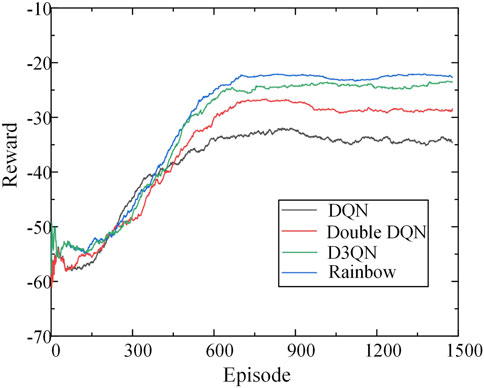
FIGURE 9. Reward value for DQN and its improved algorithm.

As can be seen from Figure 9, the traditional DQN algorithm is basically stable after 600 rounds of training, but its algorithm has poor optimization ability, and the reward value obtained is lower than that of its improved algorithm. After using the improved Double DQN and D3QN algorithms, the model converges after 700 rounds, and the training effect is improved compared with the DQN algorithm, and a better control strategy can be calculated. The Rainbow algorithm in this paper converges after about 800 rounds of training, at which point the model reward value exceeds that of other algorithms. As a result, the Rainbow algorithm is able to obtain higher reward values than other algorithms, and although the training time is longer, it obtains a better control strategy at the expense of this.

Meanwhile, in order to verify whether Rainbow algorithm maintains its superior performance in the test scenario, this paper randomly tests four different algorithms for 100 times, and the test scenario is the same as that in 5.3. The distribution of reward value obtained in the test is shown in Figure 10.

FIGURE 10

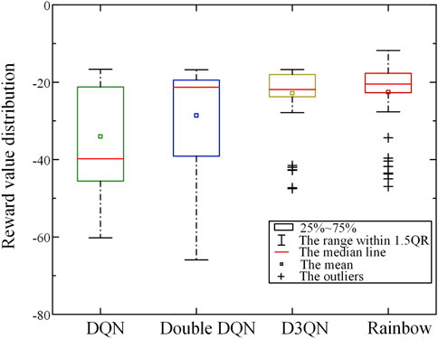
FIGURE 10. The distribution of reward values of different algorithms.

As can be seen from Figure 10, the reward value obtained by DQN and Double DQN fluctuates greatly in the random test scenario, and the overall reward is low. It indicates that the model fails to find the optimal strategy at this time, and the generalization ability is poor, and the effect is poor for some test scenarios. The reward value of D3QN algorithm in the test is significantly higher than that of the previous two, but there is still a certain gap compared with Rainbow algorithm in this paper. Rainbow algorithm with successful training can obtain good reward values in various test scenarios and obtain the optimal action strategy.

Compared with other DRL algorithms, Rainbow algorithm can make the system frequency return to stable state faster, and minimize the total load shedding amount at the same time. In order to show the test improvement effect more intuitively, Figure 11 shows the distribution of frequency inertia center values of system at a certain time before the end of simulation process after the implementation of random test strategy.

FIGURE 11

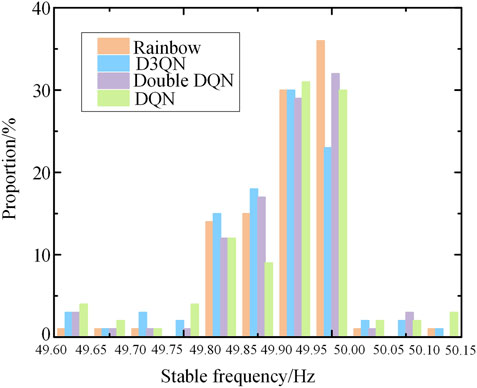
FIGURE 11. Frequency distribution at the time of system stability in different test scenarios.

As can be seen from Figure 11, the model trained by the deep reinforcement learning algorithm can basically restore the system frequency above 49.8 Hz under various test scenarios, ensuring the stability of the system. However, compared with other traditional DQN algorithms, Rainbow algorithm can make the stable frequency deviation smaller, which reflects the superiority of Rainbow algorithm.

6 Conclusion

Considering the complexity and uncertainty of frequency stability of the new power system, and the feasibility of the new controllable load participating in the emergency control, this paper established a new controllable load participating in the emergency frequency stability control method based on Rainbow algorithm. Through the design of different operation scenarios for experimental verification, the conclusion is as follows.

1) In this paper, it comprehensively evaluates the response delay time of the new controllable load, and classifies and aggregates the controllable load according to the different delay time. At the same time, the simplified model makes the controllable load more accurate and effective when participating in the emergency control, and avoids the error of shedding effect due to the communication difference and spatial distribution of the controllable resources.

2) The emergency frequency control algorithm based on deep reinforcement learning can effectively maintain the balance between the system frequency stability and the emergency control cost. By designing the reward function, the model can learn the effective control strategy with the minimum control cost. It avoids the shortcomings of the traditional algorithm such as easy over-cutting, under-cutting and poor economy. In this paper, Rainbow algorithm improved by DQN algorithm is adopted to avoid the shortcomings of traditional UFLS method, such as slow control speed, slow frequency recovery and excessive frequency drop. At the same time, compared with other DRL algorithms, the strategy obtained by the proposed algorithm is more excellent and the stable frequency deviation is smaller.

3) In the subsequent study, the random fluctuation of system load will be added to simulate a more realistic power system environment and test the generalization ability of this method. In addition, Rainbow algorithm adopted in this paper can only deal with discrete action space. It is hoped that deep reinforcement learning algorithm based on policy gradient can be applied to emergency frequency control in subsequent studies, and its ability to deal with continuous action space can enable more controllable loads to participate in emergency control.

Data availability statement

The original contributions presented in the study are included in the article/Supplementary Material, further inquiries can be directed to the corresponding author.

Author contributions

LS: conceptualization, methodology, software; YT: software, data curation, writing-original draft preparation; YW: visualization, investigation; WH: supervision; CY: validation; JY: funding acquisition.

Funding

This work was supported by the National Natural Science Foundation of China (52077059).

Conflict of interest

The authors declare that the research was conducted in the absence of any commercial or financial relationships that could be construed as a potential conflict of interest.

Publisher’s note

All claims expressed in this article are solely those of the authors and do not necessarily represent those of their affiliated organizations, or those of the publisher, the editors and the reviewers. Any product that may be evaluated in this article, or claim that may be made by its manufacturer, is not guaranteed or endorsed by the publisher.

References

Banijamali, S. S., and Amraee, T. (2019). Semi-adaptive setting of under frequency load shedding relays considering credible generation outage scenarios. IEEE Trans. Power Deliv. 34, 1098–1108. doi:10.1109/TPWRD.2018.2884089

CrossRef Full Text | Google Scholar

Cao, Y. J., Zhang, H. X., Xu, Q. W., Li, C. G., and Li, W. (2021a). Preliminary study on participation mechanism of large-scale distributed energy resource in security and stability control of large power grid. Automation Electr. Power Syst. 45, 1. doi:10.7500/AEPS2021021000

CrossRef Full Text | Google Scholar

Cao, Y. J., Zhang, H. X., Zhang, Y., and Li, C. G. (2021b). Event-driven fast frequency response control method for generator unit. Automation Electr. Power Syst. 45, 148. doi:10.7500/AEPS20210426006

CrossRef Full Text | Google Scholar

Chen, C., Cui, M., Li, F., Yin, S., and Wang, X. (2021). Model-free emergency frequency control based on reinforcement learning. IEEE Trans. Ind. Inf. 17, 2336–2346. doi:10.1109/TII.2020.3001095

CrossRef Full Text | Google Scholar

Dai, Y., Xu, Y., Dong, Z. Y., Wong, K. P., and Zhuang, L. (2012). Real-time prediction of event-driven load shedding for frequency stability enhancement of power systems. IET Gener. Transm. Distrib. 6, 914–921. doi:10.1049/iet-gtd.2011.0810

CrossRef Full Text | Google Scholar

Fan, S., Wei, Y. H., He, G. Y., and Li, Z. Y. (2022). Discussion on demand response mechanism for new power systems. Automation Electr. Power Syst., 1. doi:10.7500/AEPS20210726010

CrossRef Full Text | Google Scholar

Hessel, M., Modayil, J., Hasselt, H. V., Schaul, T., Ostrovski, G., Dabney, W., et al. (2017). . “Rainbow: Combining improvements in deep reinforcement learning,” in 32nd AAAI Conference on Artificial Intelligence, AAAI 2018, 3215–3222.

Google Scholar

Li, B. J., and Hou, Y. Q. (2016). Research of emergency load regulation for security and stability control. Power Syst. Prot. Control 44, 104. doi:10.7667/PSPC151194

CrossRef Full Text | Google Scholar

Li, C., Wu, Y., Sun, Y., Zhang, H., Liu, Y., Liu, Y., et al. (2020). Continuous under-frequency load shedding scheme for power system adaptive frequency control. IEEE Trans. Power Syst. 35, 950–961. doi:10.1109/TPWRS.2019.2943150

CrossRef Full Text | Google Scholar

Liu, W., Zhang, D. X., Wang, X. Y., Hou, J. X., and Liu, L. P. (2018). A decision making strategy for generating unit tripping under emergency circumstances based on deep reinforcement learning. Proc. CSEE 38, 109–119+347. doi:10.13334/j.0258-8013.pcsee.171747

CrossRef Full Text | Google Scholar

Mnih, V., Kavukcuoglu, K., Silver, D., Rusu, A. A., Veness, J., Bellemare, M. G., et al. (2015). Human-level control through deep reinforcement learning. NATURE 518, 529–533. doi:10.1038/nature14236

PubMed Abstract | CrossRef Full Text | Google Scholar

Ren, K. Q., Zhang, D. Y., Huang, Y. H., and Li, C. (2022). Large-scale system inertia estimation based on new energy output ratio. Power Syst. Technol. 1, 0643. doi:10.13335/j.1000-3673.pst.2021.0643

CrossRef Full Text | Google Scholar

Schulman, J., Wolski, F., Dhariwal, P., Radford, A., and Klimov, O. (2017). Proximal policy optimization algorithms, arXiv.

Google Scholar

Singh, A. K., and Fozdar, M. (2019). Event-driven frequency and voltage stability predictive assessment and unified load shedding. IET Gener. Transm. Distrib. 13, 4410–4420. doi:10.1049/iet-gtd.2018.6750

CrossRef Full Text | Google Scholar

Terzija, V. V. (2006). Adaptive underfrequency load shedding based on the magnitude of the disturbance estimation. IEEE Trans. Power Syst. 21, 1260–1266. doi:10.1109/TPWRS.2006.879315

CrossRef Full Text | Google Scholar

Wang, L. P., Li, H. Z., and Xie, X. R. (2020). A decentralized and coordinated control of emergency demand response to improve short-term frequency stability. Proc. CSEE 40, 3462–3470. doi:10.13334/j.0258-8013.pcsee.191675

CrossRef Full Text | Google Scholar

Wen, Y. F., and Yang, W. F. (2020). Review and prospect of frequency stability analysis and control of low-inertia power systems. Electr. Power Autom. Equip. 40, 211–222. doi:10.16081/j.epae.202009043

CrossRef Full Text | Google Scholar

Xu, W., Li, Q., Yang, J. J., and Bao, Y. H. (2018). Multi-objective optimization method for emergency load shedding based on comprehensive contribution index. Electr. Power Autom. Equip. 38, 189–194. doi:10.16081/j.issn.1006-6047.2018.08.027

CrossRef Full Text | Google Scholar

Xu, X., Zhang, H., Li, C., Liu, Y., Li, W., and Terzija, V. (2017). Optimization of the event-driven emergency load-shedding considering transient security and stability constraints. IEEE Trans. Power Syst. 32, 2581–2592. doi:10.1109/TPWRS.2016.2619364

CrossRef Full Text | Google Scholar

Xu, X., Zhang, H. X., Li, C. G., Liu, Y. T., and Li, W. (2016). Emergency load shedding optimization algorithm based on trajectory sensitivity. Automation Electr. Power Syst. 40, 143. doi:10.7500/AEPS20151116002

CrossRef Full Text | Google Scholar

Zeng, L. K., Yao, W., Ai, X. M., Huang, Y. H., and Wen, J. Y. (2020). Double q-learning based identification of weak lines in power grid considering transient stability constraints. Proc. CSEE 40, 2429–2441. doi:10.13334/j.0258-8013.pcsee.190305

CrossRef Full Text | Google Scholar

Zhang, Z. Y., Zhang, N., Du, E. S., and Kang, C. Q. (2022). Review and countermeasures on frequency security issues of power systems with high shares of renewables and power electronics. Proc. CSEE 42, 1–25. doi:10.13334/j.0258-8013.pcsee.211425

CrossRef Full Text | Google Scholar