Early fault diagnosis of transformer winding based on leakage magnetic field and DSAN learning method

Aiming at the problem of lack of training samples and low accuracy in transformer early winding fault diagnosis, this paper proposes a transformer early faults diagnosis method based on transfer learning and leakage magnetic field characteristic quantity. The method uses the leakage magnetic field waveform on the measuring point of the simulated transformer winding to draw the Lissajous figure to calculate the characteristic quantity. The characteristic quantity of the simulation model is used to train the convolutional neural network (CNN) faults classification model. The CNN fault classification model is transferred to the actual transformer fault detection through the improved deep subdomain adaptive network (DSAN), so as to realize the fault diagnosis of the actual transformer by the classification model trained by the simulation data. The test examples of the actual transformer early fault experimental platform and the leakage magnetic field measurement platform are established, and the feasibility of the transfer learning method based on the leakage magnetic field feature quantity proposed in this paper is verified.

1 Introduction

The power transformer is one of the most important electrical equipment in the power network. When the transformer is impacted by the external force or repeatedly impacted by the short-circuit fault current outside the region, it is easy to cause the deformation of the transformer winding (Hang and Butler, 2002). The long-term operation of the transformer under overload condition and insulation aging will cause the decrease of the insulation performance of the transformer winding, which further leads to the inter-turn short-circuit faults (Liu et al., 2003). The transformer internal winding fault occurs above and does not have huge impact, we call this fault for the transformer early fault. Early faults of transformers are often difficult to detect. The cumulative effect of long-term operation of transformers under potential early faults will eventually lead to serious accidents. Therefore, the accurate detection of transformer early faults is of great significance to ensure the stable operation of power system (Naseri et al., 2018).

At present, the detection methods for transformer faults are mainly divided into offline detection methods and online monitoring methods. Off-line detection commonly used oil chromatography (Gao and He, 2010; Alshehawy, et al., 2021; Emara et al., 2021; Wu et al., 2021), frequency response method (Shamlou et al., 2021), the technology is relatively mature, but the maintenance is limited by the operation cycle cannot be real-time monitoring and timely detection of faults. The method of real-time online monitoring is the main research direction at present. Transformer winding deformation fault can be diagnosed online by using leakage inductance parameters of transformer winding (Deng et al., 2014). The inter-turn short-circuit fault of transformer can be identified by constructing the fitness function of resistance and leakage inductance parameters (Wang and Zeng, 2021). An article paper proposes an online fault detection method for transformers based on an IoT platform (Elsis et al., 2022). All of the above studies have achieved some results. However, one parameter can only detect a single fault and has the disadvantages of low parameter calculation accuracy and unclear fault relationship (Chen et al., 2019). Therefore, it is necessary to find a leakage magnetic field characteristic which can not only reflect the internal winding deformation of the transformer but also identifies the inter-turn short circuit and reflect more quickly as the early fault monitoring of the transformer. Using leakage magnetic field to monitor early faults of the transformer is a feasible online monitoring scheme.

The leakage magnetic field data of the transformer can directly reflect the operation state of the transformer (Wang and Han, 2021). When the transformer winding is deformed, the leakage magnetic field around the winding is asymmetrically distributed in space. When inter-turn short circuit occurs in the transformer, the iron core may be partially saturated, which increases the leakage magnetic field around the winding (Zhang, 2019). The winding deformation of the transformer can be monitored based on the asymmetry of the distribution of the leakage magnetic field (Zhou and Wang, 2017; Pan et al., 2020; Zhang et al., 2021). At the same time, the mutation of the leakage magnetic field can be used to diagnose the inter-turn short circuit faults (Cabanas et al., 2007). However, when the leakage magnetic field data are used to segment the fault types of transformers, there are problems such as small differences between different fault characteristics and difficult to distinguish manually.

In recent years, with the development of artificial intelligence technology, data-driven transformer fault classification methods have been widely employed because they can effectively identify small data differences. Machine learning can effectively classify transformer faults and identify early faults in transformers (Haghjoo et al., 2017; Li et al., 2022). Recent studies have shown that the distribution of the magnetic field leakage changes when the transformer has an early fault. Online monitoring of the early fault of the transformer can be realized by using the magnetic field leakage data and artificial intelligence methods. However, there are several problems worthy to solve.

(1) When using magnetic field leakage data to diagnose transformer faults, the change in transformer load has a greater impact on fault classification, and the fault classification accuracy is low.

(2) Is difficult to obtain actual transformer fault data in field applications, and there is a lack of labeled training data.

Based on the deficiencies in the existing literature, this study proposes the following innovations:

(1) The Faraday magneto-optical effect was used to measure the leakage magnetic field of the transformer, and current information was used to normalize the leakage magnetic field waveform to eliminate the influence of load changes on fault classification. The leakage magnetic field waveform was used to draw Lissajous figures and extract the characteristic quantities for the early fault classification of transformer windings, which enhances the classification accuracy.

(2) Through the improved DSAN, the transfer learning can reduce the difference between the actual transformer and the simulation model data, so as to realize the fault diagnosis of the actual transformer using the neural network trained by the simulation data, and solve the problem of insufficient training data.

In this study, a fault diagnosis test was performed on the measured data of an actual transformer. The results reveal that the proposed method can effectively transfer the transformer fault classification model and has high classification accuracy.

2 Transformer fault classification method based on deep subdomain adaptive network

For a new transformer we cannot obtain data on early winding faults, but we can use simulation software to simulate different fault types and obtain a large amount of fault data, but there are deviations between the simulation data and the actual data before. We first use the simulation data to train a CNN fault classification model, and then use the DSAN transfer learning method to achieve early fault diagnosis of the actual transformer.

2.1 Convolutional neural network classification model

The convolutional perceptual features of CNN can fully extract various features of the input image and have strong transferability. In this study, the classic LeNet-5 in CNN was used for the feature extraction of images. The parameters for each layer of the designed CNN are presented in Supplementary Appendix A1. The convolution layer in a CNN is composed of several convolution kernels. Different convolution kernels can extract different image features. Convolution operations can extract low-level to complex features from the input image data. The mathematical expression of the convolution layer is expressed in Eq. 1 (Lecun et al., 1998):

${\mathrm{g}}^l\left(\gamma \right)=ACT\left[{\displaystyle \sum }_{i=1}^G{\displaystyle \sum }_{j=1}^H{\mathit{W}}_{i,j}^l*{\mathit{\gamma }}_{i,j}^l+{\mathit{E}}_{i,j}^l\right](1)$

In the formula, $l$ indicates the number of layers, $ACT$ indicates the activation function, $G,H$ denotes the size of the current layer node matrix, $\gamma$ indicates the number of nodes in the node matrix, ${\mathit{W}}_{i,j}^l$ corresponds to the weight matrix of the convolution kernel, ${\mathit{\gamma }}_{i,j}^l$ indicates the input value of the convolution layer, and ${\mathit{E}}_{i,j}^l$ denotes the bias of the current node.

Using a nonlinear Rectified Linear Activation Function (ReLU) activation function can solve the problem of low expression ability of linear models (Wang et al., 2019). Using the maximum pooling layer to scale and map the convolution image can simplify the parameters and reduce the data dimensions. The mathematical expression is as follows Eq. 2 (Wang et al., 2019):

${\mathrm{g}}^{l+1}\left(\gamma \right)=MP\left\{{\mathrm{g}}^l\left(\gamma \right)\right\}(2)$

$MP$ indicates the maximum pooling function, ${\mathrm{g}}^l\left(\gamma \right)$ represents convolution computes the eigenvalues of the output. After the convolution-pooling network, the transformer fault classification stage is composed of a full connection layer, and the last fully connected layer is used as the classifier. The transformer winding is divided into different states using one-hot coding form to calculate the classification probability of one sample for each state and take the state with the maximum probability as the classification result. Cross-entropy loss is used as the loss function of the classifier, as expressed in the following Eq. 3 (Jang et al., 2017):

$J\left(\theta \left({\mathit{x}}_i\right),{\mathit{y}}_i\right)=-{\displaystyle \sum }_{c=1}^C\left\{{\mathit{y}}_i\mid =c\right\}\log \theta \left({\mathit{x}}_i\right)(3)$

In the formula, $J\left(\cdot ,\cdot \right)$ denotes the cross-entropy loss function, $C=\left\{\mathrm{1,2},\cdots ,c\right\}$ indicates the type of classification, and $\theta \left({\mathit{x}}_i\right)$ represents the probability that the network attaches the current type label ${\mathit{y}}_i$ to the sample ${\mathit{x}}_i$. The empirical error of the CNN classification model is given by the Eq. 4 (Jang et al., 2017):

$\underset{\theta }{\min }\frac{1}{n}{\displaystyle \sum }_{i=1}^{n}J\left(\theta \left({\mathit{x}}_i\right),{\mathit{y}}_i\right)(4)$

In the formula, $n$ represents the total number of samples. In the form represents a collection of parameters for each layer of CNN.

2.2 Transfer learning

Based on the theory of transfer learning (Ghifary et al., 2014), this study applies the knowledge learned in one field to another similar field. More specifically, a machine learning algorithm is utilized to transfer the transformer fault classification model trained by the simulation model from the fault diagnosis of the simulation transformer to the fault diagnosis of the actual transformer. In field applications, actual transformer fault data are often difficult to obtain and the fault process causes irreversible damage to the transformer. Actual transformers take the initiative to produce fault data at a high cost. For an actual transformer that needs to be diagnosed, there is almost no available labeled data. Although a large amount of sample data can be generated using the transformer simulation model, there are still some differences between the simulation data and actual data. The classification model trained using simulation data cannot be directly applied to the fault diagnosis of an actual transformer.

Owing to the lack of actual transformer data with labels, this study adopted the method of model transfer. We define the dataset generated by the transformer simulation model as the source domain data, which is a labeled system ${\mathit{D}}_S=\left\{\left({\mathit{x}}_1^S,{\mathit{y}}_1^S\right),\cdots ,\left({\mathit{x}}_s^S,{\mathit{y}}_{\mathrm{s}}^S\right)\right\}$, the actual transformer data set as target domain data, and the target domain data as unlabeled system ${\mathit{D}}_{\mathrm{T}}=\left\{\left({\mathit{x}}_1^T\right),\cdots ,\left({\mathit{x}}_t^T\right)\right\}$. The simulation data and the actual data are mapped from the original feature space to the new feature space. In the new feature space, the data distribution of the simulated data and the actual data are similar, so that the existing labeled data samples of the simulated data can be better used in the new space for classification testing of the actual transformer data. We place the description of transfer learning schematic in Supplementary Appendix B1. The probability distributions $p$ and $q$ are obtained by sampling the transformer simulation data ${\mathit{D}}_{\mathrm{S}}$ and the actual transformer data ${\mathit{D}}_T$. The goal of using transfer learning in this study is to design a neural network to eliminate the difference between simulated transformer data and real data by learning the transferable characteristics of distribution $p$ and $q$ to minimize the target risk.

2.3 Deep subdomain adaptive network based on multi-core local maximum mean difference

To minimize the distance between the source domain data ${\mathit{D}}_{\mathrm{S}}$ and target domain data ${\mathit{D}}_{\mathrm{T}}$, and align the edge distribution of the simulation and actual transformer data, a multiple kernel variant of the maximum mean discrepancy (MK-MMD) is used to measure the distance between the source domain data and the target domain data (Long and Wang, 2015). MK-MMD is an extension of MMD and is a non-parametric method used to measure the distribution differences between datasets in different domains. MMD uses a single kernel for transformation, and it is difficult to determine an optimal kernel for different datasets. The optimal kernel of the MK-MMD is obtained by a linear combination of several kernels, which can be adapted to different datasets. MK-MMD is defined to map the source domain data distributed and the target domain data distributed as to the reproducing kernel Hilbert space (RKHS) and calculate the mean distance as follows Eq. 5 (Ghifary et al., 2014):

$M_k^2\left(p,q\right)\triangleq {\Vert E_{{\mathit{x}}^S\sim p}\left[\varphi \left({\mathit{x}}^S\right)\right]-E_{{\mathit{x}}^T\sim q}\left[\varphi \left({\mathit{x}}^T\right)\right]\Vert }_{\hslash }^2(5)$

In the formula, $\Vert ·{\Vert }_{\mathrm{\hslash }}^2$ represents the two norms of RKHS, $E_{{\mathit{x}}^S\sim p}\left[·\right]$, and $E_{{\mathit{x}}^T\sim q}\left[·\right]$ represents the mathematical expectation of distribution $p$ and $q$, $\varphi \left(·\right):\mathit{x}\to \mathrm{\hslash }$ denotes the infinite order nonlinear feature map of vector $\mathit{x}$ in $\mathrm{\hslash }$.

Assuming that a characteristic kernel in RKHS is $k$, and the mean value of distribution $p$ in kernel space $\mathrm{\hslash }$ is an element ${\mu }_k\left(p\right)$, all the key statistical features in distribution $p$ are coded into ${\mu }_k\left(p\right)$, so that all the mapping functions satisfying $f\in \mathrm{\hslash }$ satisfy the expectation $E_{\mathit{x}\sim p}f\left(\mathit{x}\right)={\langle f\left(\mathit{x}\right),{\mathit{\mu }}_k\left(p\right)\rangle }_{\mathrm{\hslash }}$, so we can learn through ${\mu }_k\left(p\right)$ rather than distribution $p$, so as to eliminate the incalculable density estimation in distribution $p$. The empirical estimation of the MK-MMD is given by the following Eq. 6 (Long and Wang, 2015):

$\begin{array}{l}{M}_{\mathrm{K}}^2\left({\mathit{D}}_S,{\mathit{D}}_T\right)\triangleq \\ \frac{1}{n_s^2}{\displaystyle \sum }_{i=1}^{n_s}{\displaystyle \sum }_{j=1}^{n_s}k\left({\mathit{x}}_i^S,{\mathit{x}}_j^S\right)+\frac{1}{n_t^2}{\displaystyle \sum }_{i=1}^{n_t}{\displaystyle \sum }_{j=1}^{n_t}k\left({\mathit{x}}_i^T,{\mathit{x}}_j^T\right)\\ -\frac{2}{n_s{n}_t}{\displaystyle \sum }_{i=1}^{n_s}{\displaystyle \sum }_{j=1}^{n_t}k\left({\mathit{x}}_i^S,{\mathit{x}}_j^T\right)\end{array}(6)$

In the above formula, $n_s,n_t$ denote the sample size of ${\mathit{D}}_S,{\mathit{D}}_T$. $k\left(\mathit{x},{\mathit{x}}^{\prime }\right)=\langle \varphi \left(\mathit{x}\right),\varphi \left({\mathit{x}}^{\prime }\right)\rangle$ is considered as the correlation between vectors $\mathit{x}$ and ${\mathit{x}}^{\prime }$, and the kernel function $k\left(\mathit{x},{\mathit{x}}^{\prime }\right)$ is a convex combination of $k$ Gaussian kernels. The composition of kernel is as follows Eq. 7 (Long and Wang, 2015):

$\left\{k={\displaystyle \sum }_{i=1}^K{\beta }_i{k}_i:{\displaystyle \sum }_{i=1}^K{\beta }_i=1,{\beta }_i⩾0,\forall \mathit{U}\right\}(7)$

Constraints are imposed on coefficient $\beta$ to ensure that each core $k$ combination has unique characteristics. $K$ denotes the total number of the kernel. Using kernel $k$ with different bandwidths to obtain the mean value of the distribution at different scales can give distribution $p$ and $q$ an optimal kernel.

The regularization based on MK-MMD can effectively align the probability distribution of the sample; however, DSAN considers the fine-grained information of the label of the sample and defines the label weight $w_{i,c}$ as shown in Eq. 8 (Zhu et al., 2021):

$w_{i,c}=\frac{{\mathit{y}}_{i,c}}{{\displaystyle \sum }_{y_{j.c}\in \left\{D_S,D_T\right\}}{\mathit{y}}_{j,c}}(8)$

$y_{i,c}$ denotes the probability that sample ${\mathit{x}}_i$ belongs to category $c$, and $y_{j,\mathrm{c}}$ denote the category of the current sample label. The source domain data uses the actual annotation to calculate the $w_{i,c}^S$, the target domain samples data uses the CNN prediction probability calculate $w_{j,c}^T$. The regularization formula (8) of MK-LMMD use the activation vectors ${\left\{{\mathit{z}}_i^S\right\}}_{i=1}^{n_s}$ and ${\left\{{\mathit{z}}_j^T\right\}}_{j=1}^{n_t}$ of the full connection layer as features to calculate the distance, as follows Eq. 9 (Zhu et al., 2021):

$\begin{array}{l}{M}_{\mathrm{K}\mathrm{L}}^2\left({\mathit{D}}_S,{\mathit{D}}_T\right)\triangleq \\ \frac{1}{C}{\displaystyle \sum }_{c=1}^C\left[\begin{array}{l}{\displaystyle \sum }_{i=1}^{n_s}{\displaystyle \sum }_{j=1}^{n_s}{w}_{i,c}^S{w}_{j,c}^{S}k\left({\mathit{z}}_i^S,{\mathit{z}}_j^S\right)+\\ {\displaystyle \sum }_{i=1}^{n_t}{\displaystyle \sum }_{j=1}^{n_t}{w}_{i,c}^T{w}_{j,c}^{T}k\left({\mathit{z}}_i^T,{\mathit{z}}_j^T\right)\\ -2{\displaystyle \sum }_{i=1}^{n_t}{\displaystyle \sum }_{j=1}^{n_t}{w}_{i,c}^S{w}_{j,c}^{T}k\left({\mathit{z}}_i^S,{\mathit{z}}_j^T\right)\end{array}\right]\end{array}(9)$

In the expression ${\mathit{z}}_i^S$, ${\mathit{z}}_j^T$ represent the activation vectors of the source domain and target domain samples.

Convolutional layers in a CNN are transferable; therefore, there is no need to add MK-LMMD regularizers to these layers. When migrating, we freeze the convolution and pooling layers to maintain the effectiveness of collaborative adaptation. In a CNN, the deep features transition from general to specific features in the last layer of the network. The transferability of the neural network decreases with an increase in the difference between the source and target domains, and the transferability of data between different domains decreases through the full connection layer. Therefore, we only compute the distance difference between the source and target domains in the full connection layer, and the transfer learning loss function as follows Eq. 10:

$\underset{\theta }{\min }\frac{1}{n}{\displaystyle \sum }_{i=\mathit{1}}^{n}J\left(\theta \left({\mathit{x}}_i^S\right),y_i^S\right)+\lambda {\displaystyle \sum }_{l=l_{\mathit{1}}}^{l_{\mathit{2}}}{M}_{\mathrm{K}\mathrm{L}}^2\left({\mathit{D}}_s^l,{\mathit{D}}_t^l\right)(10)$

$\lambda$ symbolizes a penalty factor, $l_1$ and $l_2$ denote the number of layers based on MK-LMMD regularization, $M_{kL}^2\left({\mathit{D}}_s^l,{\mathit{D}}_t^l\right)$ represents the local maximum mean difference value of the current layer.

2.4 Improvement of deep subdomain adaptive network

Considering the different correlations between the simulation data and the actual measurement data, to further improve the generalization ability of the DSAN, it is proposed to add the self-attention mechanism to the traditional DSAN (Bo et al., 2021). Based on the regional characteristics, the full connection layer and sigmoid are used to estimate the importance of the sample and provide the weight value. The input sample is divided into several features, and the full connection layer data obtained by the convolution of each sample is input into a sigmoid function to obtain different weights. The correlation between the simulation data and actual measurement data is too large to obtain higher weights, and vice versa. This allows the neural network to automatically focus on samples with significant weights. The sigmoid function is shown in the following Eq. 11 (Bo et al., 2021):

${\tau }_i=SIG\left({\mathit{x}}_i^S,cov\left({\mathit{x}}_i^S\right)\right)(11)$

$cov\left({\mathit{x}}_i^s\right)$ represents the parameter feature of the full connection layer after the convolution layer. ${\tau }_i$ corresponds to the importance weight parameter of $i-\mathrm{t}\mathrm{h}$, $SIG$ represents the sigmoid function. The improved DSAN loss function is given by Eq. 12:

$\underset{\theta }{\min }\frac{1}{n}{\displaystyle \sum }_{i=1}^{n}J\left(\theta \left({\mathit{x}}_i^S\right),{\tau }_i{\mathit{y}}_i^S\right)+\lambda {\displaystyle \sum }_{l=l_1}^{l_2}{M}_{\mathrm{K}\mathrm{L}}^2\left({\mathit{D}}_s^l,{\mathit{D}}_t^l\right)(12)$

The DSAN model, based on the self-attention mechanism, is presented in Figure 1. From the perspective of the construction process of the transfer model, although feature extraction is not necessarily able to completely eliminate the difference between the actual transformer simulation model and the actual transformer data distribution, according to the statistical principle, MK-LMMD regularization can reduce this difference as much as possible and can obtain a better classification effect in theory. Simultaneously, a DSAN with a self-attention mechanism can weight the sample data, which can further improve the accuracy of classification.

FIGURE 1

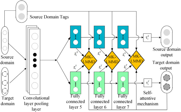
FIGURE 1. DSAN model based on self-attentive mechanism.

3 Transformer fault diagnosis based on magnetic field leakage characteristic

3.1 Load normalization of magnetic flux leakage

In this study, leakage magnetic field information is used to diagnose transformer faults. Because the load change of the transformer affects the current of the secondary winding and subsequently affects the amplitude and phase angle of the leakage magnetic field waveform, it will adversely affect the accuracy of fault classification. Previous papers have selected several different load conditions to analysis of leakage fields for different load conditions. In this paper, we propose a method based on real-time load normalization of the current on the first and second sides of the transformer.

To eliminate the influence of load changes on fault diagnosis, in this study, the amplitude and phase angle of the leakage magnetic field waveform are normalized using the currents at the primary and secondary windings of the transformer. The magnetic line of the leakage flux of the primary and secondary windings is closed along the nonferromagnetic material and is linear with the primary and secondary side currents (Gu, 2010). The resistive inductive load is the common load of a transformer. The change in load simultaneously affects the waveform of the leakage magnetic field amplitude and phase angle. The linear function between the leakage magnetic field and the response of the transformer primary and secondary side currents is as Eq. 13 (Gu, 2010):

${\dot{B}}_L=\dot{p}{\dot{I}}_1+\dot{q}{\dot{I}}_2(13)$

${\dot{B}}_L$ Indicates leakage magnetic field. $\dot{p},\dot{q}$ is constant coefficient, ${\dot{I}}_1,{\dot{I}}_2$ is the primary and secondary side current. When the transformer operates in any two different load states, the Eq. 14 shows:

$\begin{array}{l}{\dot{B}}_a^{*}=\dot{p}{\dot{I}}_{a1}^{*}+\dot{q}{\dot{I}}_{a2}^{*}\\ {\dot{B}}_b^{*}=\dot{p}{\dot{I}}_{b1}^{*}+\dot{q}{\dot{I}}_{b2}^{*}\end{array}(14)$

${\dot{B}}_a^{*},{\dot{B}}_b^{*}$ indicates the leakage magnetic field under two different loads. ${\dot{I}}_{a1}^{*},{\dot{I}}_{a2}^{*},{\dot{I}}_{b1}^{*},{\dot{I}}_{b2}^{*}$ is the primary and secondary side current under two different loads. When the transformer operates under the rated load, as shown in the Eq. 15:

${\dot{B}}_f^{*}=\dot{p}{\dot{I}}_{f1}^{*}+\dot{q}{\dot{I}}_{f2}^{*}(15)$

${\dot{B}}_f^{*}$ Indicates leakage magnetic field under the rated load. ${\dot{I}}_{f1}^{*},{\dot{I}}_{f2}^{*}$ is the primary and secondary side current under the rated load. Eq. 16 can be obtained from Eq. 14, 15:

${\dot{B}}_f^{*}=\left[\begin{array}{cc}{\dot{I}}_{f1}^{*}& {\dot{I}}_{f2}^{*}\end{array}\right]{\left[\begin{array}{cc}{\dot{I}}_{a1}^{*}& {\dot{I}}_{a2}^{*}\\ {\dot{I}}_{b1}^{*}& {\dot{I}}_{b2}^{*}\end{array}\right]}^{-1}\left[\begin{array}{c}{\dot{B}}_a^{*}\\ {\dot{B}}_b^{*}\end{array}\right](16)$

Eq. 16 shows that under any two load conditions, the leakage magnetic field intensity of any measuring point can be normalized to the rated load condition, which avoids the interference of load fluctuation on the fault classification.

3.2 Extraction of Lissajous figure feature quantity of magnetic field leakage

The transformer used in this experiment was a toroidal core transformer, which is widely used in electronic equipment with high technical requirements, and it primarily serves as a power transformer. From the perspective of straightening the iron core, the radial magnetic field leakage is equivalent to the axial direction of the core transformer, and the tangential direction is equivalent to the radial direction of the core transformer. This is called the radial direction and the tangential direction is called the axial direction. In this study, the primary and secondary-side windings of the A-phase Y/Y connection of the three-phase transformer are used as an example for testing.

When an early fault occurs in the transformer, it can be found by analyzing the waveform of the leakage magnetic field that the change in the leakage magnetic field at the end and central positions of the transformer is the most evident, and there are distinct differences in different fault types. To distinguish the different fault types of the winding, it is proposed set a measuring point at the two ends and central positions of the winding to measure the axial and radial leakage magnetic fields. The measurement point position of the transformer leakage magnetic field is illustrated in Figure 2.

FIGURE 2

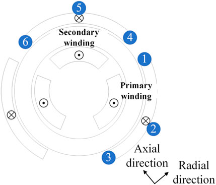
FIGURE 2. Schematic diagram of transformer measurement points.

Previous studies have only used the amplitude and phase angle of the leakage field at individual measurement points, but for transformer faults it is the internal leakage field balance that changes. The relationship of the leakage field between the measurement points is also important information. We propose a method that uses the Lissajous image of the leakage field signal to better integrate the information between these measurement points. The transformer leakage magnetic field waveform is a harmonic signal and the Lissajous figure is widely used in harmonic signal processing (Zhao et al., 2019). When the transformer fails, the symmetry of the magnetic field leakage at both ends of the winding changes. The Lissajous figure drawn by the leakage magnetic field waveform at measuring points 1, 3 and 4, 6 can reflect the change in the symmetry of the winding at the time. The leakage magnetic field in the middle of the fault winding changes; however, that of the non-fault winding remains unchanged. The Lissajous figure drawn by the leakage magnetic field waveform at 2, 5 measuring points can reflect this mutation. To make the fault characteristics more intuitive, this work deduces the length, swing angle, area, least square radius, and roundness of the long and short axes of the Lissajous figure as characteristic parameters that reflect the change in the leakage magnetic field amplitude and phase angle. Considering the leakage magnetic field waveform of 1, 3 measuring points as an example, the characteristic quantity of the leakage magnetic field is calculated. Assuming that the leakage magnetic field waveform of measuring points 1, 3 is as shown in Eq. 17:

$\{\begin{array}{c}{B}_1=M\cos \left(\omega t+{\psi }_1\right)\\ B_3=N\cos \left(\omega t+{\psi }_3\right)\end{array}(17)$

$M,N$ indicate the amplitude of the magnetic field leakage, and $\xi ={\psi }_1-{\psi }_3$ is defined as the phase angle difference between points 1, 3 measuring points. Solve the equation, we obtain the length of the long- and short-axis $a、b$ of the Lissajous figure, as follows Eq. 18:

$\begin{array}{l}{a}^2\mathrm{o}\mathrm{r}{b}^2=\\ \frac{\left(M^2+N^2\right)\mp \sqrt{{\left(M^2+N^2\right)}^2-4M^2{N}^2{\sin }^2\xi }}{2}\end{array}(18)$

According to the elliptic area formula, the area of the Lissajous figure is calculated using $\mathrm{S}=\pi ab$.

The coordinates are rotated to calculate the swing angle of the Lissajous figure as follows Eq. 19:

${\theta }_Q=\frac{1}{2}\arctan \frac{2MN\cos \xi }{N^2-M^2},N\ne M(19)$

It is evident from the above formulas that the long-short axis, area, and swing angle of the leakage magnetic field Lissajous figure are functions of the amplitude and phase difference of measuring points 1, 3, and the fault information of the leakage magnetic field represented by it is more abundant, which is conducive to improving the accuracy of classification.

Assuming that $u、v$ is divided into $m$ points of $u_i、v_i\left(i=\mathrm{1,2},\dots ,m\right)$ following sampling, then the center coordinate of the least square circle is ($u_0=\frac{2}{m}{\displaystyle \sum }_i^m{u}_i$; $v_0=\frac{2}{m}{\displaystyle \sum }_i^m{v}_i$). The radius of the least square circle of Lissajous figure is $r_0=\frac{1}{m}{\displaystyle \sum }_{i=1}^m\sqrt{\left(u_i^2+v_i^2\right)}$, and the distance between the first point and the least square center is as follows Eq. 20:

$r_i=\sqrt{{\left(u_i-u_0\right)}^2+{\left(v_i-v_0\right)}^2}(20)$

The circularity of the Lissajous graph is $e=\max \left(r_i\right)-\min \left(r_i\right)$.

The change in the least square radius of the Lissajous figure reflects the change in the amplitude of the leakage magnetic field waveform, and the change in the roundness reflects the change in the phase difference of the leakage magnetic field waveform. It can also be used as a characteristic quantity of the magnetic field leakage for transformer fault diagnosis.

3.3 Transformer early fault diagnosis process

First, the CNN classification model was constructed by offline learning the fault leakage magnetic field characteristics of the simulation transformer model. Second, the actual transformer fault is diagnosed by online measurement and extraction of the magnetic field leakage characteristics of the actual transformer. The early fault diagnosis process of the transformer is as follows.

3.3.1 Simulation model construction and actual transformer experimental platform construction

1) Measured actual transformer structure data and electrical parameters on the nameplate to establish a 1: 1 actual transformer simulation model.

2) Develop the actual transformer fault simulation and magnetic field leakage measurement platform.

3.3.2 Data generation

1) An actual transformer simulation model was used to simulate the possible faults in the transformer under different load conditions. The current on the primary and secondary windings of the transformer and the waveform data of the leakage magnetic field at each measuring point were recorded. The measured current data are normalized by the formula in Section 3.1, and the characteristic quantity of the magnetic field leakage is calculated. The gray image formed by the characteristic quantity of the magnetic field leakage is considered as the sample data ${\mathit{x}}_s$, and the label ${\mathit{y}}_s$ is added according to the fault type to generate the training sample ${\mathit{D}}_S$. Part of the data was randomly divided into training dataset ${\mathit{D}}_{\mathrm{t}\mathrm{r}\mathrm{a}\mathrm{i}\mathrm{n}}$, and another part of the data was randomly divided into validation dataset ${\mathit{D}}_{\mathrm{v}\mathrm{a}\mathrm{l}\mathrm{i}\mathrm{d}}$.

2) Normal operation, inter-turn short circuit, and winding deformation experiments of the actual transformer experimental platform were performed, and the data were recorded. The measured data from the actual transformer are used to constitute the test sample. ${\mathit{D}}_T$.

3.3.3 Network structure and acceleration algorithm

Because the input image is small, to fully extract its feature information, the kernel functions of the convolution and pooling layers in the CNN are both large. The momentum- updating stochastic gradient descent (SGD) acceleration algorithm was used to improve the network training speed. Offline model training was terminated when the error was less than the set value. The online detection model inherits the convolution layer parameters completed by offline training, and its full connection layer parameters are randomly initialized.

3.3.4 Parameter update and stop

1) The loss function of the offline CNN model is calculated according to the actual label data and label output predicted by the classifier and stops after the error reaches the set value.

2) The online model uses direct transfer learning. After calculating the transfer loss and classification loss by MK-LMMD regularization, the full connection layer parameters in the CNN model were retrained until the set number of training was reached.

3) Online model parameter updating refers to online model updating by re-labelling the monitored fault data following manual verification after each running period of online detection.

The overall flowchart of the transformer early fault diagnosis model based on CNN transfer learning is illustrated in Figure 3.

FIGURE 3

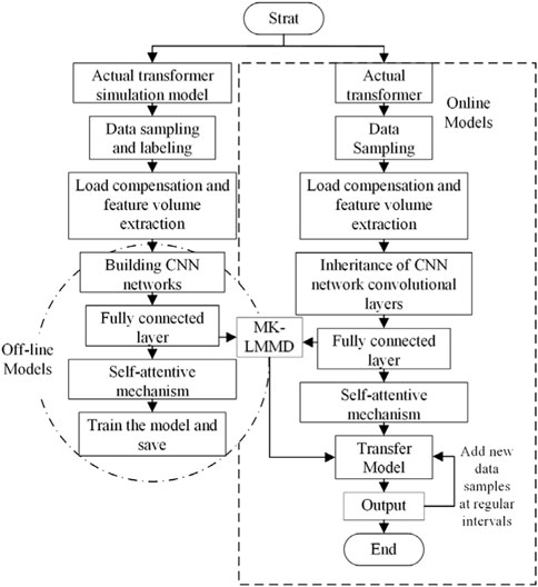
FIGURE 3. System operation flowchart.

FIGURE 4

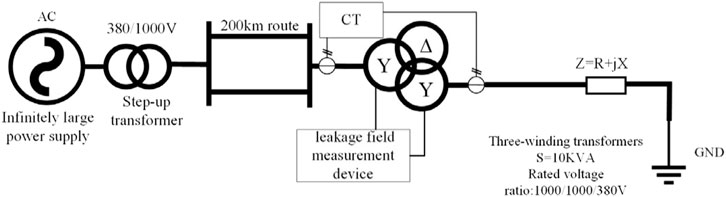
FIGURE 4. Transformer leakage magnetic field measurement.

4 Example analysis

4.1 The establishment of simulation model and actual transformer experimental platform

4.1.1 Transformer simulation model

The ANSYS MAXWELL software used in this study simulated an actual transformer. In the actual measurement, the sensor only measure the axial and radial leakage magnetic field waveforms in the transformer section. To reduce the generation time of the simulation data, only the two-dimensional (2D) section model of the ring core transformer is established. The solution area of the model was set according to the actual box size, and the primary and secondary windings were connected using a star connection. The 2D model of the transformer was set up, as shown in Supplementary Appendix B2, and the grid value was set according to the empirical value.

4.1.2 The construction of the actual transformer early fault experimental platform

A wiring diagram of the actual experimental platform system is shown in the Figure 4. Infinite power $E=380\mathrm{V}$, with no internal resistance, passes through the high-voltage bus via the boost transformer. The test transformer was a three-phase, three-winding transformer. Primary and secondary windings with a Y-shaped connection were used for the experiment. Secondary windings with angular connections were unloaded. The structural and electrical parameters of the transformer are listed in Supplementary Appendix A2. The rated load parameter is $Z_L=159.98+j1.35\Omega$. The load adjustment ranges were $Z_{\mathrm{L}\mathrm{m}\mathrm{i}\mathrm{n}}=107.89+j0.858\Omega$, $Z_{\mathrm{L}\mathrm{m}\mathrm{a}\mathrm{x}}=212.08+j2.02.\Omega$.

4.1.3 Transformer leakage magnetic field measurement platform

We developed a fiber optic leakage magnetic field sensor based on a magneto-optical crystal to collect the actual transformer magnetic field leakage waveform according to the Faraday magneto-optical effect. A sensor probe was installed on the transformer winding. The laser emitter emitted a light signal through the optical signal polarizer and Faraday rotator, and the other end detected the deflection angle of the optical signal through the optical signal receiver and converted it to leakage magnetic field intensity. A leakage magnetic field measurement platform was built on an actual transformer experimental platform, as displayed in Figure 5.

FIGURE 5

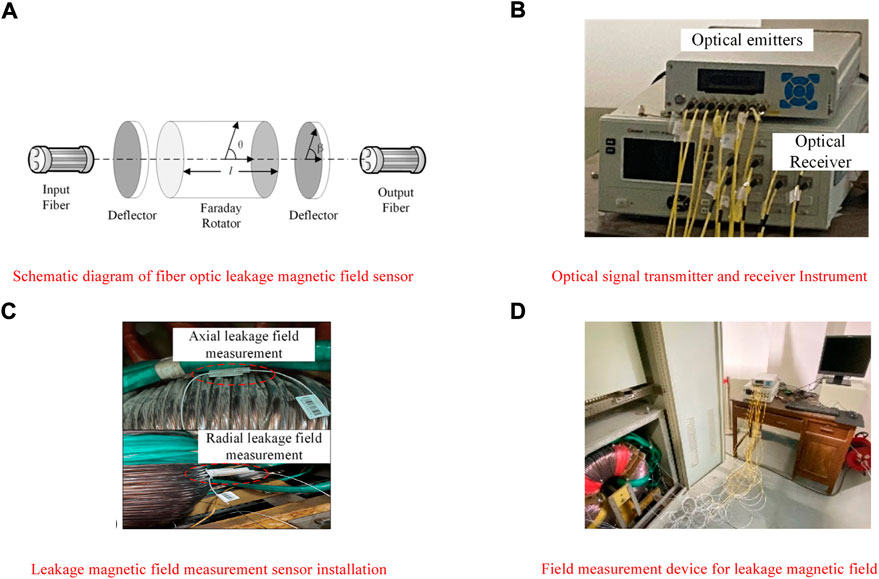
FIGURE 5. Transformer leakage magnetic field measurement device and installation schematic. (A) Schematic diagram of fiber optic leakage magnetic field sensor. (B) Optical signal transmitter and receiver Instrument. (C) Leakage magnetic field measurement sensor installation. (D) Field measurement device for leakage magnetic field.

4.2 Generation and processing of leakage magnetic field experimental data

4.2.1 Training sample generation

During the normal operation of the transformer, several groups of normal operation state data of the transformer were generated according to the different load values, and several groups of data were generated by changing the number of turns, the position, and the load of the primary and secondary side winding short circuits, respectively. The minimum number of short-circuit turns is two, and the maximum is 40 turns. In the simulation of the winding axial deformation fault, the axial deformation degree of the upper or double ends of the primary and secondary side windings were changed, the axial compression ratio ranged from 1% to 40%, and several groups of data were generated by changing the load. In the fault simulation of the radial deformation of the winding, the proportion of the radial deformation of the primary- and secondary-side windings changes from 3% to 25%. Different training data were generated according to different radial deformation ratios, the position of the radial deformation line cake, and the load. Each state type of the simulation model generated 125 groups of sample data and a total of 1,125 groups of training sample data.

4.2.2 Test sample generation

The test samples were generated by the actual transformer, and several groups of data for normal operation under different loads were generated by the actual transformer. In the inter-turn short-circuit test of the primary and secondary windings, the minimum is 6 turns and the maximum is 24 turns, and several groups of data were obtained under different loads. Winding deformation test on transformer to change the degree of axial and radial deformation of the primary and secondary windings to form training samples. Each state type generated 20 groups of sample data with 180 groups of test-data waveforms.

4.2.3 Comparison between simulation model and actual transformer normal operation and inter-turn short circuit

A sampling frequency of 1 kHz was used for all samples in this study. Except for the actual measured waveforms, the data were filtered. A comparison of the measured and simulated waveforms of the transformer leakage field is shown in Figure 6.

FIGURE 6

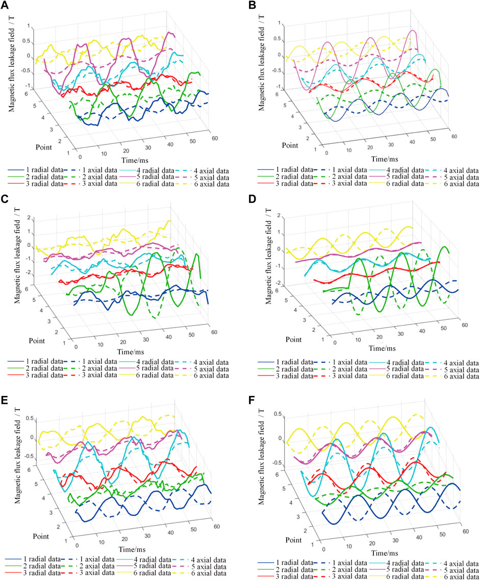
FIGURE 6. Measured waveform of transformer leakage magnetic field. (A) Measured waveform of normal Operation leakage magnetic field. (B) Simulation waveform of normal operation leakage magnetic field. (C) Measurement Waveform of Interturn Short Circuit leakage magnetic field. (D) Simulation waveform of interturn short circuit leakage magnetic field. (E) The Measured waveform of winding deformation leakage magnetic field. (F) Simulation waveform of winding deformation leakage magnetic field.

It can be observed from Figure 6, the amplitude and phase angle of the leakage field at our selected measurement points change to different degrees when the transformer is in normal condition and a fault occurs. We use the Lissajous curve proposed in Section 3.2 to extract the changes in the characteristic quantities at the time of the fault as input to the CNN and use artificial intelligence techniques to analyze the differences for transformer winding fault classification. Meanwhile, there is still a gap between the simulation waveform and the actual waveform difference. DSAN realizes domain adaptation by aligning its distribution difference and achieves the ability to diagnose actual transformer faults using simulation data.

4.2.4 Lissajous figure comparison before and after load normalization

The measured radial leakage magnetic fields at 1, 3 are plotted as Lissajous figures under the rated load, respectively, as shown in Figure 7A. It is evident that the Lissajous figures change with the change in load, which adversely affects the classification accuracy. Figure 7B illustrates the Lissajous figures of measuring points 1, 3 after load normalization. It is evident that after load normalization, the change of Lissajous figure caused by the change of transformer load is eliminated, and the characteristic quantity of leakage magnetic field is not affected by the load.

FIGURE 7

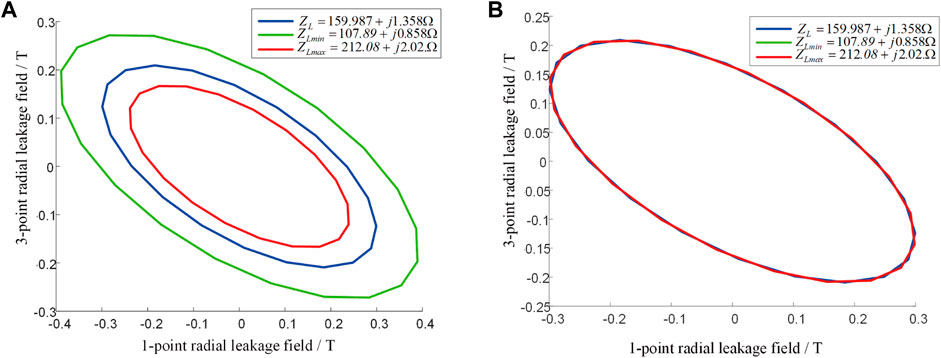
FIGURE 7. Lissajous figure before and after load normalization. (A) Before normalization. (B) After normalization.

4.2.5 Lissajous figure feature extraction and gray image generation

The characteristic quantity of the Lissajous figure formed by the leakage magnetic field was extracted, and the data were transformed into gray image data of 6 × 6. The gray image formed by the characteristic quantity of the transformer winding is shown in Supplementary Appendix B3, B4.

4.3 Example analysis

The transfer neural network prepared in this study is based on Python 3.6 version and Pytorch version 1.2.0. CPU training was then performed. The CPU of the computer was an AMD Ryzen 7 4800 H, and the main frequency was 2.90 GHz. A batch of 10 sets of data, initial learning rate 0.4, training 100 Epohs, MK-LMMD regularizer penalty factor initial value $\lambda =1$. The transformer states in this paper are divided into normal operation, winding deformation and inter-turn short circuit. The inter-turn short circuit is subdivided into primary winding inter-turn short circuit and secondary winding inter-turn short circuit. The winding deformation is subdivided into nine states, namely, the axial deformation at the upper end of primary and secondary side winding, the axial deformation at the two ends of primary and secondary side winding, and the radial deformation of primary and secondary side winding. The operation state of the transformer is coded as shown in Supplementary Appendix A3.

4.3.1 Load normalization and simulation sample number experiments

To test the influence of load balances and the number of simulation samples participating in training on transformer fault diagnosis, we also generated gray images for training and testing the data without load normalization. Simultaneously, to detect the influence of the number of simulation samples on the detection effect, different numbers of simulation samples were selected for offline training. To ensure that the data of the offline training test set were unchanged, a certain number of simulation samples were randomly selected as the training set, and samples without and after load normalization were tested. The accuracy results are presented in Figure 8.

FIGURE 8

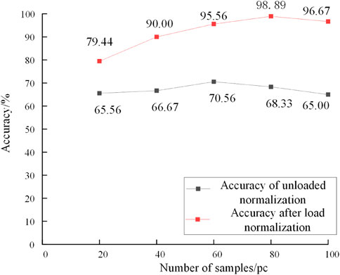
FIGURE 8. Effect of different number of simulation sample data and load normalized on detection accuracy.

It is evident from the above diagram that load normalization has a significant impact on overall accuracy. Load normalization can significantly improve the transformer detection accuracy. Compared with the unnormalized load data, the highest accuracy increased by 28.33%. Simultaneously, the number of training sets also affects the detection accuracy. Increasing the number of simulation samples did not always improve the accuracy of the test. When the number of simulation samples is too large, the model focuses on the detection of simulation samples, which reduces the accuracy of the actual transformer detection. When the number of simulation samples was 80 in each state, the accuracy was the highest, and the accuracy did not increase again when the number of training samples increased.

4.3.2 Experiment on the quantity of characteristic quantities of magnetic field leakages

To test the influence of the leakage magnetic field characteristics on the accuracy of the transformer fault diagnosis, different quantities of characteristics were selected for training and testing, and the accuracy of classification was compared. For the experimental group without feature parameters, we directly used the amplitude and phase angle data of the six measuring points to load balance and convert them into gray images for testing. Recall rate $R_m$, stability comprehensive index ${\mathrm{F}}_1$, and accuracy $A_c$ were used as evaluation indexes. Table 1 presents the results.

TABLE 1

TABLE 1. Effect of different characteristic quantity on detection accuracy.

It can be observed from Table 1 that the method of using the characteristic quantity has a positive effect on enhancing the accuracy of transformer diagnosis. Compared with the method of using only the amplitude and phase angle of the leakage magnetic field to diagnose faults, the accuracy of this method was improved by 6.67%.

4.3.3 MK-LMMD regularizer layer experiment

The data of the 80 simulation groups for each fault state were used as training samples, and the measured waveform was used as the test sample. To test the effect of adding different numbers of MK-LMMD regularizers on the test results, the training results of adding MK-LMMD regularizers in the last layer, last two layers, and three layers of the full connection layer were tested and compared with the results of the CNN classification model without transfer learning. The results are as follows. Table 2 presents that the accuracy curve of the classification model with different numbers of MK-LMMD regularizer layers increases with the number of iterations, as shown in Figure 9.

TABLE 2

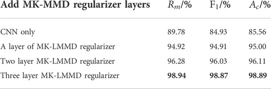
TABLE 2. Effect of different regularizer layers on accuracy.

FIGURE 9

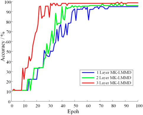
FIGURE 9. Transfer learning training correct rate curve.

Table 2 indicates that the difference between the simulation data and the actual transformer data cannot be overcome when the non-transfer CNN fault classification model is directly used for actual transformer detection, resulting in unsatisfactory accuracy of the actual transformer fault classification. As shown in Figure 9, the classification model with three-layer MK-LMMD regularization has the highest accuracy and fastest convergence rate, which is 13.33% higher than that with only CNN.

The transformer fault features extracted from the model with MK-LMMD regularizers of different layers were reduced to 2D visualization by T-SNE, as shown in Figure 10.

FIGURE 10

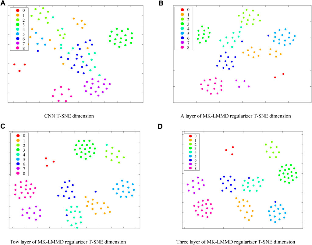
FIGURE 10. Comparison of T-SNE scatter plots under different training models. (A) CNN T-SNE dimension. (B) A layer of MK-LMMD regularizer T-SNE dimension. (C) Tow layer of MK-LMMD regularizer T-SNE dimension. (D) Three layer of MK-LMMD regularizer T-SNE dimension.

In high-dimensional spatial data, the points with closer distances remain close when they are projected to 2D by T-SNE dimension reduction. The farther the distance of each cluster, the greater the difference and the better the classification effect. The results in Figure 10 reveal that the transfer learning model using three-layer MK-LMMD regularization has a better discrimination for different fault types of the actual transformer, indicating that increasing the adaptability of the high-order feature layer can effectively improve the transfer effect.

4.3.4 Self-attention mechanism deep subdomain adaptive network experiment

To verify the effect of the DSAN network with the self-attention mechanism, the data from 80 simulation groups for each fault state were used as training samples, and the measured waveform was used as the test sample. The error iteration curve obtained using training is illustrated in Figure 11.

FIGURE 11

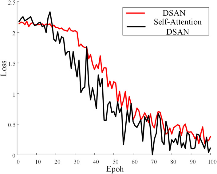
FIGURE 11. DSAN error curve of self-attentive mechanism.

Figure 11 shows that in the training process without giving training samples self-attention weights, some samples deviate too much from the test sample, resulting in large transfer error of MK-LMMD regularization, resulting in oscillation of error curve. The self-attention DSAN proposed in this paper can speed up the network training speed, reduce the error level, has good stability and reduce the training loss.

4.4 Comparative experiments with other transfer networks

To compare the proposed method with other transfer neural networks, the existing DAN transfer learning (Long and Wang, 2015), CORAL transfer learning (Sun and Saenko, 2016), GAN transfer learning (Hu et al., 2021), and traditional DSAN models are used for comparison (Zhu et al., 2021). In the experiments, the data of 80 simulation groups for each fault state were used as the simulation samples. The test results for the 20 groups of experimental samples in each group are listed in Table 3. The classification of the test samples is depicted in Figure 12. In Figure 12, the black solid line represents the true value of the fault type and the red circle represents the diagnostic value of the model for the fault. When the red circle coincides with the black line, it indicates that the diagnosis is correct; otherwise, the diagnosis is incorrect.

TABLE 3

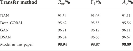
TABLE 3. Identification accuracy of different transfer methods in case of transformer faults.

FIGURE 12

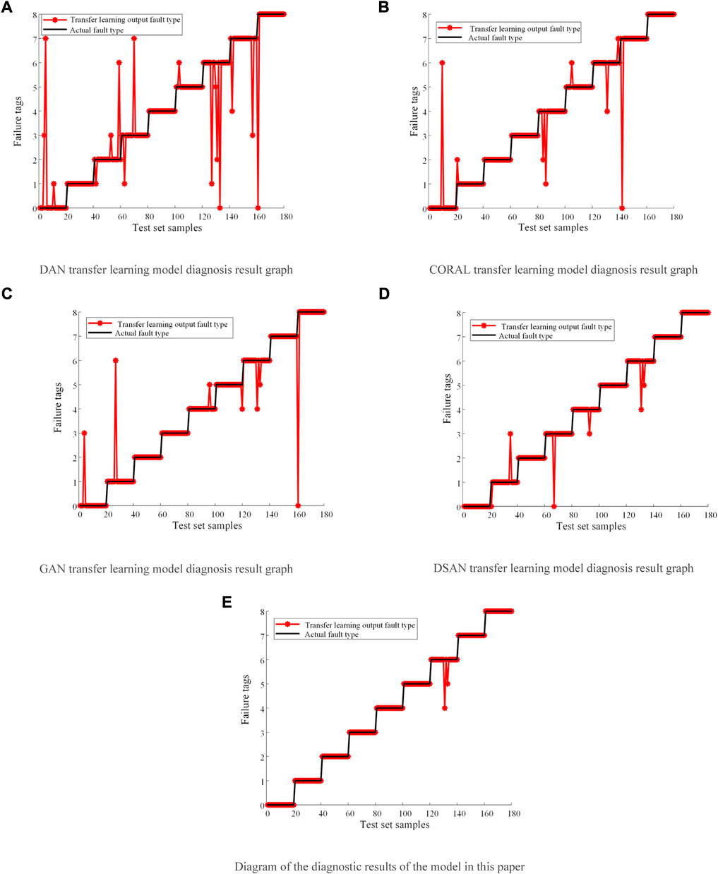
FIGURE 12. Comparison of diagnostic results of four different transfer models. (A) DAN transfer learning model diagnosis result graph. (B) CORAL transfer learning model diagnosis result graph. (C) GAN transfer learning model diagnosis result graph. (D) DSAN transfer learning model diagnosis result graph. (E) Diagram of the diagnostic results of the model in this paper.

Figure 12 illustrates that the method used in this study has the best classification effect. In addition to the misjudgment of the upper end winding deformation of the secondary side, the classification effect of the fault is superior. Compared with the other three transfer models, the MK-LMMD regularization and self-attention mechanism used in the proposed transfer model effectively reduced the distribution distance between the simulated transformer data and the actual transformer data, and realized the transfer from the simulated transformer to the actual transformer with high accuracy.

5 Conclusion

This paper eliminates the effect of transformer load variations on leakage field measurements by negative normalization and improves the utilization rate of the leakage magnetic field information. Meanwhile, transfer learning to reduce the difference between the simulation model and the actual transformer data and realizes the fault classification model trained by the simulation data to early diagnosis of actual transformer faults. The influence of load change in transformer leakage magnetic field detection is eliminated, and the characteristic quantity of the leakage magnetic field is extracted to diagnose transformer faults, which improves the utilization rate of the leakage magnetic field information. The accuracy of the method proposed in this paper reaches 98.89%, which is suitable for detecting and diagnosing the internal faults of transformer windings promptly via real-time acquisition of transformer faults and provides a reference for reasonable periodic shutdown maintenance of transformers. However, only one structure of transformer transfer learning ability is studied in this paper, for other structures of transformer simulation and transfer learning between actual transformers and mutual transfer between the different structure of transformers is our next research direction.

Data availability statement

The original contributions presented in the study are included in the article/Supplementary Material, further inquiries can be directed to the corresponding author.

Author contributions

The XD wrote the original draft. ZZ, KY, and HZ provided the supervision, review, and editing of the draft. All authors contributed to theatrical and approved the submitted version.

Funding

Funded by the National Nature Fund (51777119).

Conflict of interest

The authors declare that the research was conducted in the absence of any commercial or financial relationships that could be construed as a potential conflict of interest.

Publisher’s note

All claims expressed in this article are solely those of the authors and do not necessarily represent those of their affiliated organizations, or those of the publisher, the editors and the reviewers. Any product that may be evaluated in this article, or claim that may be made by its manufacturer, is not guaranteed or endorsed by the publisher.

Supplementary material

The Supplementary Material for this article can be found online at: https://www.frontiersin.org/articles/10.3389/fenrg.2022.1058378/full#supplementary-material

References

Alshehawy, A. M., Mansour, D. E. A., Ghali, M., Lehtonen, M., and Darwish, M. M. F. (2021). Photoluminescence spectroscopy measurements for effective condition assessment of transformer insulating oil. Processes 9 (5), 732. doi:10.3390/pr9050732

CrossRef Full Text | Google Scholar

Bo, Z., Xza, B., Zza, B., and Wu, Q. (2021). Deep multi-scale separable convolutional network with triple attention mechanism: A novel multi-task domain adaptation method for intelligent fault diagnosis. Expert Syst. Appl. 2021, 115087. doi:10.1016/j.eswa.2021.115087

CrossRef Full Text | Google Scholar

Cabanas, M. F., Melero, M. G., Pedrayes, F., Rojas, C. H., Orcajo, G. A., Cano, J. M., et al. (2007). A new online method based on leakage flux analysis for the early detection and location of insulating failures in power transformers: Application to remote condition monitoring. IEEE Trans. Power Deliv. 22 (3), 1591–1602. doi:10.1109/TPWRD.2006.881620

CrossRef Full Text | Google Scholar

Chen, Y. M., Liang, J., and Zhang, J. W. (2019). Method of online status monitoring for windings of three-winding transformer based on improved parameter identification. High. Volt. Eng. 45 (5), 1567–1575. doi:10.13336/j.1003-6520.hve.20190430029

CrossRef Full Text | Google Scholar

Deng, X. l., Xiong, X. F., and Gao, L. (2014). On line monitoring method of transformer winding deformation based on parameter identification CSEE. Proc.34 (28), 4950–4958. doi:10.13334/j.0258-8013.pcsee.2014.28.023

CrossRef Full Text | Google Scholar

Elsis, M., Minh, Q. T., Karar, M., Diaa-Eldin, A. M., Matti, L., and Darwish, M. M. F. (2022). Effective IoT-based deep learning platform for online fault diagnosis of power transformers against cyberattacks and data uncertainties. Meas. (. Mahwah. N. J). 2022, 110686. doi:10.1016/j.measurement.2021.110686

CrossRef Full Text | Google Scholar

Emara, M. M., Peppas, G. D., and Gonos, I. F. (2021). Two graphical shapes based on DGA for power transformer fault types discrimination. IEEE Trans. Dielectr. Electr. Insul. 28 (3), 981–987. doi:10.1109/TDEI.2021.009415

CrossRef Full Text | Google Scholar

Gao, J., and He, J. J. (2010). Application of quantum genetic ANNs in transformer dissolved gas-in-oil analysis. Proc. CSEE 30 (30), 121–127. doi:10.13334/j.0258-8013.pcsee.2010.30.020

CrossRef Full Text | Google Scholar

Ghifary, M., Kleijn, W. B., and Zhang, M. (2014). “Domain adaptive neural networks for object recognition,” in Pacific rim international conference on artificial intelligence (Cham: Springer), 898–904. doi:10.1007/978-3-319-13560-1_76

CrossRef Full Text | Google Scholar

Gu, C. L. (2010). Electrical engineering. Wuhan: Huazhong University of Science and Technology.

Google Scholar

Haghjoo, F., Mostafaei, M., and Mohammadi, H. (2017). A new leakage flux-based technique for turn-to-turn fault protection and faulty region identification in transformers. IEEE Trans. Power Deliv. 33, 671–679. doi:10.1109/TPWRD.2017.2688419

CrossRef Full Text | Google Scholar

Hang, W., and Butler, K. L. (2002). Modeling transformers with internal incipient faults. IEEE Trans. Power Deliv. 17 (2), 500–509. doi:10.1109/61.997926

CrossRef Full Text | Google Scholar

Hu, X., Zhang, H., Ma, D., and Wang, R. (2021). A tnGAN-based leak detection method for pipeline network considering incomplete sensor data. IEEE Trans. Instrum. Meas. 70, 1–10. doi:10.1109/TIM.2020.3045843

PubMed Abstract | CrossRef Full Text | Google Scholar

Jang, E., Gu, S. S., and Poole, B. (2017). Categorical reparameterization with gumbel-softmax. Available at: http//:ArXiv.org/abs/1611.01144. doi:10.48550/arXiv.1611.01144

CrossRef Full Text | Google Scholar

Lecun, Y., Bottou, L., Bengio, Y., and Haffner, P. (1998). Gradient-based learning applied to document recognition. Proc. IEEE 86 (11), 2278–2324. doi:10.1109/5.726791

CrossRef Full Text | Google Scholar

Li, H., Huang, Z. Y., and Tian, Y. (2022). Research on transformer fault diagnosis method based on deep neural network. Transformer 59 (04), 35–40. doi:10.19487/j.cnki.1001-8425.2022.04.014

CrossRef Full Text | Google Scholar

Liu, N., Liang, G. D., Wang, L. F., Gao, W. S., and Tan, K. X. (2003). Construction and analysis of fault tree for large-scalepower transformer. Electr. Power 36 (11), 33–36. doi:10.13336/j.1003-6520.hve.2003.02.002

CrossRef Full Text | Google Scholar

Long, M., and Wang, J. (2015). “Learning transferable features with deep adaptation networks,” in International conference on machine learning. PMLR 2015, 97–105. doi:10.1109/TPAMI.2018.2868685

CrossRef Full Text | Google Scholar

Naseri, F., Kazemi, Z., Arefi, M. M., and Farjah, E. (2018). Fast discrimination of transformer magnetizing current from internal faults: An extended kalman filter-based approach. IEEE Trans. Power Deliv. 33 (1), 110–118. doi:10.1109/TPWRD.2017.2695568

CrossRef Full Text | Google Scholar

Pan, C., Shi, W. X., and Meng, T. (2020). Study on electromagnetic characteristics of interturn short circuit of single-phase transformer. High. Volt. Eng. 46 (05), 1839–1856. doi:10.13336/j.1003-6520.hve.20200515040

CrossRef Full Text | Google Scholar

Shamlou, A., Feyzi, M. R., and Behjat, V. (2021). Winding deformation classification in a power transformer based on the time-frequency image of frequency response analysis using Hilbert-Huang transform and evidence theory. Int. J. Electr. Power & Energy Syst. 129 (5), 106854. doi:10.1016/j.ijepes.2021.106854

CrossRef Full Text | Google Scholar

Sun, B., and Saenko, K. (2016). Deep CORAL: Correlation alignment for deep domain adaptation. Berlin, Germany: Springer International Publishing.

Google Scholar

Wang, G., Giannakis, G. B., and Chen, J. (2019). Learning ReLU networks on linearly separable data: Algorithm, optimality, and generalization. IEEE Trans. Signal Process. 67 (9), 2357–2370. doi:10.1109/TSP.2019.2904921

CrossRef Full Text | Google Scholar

Wang, K., and Zeng, J. L. (2021). Simulation study of leakage field of power transformer under different operation modes based on field-path coupling. J. Harbin Inst. Technol. 26 (04), 28–37. doi:10.15938/j.jhust.2021.04.005

CrossRef Full Text | Google Scholar

Wang, X., and Han, T. (2021). Transformer fault diagnosis based on Bayesian optimized random forest. Electr. Meas. Instrum. 58 (6), 167–173.

Google Scholar

Wu, Z. H ., Zhou, M. B., Lin, Z. H., Chen, X. J., and Huang, Y. H. (2021). Improved genetic algorithm and XGBoost classifier for power transformer fault diagnosis. Front. Energy Res. 2021, 9. doi:10.3389/fenrg.2021.745744

CrossRef Full Text | Google Scholar

Zhang, B. Q., Xian, R., and Yu, Y. (2021). Analysis of physical characteristics of power transformer windings UnderInter-turn short circuit fault. High. Volt. Eng. 47 (06), 2177–2185. doi:10.13336/j.1003-6520.hve.20201178

CrossRef Full Text | Google Scholar

Zhang, J. C. (2019). Analysis of transformer winding leakage field and short-circuit electromotive force. Shenyang, China: Shenyang University of Technology.

Google Scholar

Zhao, X., Yao, C., Zhou, Z., Li, C., Abu-Siada, A., Zhu, T., et al. (2019). Experimental evaluation of transformer internal fault detection based on V–I characteristics. IEEE Trans. Ind. Electron. 67, 4108–4119. doi:10.1109/TIE.2019.2917368

CrossRef Full Text | Google Scholar

Zhou, Y. C., and Wang, X. (2017). The on-line monitoring method of transformer winding deformation based on magnetic field measurement. Electr. Meas. Instrum. 54 (17), 58–63.

Google Scholar

Zhu, Y. C., Zhuang, F. Z., Wang, J. D., Ke, G., Chen, J., Bian, J., et al. (2021). Deep subdomain adaptation network for image classification. IEEE Trans. Neural Netw. Learn. Syst. 32 (4), 1713–1722. doi:10.1109/TNNLS.2020.2988928

PubMed Abstract | CrossRef Full Text | Google Scholar