
94% of researchers rate our articles as excellent or good
Learn more about the work of our research integrity team to safeguard the quality of each article we publish.
Find out more
ORIGINAL RESEARCH article
Front. Energy Res., 21 October 2022
Sec. Solar Energy
Volume 10 - 2022 | https://doi.org/10.3389/fenrg.2022.1029449
This article is part of the Research TopicSolar Radiation and Photovoltaic System ForecastingView all 5 articles
 Ankur Kumar Gupta1,2*
 Rishi Kumar Singh1
The work of forecasting solar power is becoming more crucial with directives to regulate the quality of the power and increase the system’s reliability as photovoltaic (PV) sites are being integrated into the architecture of power systems at an increasing rate. This study proposes a metaheuristic model for short-term photovoltaic power forecasting that includes shuffled frog leaping algorithm (SFLA), principal component analysis (PCA), and generalized regression neural network (GRNN). In this model, GRNN is implemented to analyze the input parameters after the dimension reduction process, and its parameters get optimized with the help of the SFLA, which has the advantage of fast convergence speed as well as searching ability, whereas PCA techniques are implemented to diminish the dimension of meteorological conditions. This hybrid model achieves day-ahead short-term forecasting, as shown in an experimental case of a Bhadla Solar Park installed in Gujarat, India. The accuracy of the proposed model obtained a mean absolute error (nMAE) of 2.3325, and a root mean square error (RMSE) of 129.425. Similarly, the error in forecasting obtained by the proposed method results in nMAE = 2.977 and RMSE = 160.92. The output results obtained surpassed all other hybrid models used for comparison in this study.
Electricity, among various sources of energy, has a significant part in today’s world. Energy consumption is predicted to rise as the world becomes more globalized and modernized. Fossil fuels such as coal, gas, and diesel were various options for generating electricity in the past. Despite the fact that these energy sources are capable of meeting the electrical demand, their widespread use has resulted in the catastrophic depletion of fossil fuels and environmental issues (Lara Fanego et al., 2012). Crude oil, coal, and oil and gas, are expected to last 35, 107, and 37 years, respectively (Raza et al., 2016). The use of coal-fired power plants to generate power has led to enormous pollution in terms of CO2 emissions, which leads to global warming. In light of these realities, various alternative sources of energy used to meet energy needs have been intensively investigated. Renewable energy sources (RESs) have piqued global attention as such alternatives. Renewable power generation grew by 7% in 2020, of which 60% of the contribution was made by wind and solar PV technologies. Renewable sources accounted for about 29% of global electricity generation for 2020. Figure 1 shows the current scenario of the contribution made by various renewable energy sources to power generation in the world. The decline in energy demands induced by COVID-19 halted business growth and transit; on the other hand, it also proved to be a major contributor to this record. To achieve net zero emissions by 2050, more than 60% of generation by 2030 should be done by renewable power, which will require a dramatic increase in their installations. Though the net zero emission levels are to be achieved by 2050, there is a development in the yearly generation that averages 24% points throughout 2020 and 2030, culminating in 645 GW of net capacity additions in 2030 (IEA, 2018).
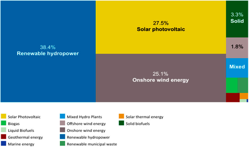
FIGURE 1. Contribution by renewable energy sources in total power generation.
PV technologies are gaining popularity nowadays due to their various features such as zero emission, zero fuel consumption, low operating and maintenance costs, no moving systems, silence, and ease of integrating with a grid. The solar photovoltaic output has increased by 157 TWh (24.2%), reaching 928 TWh in 2021 (IEA, 2018). It grew at the second-fastest rate among other green technologies in 2021, after wind, although it is ahead of hydropower. Photovoltaic electricity production attained an all-time high of 140 GW due to impending regulatory constraints in China, the United States, and Vietnam. In most regions around the world, rooftop solar has now become the best option for power generation, which is projected to spur expansion in the coming years. Figure 2 shows the installed solar capacity in countries like China, India, Spain, Brazil, Mexico, and Chile during the years 1996–2020. Figure 2 shows the PV installed capacity of different countries year-wise. PV power generation is influenced by certain factors which include weather conditions, pressure and velocity of the wind, ambient temperature, humidity, and solar irradiance (Kroposki, 2017). The power generated through PV systems is affected by climatological changes.
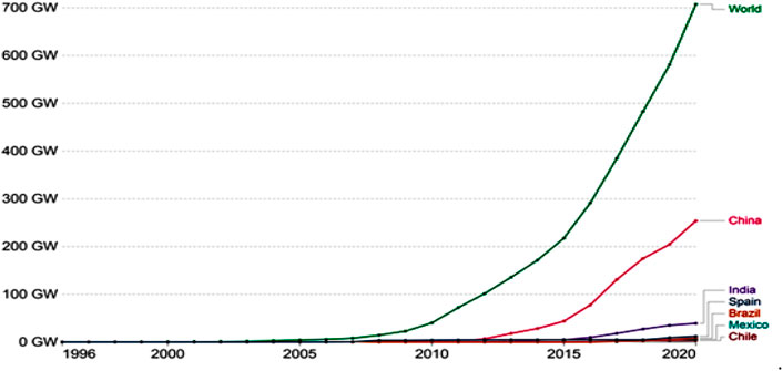
FIGURE 2. Installed solar PV capacity year wise (1996–2020).
The power system’s reliability, stability, and planning are all disrupted by a sudden change in solar power output. To avoid such situations, precise and exact photovoltaic output forecasting is needed, which also assures the power performance of the model, stability, and quality. It has the potential to lessen the grid’s impact on power uncertainty (Paulescu et al., 2013). Figure 3 shows the percentage contribution of PV systems in electrical power generation in different countries in a particular year ranging from 2017 to 2021. In a study by Yang et al. (2014), an artificial neural network (ANN) was implemented for PV forecasting for a one-day-ahead term. Another approach for PV power forecasting using back propagation ANN was constructed on the basis of seasonal weather classification considering 24 h (Eseye et al., 2018), where AI data are considered to be an input parameter. Similarly, weather forecasting reports are employed in PV power forecasting using ANN as was done by Asrari et al. (2017). The control of local supply and demand is shown by a confidence interval result. The results showed a good match between the target and the neighboring area using real-time correlation data. To improve the prediction accuracy as well as computational efficiency, a dendritic neuron network-based model for forecasting PV power was developed by Kushwaha and Pindoriya (2019). A wavelet transformation is introduced to extract frequencies of input data results to achieve diversity and accuracy in PV power forecasted results; a neural network ensemble scheme is proposed by Raza et al. (2019). In this scheme, five different feed-forward neural networks (FNNs) are trained using the particle swarm optimization (PSO) technique. The results are combined using Trim aggregation. An innovative prediction technique using an RNN model with echo state networks was introduced by Rosato et al. (2019) for forecasting the amount of generated PV power.
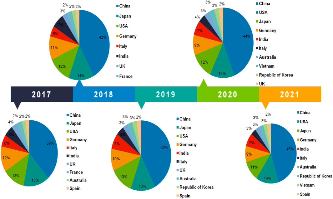
FIGURE 3. Milestone for solar installed capacity by different countries year wise.
Although solar irradiance is tightly correlated with PV output, several complicated meteorological conditions, such as temperature, humidity, precipitation, and others, also have an impact (Ramakrishna et al., 2019). Artificial intelligence techniques work on the principle of the central intelligence nervous system, which can be used to identify the patterns of recognition as well as machine learning. Prediction of PV power output on an hourly basis done using hybrid models based on similarly customized different algorithms are proposed by Zhang et al. (2020). A short-term forecast of power obtained from the residential PV system using SVM based on a genetic algorithm (GA) is introduced in Theocharides et al. (2020), where historical data are classified using an SVM classifier and further optimized using GA. An improvement in the regression coefficient of the PV model used for ultra-short-term PV power forecasting is seen in the study by Pan et al. (2020), where SVM is developed by preprocessing the data and optimizing its parameters using ant colony optimization. The wavelet transformation (WT), SVM, and PSO are combined for PV power forecasting for a one-day-ahead term in a real microgrid PV system. SVM maps meteorological variables from numerical weather prediction (NWP), and ill-behaved data which are affected by wavelets. An advanced statistical method self-organized map (SOM) proposed by Chen et al. (2011) is trained for classifying the data obtained by online meteorological services for a 24-hour-ahead local weather type. Similarly, a hybrid model is proposed by Zhu et al. (2016) where historically collected data are classified using SOM with learning vector quantization (LVQ); SVR also trained the datasets, and finally, the accurate model for PV power 1-day ahead hourly forecasting is selected with the help of fuzzy inference.
A hybrid model was proposed for short-term day-ahead PV power forecasting by Ge et al. (2020). The model achieves a high precision in forecasting under strong uncertainties. The hybrid model used seasonal auto-regressive integrated moving average (SARIMA) and ANN model for short-term forecasting and computation of PV power using the least squares method. Researchers in a study by Lin et al. (2018) constructed a framework for PV forecasting which has several stages. They are data quality stage, data-driven ANN model development, assessment of weather clustering (k-means clustering), linear regressive correction technique for optimizing output, and evaluation of the accuracy of the final performance. Similarly, for short-term forecasting for generated PV power, a hybrid model is developed using the improved technique of Grey relational analysis (GRA), K-means clustering, and Elman neural network (ENN) by Zhou et al. (2020). A novel hybrid method based on maximum overlap discrete wavelet transform is introduced by Haque et al. (2013), where SARIMA and random vector functional link (RVFL) neural network was hybridized for PV power forecasting. A fuzzy clustering of atmospheric turbidity, solar irradiance, and relative humidity using improved fuzzy c-means clustering (IFCM) technique was done by Jinpeng et al. (2022). Radial basis function (RBF) and genetic algorithm programming system (GAPS) were proposed for improving prediction accuracy.
The correlation between uncertainty in PV power and its consumption by thermostatically loading is described by Ramakrishna et al. (2019), where the first model developed uses a regime-switching process to incorporate the variations in PV power during cloudy, sunny, and partly cloudy conditions. A Volterra model of second order shows the relationship between temperature and solar power. The combination of these two models leverages the joint probability of PV power forecasting. A probabilistic ensemble method (PEM) where solar irradiation forecast is used to cluster the data based on solar irradiance is proposed for PV power forecasting by Pretto et al. (2022), where PEM is validated by a real-case study that uses data for 3 years. The RMSE metric was improved in this case compared to the mean value ensemble. The proposed model was executed for ultra-short-term prediction (Mei et al., 2018), where the model was divided into two sub-models which deal with offline forecasting and online forecasting. A regression sub-model of PV output and a weather classification model are established using an offline module, whereas real-time data are used by the online module to identify weather types. In this study, a short-term day-ahead PV power forecasting model is proposed using PCA-SFLA-GRNN. GRNN, a part of ANN techniques, has strong non-linear mapping capability, error tolerance, and robustness. Consequently, in this research, the Shuffled Frog Leaping Algorithm (SFLA) technique automatically determines the different parameter values of the GRNN model. This work suggests a new hybrid model to forecast PV output using a two-step method of SFLA and GRNN, as shown in Figure 4. This proposed model is based on the aforementioned literature analysis.

FIGURE 4. Flow diagram of forecasting using PCA-SFLA-GRNN.
The key aims of this research, with an emphasis on short-term PV output predictions for the day ahead, are:
1) To mitigate the dimension of the input data and avoid overfitting, minimizing the co-linearity of input data. Therefore, the PCA techniques are implemented to diminish the dimension of meteorological conditions.
2) The proposed GRNN-SFLA model for short-term PV forecasting over the next day. Where GRNN is implemented to fit the complex non-linear relationship between the PV input and output features, the GRNN technique is optimized using SFLA. For validation, the case study has been proposed for accuracy and robustness.
The energy used for PV output is entirely derived from solar irradiance. Thus, it can be said that the PV output is directly impacted by solar irradiance. The output of a PV plant may also be affected by meteorological factors like ambient temperature, wind speed, humidity, and atmospheric pressure. This may lead to a burden during the training of datasets, and it also affects the learning speed. However, it will minimize the sensitivity of forecasting models. So, we have to assume that there are x number of samples and each sample has y variables so that we can create an x * y data matrix. The dataset of Bhadla Solar Park is considered here for research purposes. It is located in the Jodhpur district of Rajasthan, India, on the coordinates of 27.5396685°N and 71.9152528°E with an area of 5,700°ha. The solar park consists of flat mounted PV panels. The temperature of this area is between 46°C and 48°C. The total installed capacity of the plant is 2,245 MW. A satellite view of Bhadla Solar Park is shown in Figure 5. The flowchart of PCA used for diminishing the dimensions of meteorological conditions is shown in Figure 6.
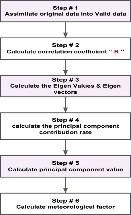
FIGURE 5. Stepwise process of PCA.
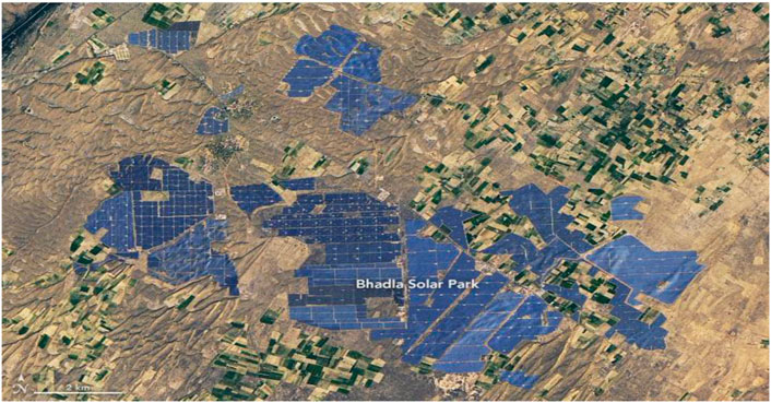
FIGURE 6. Satellite view of solar PV sites installed in Gujarat (Site 1 and 2 Bhadla Solar Park, Gujarat, India).
SFLA is a conceptually based algorithm that mimics the onomatopoeic progression of a community of hungry frogs. This algorithm’s design is conceptualized as a group of frogs that resides in a morass comprising several stone blocks. The primary goal of all the amphibians is to search for a rock having more quantity of food as compared to the other rocks. To discover and reach that stage, the frogs converse with one another while looking for ways to improve one another’s positions (memes) in the swamp. SFLA is built on the strategic planning of these frogs. To replicate this communications strategy and enforce SFLA, two different logics are blended. These logics are “deterministic” strategies and “random” strategies. The deterministic method is associated with the frogs’ local improved performance in the swamp. As a consequence, they can only interact with frogs from the same meiotic division. This model comprises three primary operators which are described below:
1) Classification stage: The primary objective is to acquire new categories of frogs. These frog categories are sequences of parallel frog cultures going to be used in the next step for local communication. The frogs are arranged first on the basis of their fitness for this intent. The frog with the best fitness must be placed in first class. This frog is termed the best frog in the swamp and the first member of the sorted set. Similarly, the second frog will be included in the second class. The nth frog will be included in the nth class, and a further (n+1)th frog will be introduced in the first class, and so on.
2) Local search stage: During this phase, the operator in each class allows the worst frog to interact with the best frog in an attempt to transform its leaping move and guidance in terms of improving its position. This procedure will be repeated several times for every SFLA simulation iterative process (epochs). As a result, the current worst frog of the class at the related epoch communicates with the recent best frog in that epoch to get nearer to the best rock in the swamp. (1) and (2) are the formulae that clarify the principle of local search:
Here, we consider indicate the position/locations of the fittest frog, the current default frog, and the generated frog, respectively. X and
The
3) Shuffling process stage: Each iteration ends after the epochs of local search have been completed for different classes. In this phase, all the frogs are combined, forming a unified population having zero bias. In the SFLA iterative process, these three agents are reiterated again and again until the stopping condition is reached (Ge et al., 2020). This stage must go into considerable detail about the SFLA idea as well as its execution.
GRNN constitutes four layers. The layers are the input layer, the pattern layer, the summation layer, and the output layer. Y represents the corresponding incoming and outgoing vectors, that is, Y = [
The count of neurons in each layer is equal to the input dimension of the training samples, and each neuron sends input data directly to the pattern layer. The count of neurons in the pattern layer is proportional to the number of training samples. The transfer function termed as RBF is given by:
where
It is a dimensionality reduction and feature extraction method that follows the linear transformation principle. In this technique, the correlated variables get converted into mutually uncorrelated variables with the help of orthogonal transformation. The primary constituents are calculated using the covariance matrix’s eigenvector. The values obtained are less than or equal to the original variables. A high correlation is reflected among the input variables by the initial main constituents, which accounts for the majority of heterogeneity [98].
This study presents an improved model for PV output forecasting based on PCA-GWO-GRNN, which can be explained in five steps.
1) During Stage I: Preprocessing of data
2) During Stage II: Reduction in size. The PCA is used to transform the meteorological input data into a comprehensive method.
3) During Stage III: Sample selection. To distinguish between similar days for GRNN training, the historic weather type and temperature are being used as indicators.
4) During Stage IV: Optimization of all parameters such as solar irradiance, wind speed, temperature, humidity, and pressure.
5) During Stage V: Training and validation offline. Figure 5 depicts a step-by-step process of short-term PV output predicting using PCA-SFLA-GRNN.
The validity and feasibility of the suggested model for day-ahead short-term PV output forecasting are verified by this case study [34], [35]. To that end, actual solar irradiance information from the PV plant in Bhadla Solar Park, Gujarat, India, was retrieved from 1st January 2021 to 31st December 2021 with a 15-min interval from 7:30 to 17:30. To validate the validity and primacy of the developed framework based on the PCA-SFLA-GRNN, three forecasting models are used for PV output predicting SFLA-GRNN, PCA-LSTM, and PCA-PSO-BP. The four forecasting models’ results are compared and validated.
In this article, upon obtaining the desired PV output forecasting value, the forecasting accuracy is analyzed by using nominal mean absolute error (nMAE) and root mean square error (RMSE) (Mei et al., 2018), (Alblawi et al., 2022), as shown in Eqs 5 and 6, respectively.
Here, n denotes the number of observations, the actual measured data are given by
Table 1 shows the Eigen values of the covariance matrix formed from these five input variables. In this section, solar irradiance, ambient temperature, atmospheric pressure, wind direction, wind velocity, relative humidity, and precipitation are being used as input features while considering PV attributes. The predicting model’s input factors are X1 − X5 and output is y. Let us assume X1: °c at the time offForecast, X2: estimating atmospheric pressure, X3: represents humidity, and X4: represents precipitation at the period of forecasting. The total overall effective rate of the very first three main components is 85.75 percent, and the first three principal components are used as input data in this study’s prediction models. Table 2 shows the proportion coefficient of principal components based on the PCA model described in Section 2.
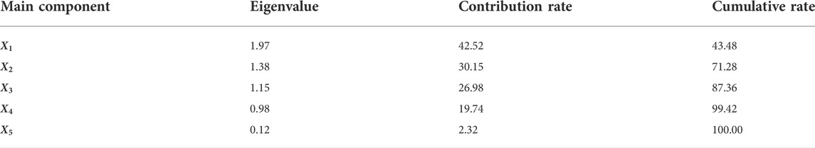
TABLE 1. Eigenvalue of covariance matrix of five variables.
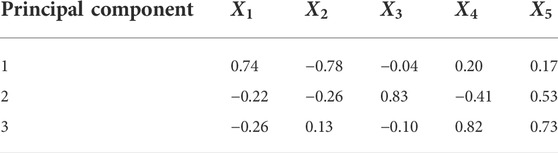
TABLE 2. Proportion coefficient of the principal component.
The sample values of the first three principal component analyses can be obtained as follows:
The weighted summation is calculated on the basic contribution rate of each attribute to produce a complete and accurate meteorological factor (A.M.F):
The comprehensive meteorological factor and solar irradiance at predicting moment, as well as 15 min during forecasting time, are the input components for the proposed system.
The accuracy and supremacy of the PCA-GWO-GRNN model are validated by forecasting the outcome of the PV plant using GWO-GRNN, PCA-LSTM, PCA-PSO-BP, and the proposed method from July 4 to 31 July 2021. Among them, the four models use the same similar day selection method as discussed in the following sections, and both input data point and output data point are nearly the same. The neural network and its proposed algorithm are developed with MATLAB 2020(b), and PCA is built with Statistical package. Figure 7 shows the solar irradiation per hour basis.
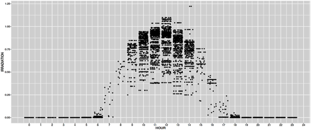
FIGURE 7. Graph between solar irradiation vs. hour.
Figure 8 depicts the forecasting and actual PV output curves on a sunny day. The projection plots of the different models are all close to the original graph, and the suggested framework produces the nearest outcome to the actual PV output.
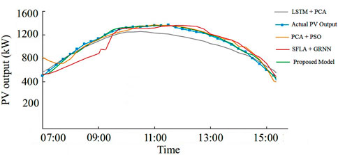
FIGURE 8. Outcome of all models of PV forecasting during sunny condition.
On a hazy day, production cloud surface area and mobility seem to be hard to predict in cloud cover in comparison to a sunny day. The PV output dramatically changes between 12:00 (afternoon) and 17:00 (evening), and the four forecasting curves and the actual curve have a huge variance. For periods with large forecasting errors, the proposed model has forecasting curves closer to the original graph, which can substantially reduce forecasting errors.
Figure 9 depicts the PV production predicting and actual curves on a wet day. During rainy days, PV production seems to be more unreliable and erratic. All four methods’ predicting findings diverge considerably from the actual curve. However, the recommended model’s slope is closer to the real curve.
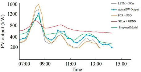
FIGURE 9. Outcome of all models of PV forecasting during rainy Conditions.
Table 3 demonstrates a comparison of precision for Figures 10, 11. According to Table 3, the recommended model’s average nMAE is 2.33%, which is 2.02%, 1.38%, and 2.30% lower than the GWO-GRNN, PCA-LSTM, and PCA-PSO-BP models, respectively. The average RMSE is 129.425 kW, considerably lower than that of the other proposed theories. The findings demonstrate that the proposed model outperforms others in day-ahead short-term photovoltaic output predicting.
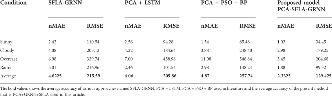
TABLE 3. Comparison of accuracy.
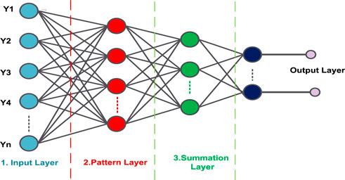
FIGURE 10. Working of GRNN.
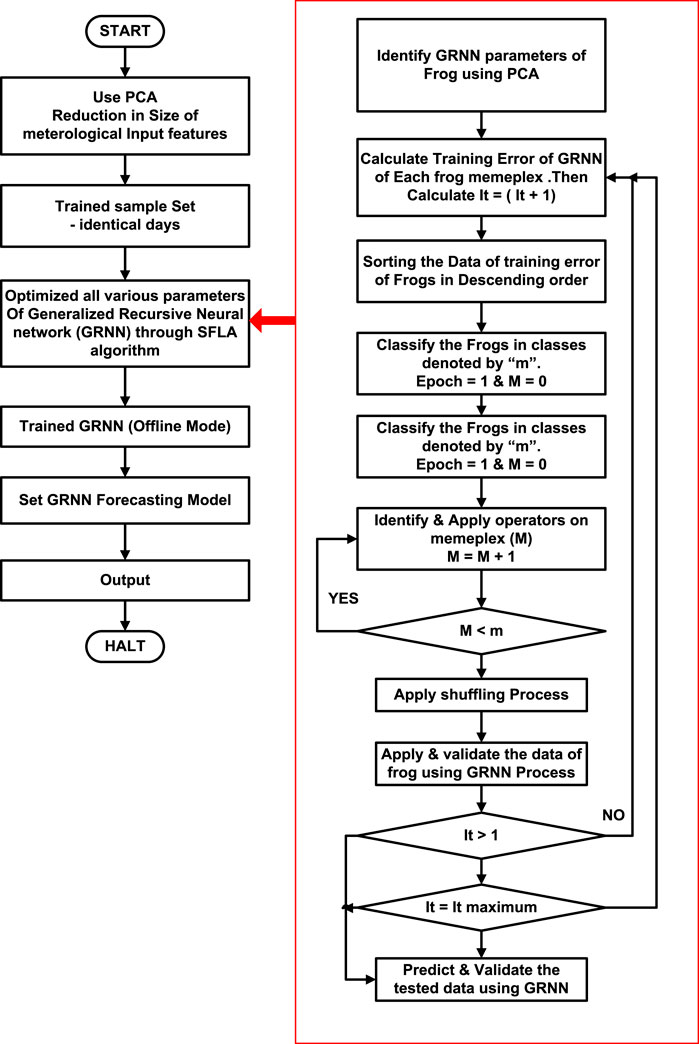
FIGURE 11. Flowchart of proposed model using PCA-SFLA-GRNN.
Because of the large dispersion of a daily error in forecasting, the error of different weather conditions for 1 month, that is, 30 days, is shown in Table 4 to further analyze the performance.
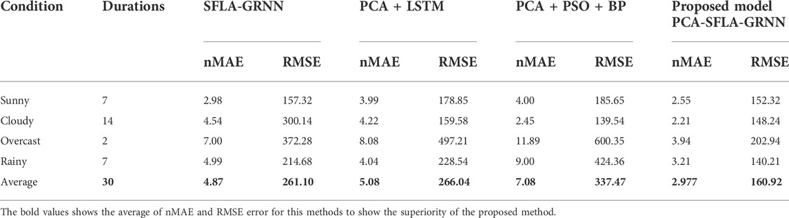
TABLE 4. Error in forecasting at different weather conditions.
According to the aforementioned analysis, the PCA-GWO-GRNN model outperforms than the other three models in terms of accuracy with respect to the different types of weather conditions. Even though the forecasting error of PV output on an overcast day is 3.94%, which is significantly worse than the forecasting accuracy of the other weather types, in general, the PCA-GWO-GRNN model has lower nMAE and RMSE than the other three models. As a result, the proposed model is more accurate.
The error obtained during PV power forecasting using different algorithms is shown in a box chart form shown in Figure 12.
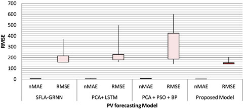
FIGURE 12. Box chart of error in forecasting using different algorithms.
The PCA-SFLA-GRNN model developed during this research tackles the issue of a high number of input variables and high variability in day-ahead short-term PV output prediction. The relevant advancements are made through this article:
i) The minimization of the size of meteorological input features is done here by PCA. It also extracted variables that comprise over 85% of the source data.
ii) It can also reduce the dimensionality of the model input data while maintaining quality and accuracy.
iii) The proposed hybrid algorithm BP-SFLA-GRNN is used to forecast PV output power in this work. The simulation outcomes show that the suggested technique outperforms the previously presented framework and the traditional way of developing GRNN.
iv) The analysis shows that the predicting model proposed in this study fully exhumes the accurate data in the input attributes with high stability and predicting precision that can provide efficient strategies to day-ahead short-term forecasting of PV output power and serve as a foundation for the optimal operation of the energy management systems.
The raw data supporting the conclusion of this article will be made available by the authors, without undue reservation.
All authors listed have made a substantial, direct, and intellectual contribution to the work and approved it for publication.
The authors declare that the research was conducted in the absence of any commercial or financial relationships that could be construed as a potential conflict of interest.
All claims expressed in this article are solely those of the authors and do not necessarily represent those of their affiliated organizations, or those of the publisher, the editors, and the reviewers. Any product that may be evaluated in this article, or claim that may be made by its manufacturer, is not guaranteed or endorsed by the publisher.
Alblawi, A., Said, T., Talaat, M., and Elkholy, M. H. (2022). “PV solar power forecasting based on hybrid MFFNN-ALO,” in 13th international conference on electrical engineering (Egypt: ICEENG), 52–56. doi:10.1109/ICEENG49683.2022.9782040
Asrari, A., Wu, T. X., and Ramos, B. (2017). A hybrid algorithm for short-term solar power prediction—sunshine state case study. IEEE Trans. Sustain. Energy 8 (2), 582–591. doi:10.1109/tste.2016.2613962
Chen, C., Duan, S., Cai, T., and Liu, B. (2011). Online 24-h solar power forecasting based on weather type classification using artificial neural network. Sol. Energy 85 (11), 2856–2870. doi:10.1016/j.solener.2011.08.027
Eseye, A. T., Zhang, J., and Zheng, D. (2018). Short-term photovoltaic solar power forecasting using a hybrid wavelet-PSO-SVM model based on SCADA and meteorological information. Renew. Energy 118, 357–367. doi:10.1016/j.renene.2017.11.011
Ge, L., Xian, Y., Yan, J., Wang, B., and Wang, Z. (2020). A hybrid model for short-term PV output forecasting based on PCA-GWO-GRNN. J. Mod. Power Syst. Clean Energy 8 (6), 1268–1275. doi:10.35833/mpce.2020.000004
Haque, A. U., Nehrir, M. H., and Mandal, P. (2013). Solar PV power generation forecast using a hybrid intelligent approach. IEEE Power & Energy Soc. General Meet., 1–5. doi:10.1109/PESMG.2013.6672634
IEA (2018). Net solar PV capacity additions 2018-2020. Paris: IEA. Available at: https://www.iea.org/data-and-statistics/charts/net-solar-pv-capacity-additions-2018-2020.
Jinpeng, W., Yang, Z., Xin, G., Jeremy, G., and Xin, Z. (2022). A hybrid predicting model for the daily photovoltaic output based on fuzzy clustering of meteorological data and joint algorithm of GAPS and RBF neural network. IEEE Access 10, 30005–30017. doi:10.1109/access.2022.3159655
Kroposki, B. (2017). Integrating high levels of variable renewable energy into electric power systems. J. Mod. Power Syst. Clean. Energy 5, 831–837. doi:10.1007/s40565-017-0339-3
Kushwaha, V., and Pindoriya, N. M. (2019). A SARIMA-RVFL hybrid model assisted by wavelet decomposition for very short-term solar PV power generation forecast. Renew. Energy 140, 124–139. doi:10.1016/j.renene.2019.03.020
Lara Fanego, V., Ruiz-Arias, J., Pozo-Vazquez, D., Santos-Alamillos, F., and Pescador, J. (2012). Evaluation of the WRF model solar irradiance forecasts in Andalusia (southern Spain). Sol. Energy 86, 2200–2217. doi:10.1016/j.solener.2011.02.014
Lin, P., Peng, Z., Lai, Y., Cheng, S., Chen, Z., and Wu, L. (2018). Short-term power prediction for photovoltaic power plants using a hybrid improved Kmeans-GRA-Elman model based on multivariate meteorological factors and historical power datasets. Energy Convers. Manag. 177, 704–717. doi:10.1016/j.enconman.2018.10.015
Mei, F., Pan, Y., Zhu, K., and Zheng, J. (2018). A hybrid online forecasting model for ultra short-term photovoltaic power generation. Sustainability 10 (3), 820. doi:10.3390/su10030820
Pan, M., Li, C., Gao, R., Huang, Y., You, H., Gu, T., et al. (2020). Photovoltaic power forecasting based on a support vector machine with improved ant colony optimization. J. Clean. Prod. 277, 123948. doi:10.1016/j.jclepro.2020.123948
Paulescu, M., Paulescu, E., Gravilla, P., and Badescu, V. (2013). “Weather modeling and forecasting of PV systems operation,” in Green energy and technology (London: Springer). doi:10.1007/978-1-4471-4649-0
Pretto, S., Ogliari, E., Niccolai, A., and Nespoli, A. (2022). A new probabilistic ensemble method for an enhanced day-ahead PV power forecast. IEEE J. Photovolt. 12 (2), 581–588. doi:10.1109/jphotov.2021.3138223
Ramakrishna, R., Scaglione, A., Vittal, V., Dall’Anese, E., and Bernstein, A. (2019). A model for joint probabilistic forecast of solar photovoltaic power and outdoor temperature. IEEE Trans. Signal Process. 67 (24), 6368–6383. doi:10.1109/tsp.2019.2954973
Raza, M. Q., Mithulananthan, N., Li, J., Lee, K. Y., and Gooi, H. B. (2019). An ensemble framework for day-ahead forecast of PV output power in smart grids. IEEE Trans. Ind. Inf. 15 (8), 4624–4634. doi:10.1109/tii.2018.2882598
Raza, M. Q., Nadarajah, M., and Ekanayake, C. (2016). On recent advances in PV output power forecast. Sol. Energy 136, 125–144. doi:10.1016/j.solener.2016.06.073
Rosato, A., Panella, M., and Araneo, R. A. (2019). A distributed algorithm for the cooperative prediction of power production in PV plants. IEEE Trans. Energy Convers. 34 (1), 497–508. doi:10.1109/tec.2018.2873009
Theocharides, S., Makrides, G., Livera, A., Theristis, M., Kaimakis, P., and Georghiou, G. E. (2020). Day-ahead photovoltaic power production forecasting methodology based on machine learning and statistical post-processing. Appl. Energy 268, 115023. doi:10.1016/j.apenergy.2020.115023
Yang, H. T., Huang, C. M., Huang, Y. C., and Pai, Y. S. (2014). A weather based hybrid method for 1-day ahead hourly forecasting of PV power output. IEEE Trans. Sustain. Energy 5 (3), 917–926. doi:10.1109/TSTE.2014.2313600
Zhang, T., Lv, C., Ma, F., Zhao, K., Wang, H., and O'Hare, G. M. P. (2020). A photovoltaic power forecasting model based on dendritic neuron networks with the aid of wavelet transform. Neurocomputing 397, 438–446. doi:10.1016/j.neucom.2019.08.105
Zhou, Y., Zhou, N., Gong, L., and Jiang, M. (2020). Prediction of photovoltaic power output based on similar day analysis, genetic algorithm and extreme learning machine. Energy 204, 117894. Art. no. doi:10.1016/j.energy.2020.117894
Keywords: photovoltaic output forecasting, solar power prediction, generalized regression neural network (GRNN), shuffled frog leaping algorithm (SFLA), performance indexes
Citation: Gupta AK and Singh RK (2022) Short-term day-ahead photovoltaic output forecasting using PCA-SFLA-GRNN algorithm. Front. Energy Res. 10:1029449. doi: 10.3389/fenrg.2022.1029449
Received: 27 August 2022; Accepted: 26 September 2022;
Published: 21 October 2022.
Edited by:
Mawloud Guermoui, Applied Research Unit for Renewable Energies, AlgeriaReviewed by:
Abdelaziz Rabehi, Ziane Achour University of Djelfa, AlgeriaCopyright © 2022 Gupta and Singh. This is an open-access article distributed under the terms of the Creative Commons Attribution License (CC BY). The use, distribution or reproduction in other forums is permitted, provided the original author(s) and the copyright owner(s) are credited and that the original publication in this journal is cited, in accordance with accepted academic practice. No use, distribution or reproduction is permitted which does not comply with these terms.
*Correspondence: Ankur Kumar Gupta, YW5rdXJrb3J3YTFAZ21haWwuY29t
Disclaimer: All claims expressed in this article are solely those of the authors and do not necessarily represent those of their affiliated organizations, or those of the publisher, the editors and the reviewers. Any product that may be evaluated in this article or claim that may be made by its manufacturer is not guaranteed or endorsed by the publisher.
Research integrity at Frontiers
Learn more about the work of our research integrity team to safeguard the quality of each article we publish.