 Matthieu Dubarry
 David Anseán
- 1Hawai’i Natural Energy Institute, University of Hawai’i at Mānoa, Honolulu, HI, United States
- 2Department of Electrical Engineering, Polytechnic School of Engineering, University of Oviedo, Gijon, Spain
This publication will present best practices for incremental capacity analysis, a technique whose popularity is growing year by year because of its ability to identify battery degradation modes for diagnosis and prognosis. While not complicated in principles, the analysis can often feel overwhelming for newcomers because of contradictory information introduced by ill-analyzed datasets. This work aims to summarize and centralize good practices to provide a strong baseline to start a proper analysis. We will provide general comments on the technique and how to avoid the main pitfalls. We will also discuss the best starting points for the most common battery chemistries such as layered oxides, iron phosphate, spinel or blends for positive electrodes and graphite, silicon oxide, or lithium titanate for negative electrodes. Finally, a set of complete synthetic degradation maps for the most common commercially available chemistries will be provided and discussed to serve as guide for future studies.
1 Introduction
Efficient non-invasive techniques to establish Li-ion battery diagnosis, prognosis, and state of safety are keys to accelerate the deployment of large battery systems. Among the available techniques, the electrochemical voltage spectroscopies that are derivatives of the voltage response of a battery are especially relevant because they solely rely on sensors commonly available in commercial battery systems (i.e., current and voltage sensing). Moreover, because of the derivation, the resulting curves display large variations that can be easily measured and compared. These variations are related to material chemistry and, thus, provide thermodynamic information on the internal state of the battery. Among those techniques, the popularity of incremental capacity (IC) analysis (A) (dQ/dV = f(V)) is growing steadily year by year. This is accompanied by an ever-increasing number of publications, and similar to what was reported by Xu (2022) for electrolytes, the IC-related literature is now a minefield with frequent inaccuracies and fundamental errors. This is mostly induced by the fact that the analysis is chemistry dependent and that a tool used on one chemistry might not be applicable to others. This work aims to establish a set of best practices for accurate IC analysis, while providing a strong theoretical background and addressing the most common issues found when applying this technique. In addition, a set of synthetic degradation maps for the most common commercially available chemistries, as well as exemplary degradation examples, will be provided to illustrate the discussion and provide a training set for newcomers. This work will focus on experimental data analysis rather than modeling. For modeling, interested readers can refer to Dubarry et al. (2012); Dubarry and Beck (2022); and an article by Weng et al. (2022) in this issue for applications.
The IC and its inverse technique, differential voltage (DV) analysis (dV/dQ = f(Q)) introduced by Bloom et al. (2005), are both non-invasive techniques well suited to establish battery diagnosis from laboratory testing or field data. They enable quantification of the degradation modes (Birkl et al., 2017), an intermediate between the simple capacity/resistance monitoring and the full post-mortem investigation (Waldmann et al., 2016) of degradation mechanisms, providing a good balance between accuracy and required resources (Dubarry et al., 2020). Both techniques yield the highest accuracy results when used on low-rate constant current data. The accuracy of the analysis will be reduced by higher current, low resolution, and noisiness. Application outside of constant current is more complicated without a strong model (Dubarry and Beck, 2022). Compared to DVA, the main benefit of ICA is that IC is sensitive to resistance changes so that they could be quantified without any additional experiments such as electrochemical impedance spectroscopy. Other significant benefits are that blends contribution are additive (Smith et al., 2012; Schmidt et al., 2013) and that the x-axis is constant throughout the life of the cells. This prevents the need for rescaling and it allows working on partial charges or discharges. The main drawback of IC compared to DV is that the contribution of the positive (PE) and negative (NE) electrodes is convoluted (vs. additive for DV), which can make their individual impact difficult to assess at first glance. This can be overcome by careful peak indexation (Dubarry et al., 2011a; Barai et al., 2019; Dubarry and Baure, 2020). More comparisons between the two techniques can be found in Barai et al. (2019).
Another important aspect to highlight is that there are two levels for ICA or DVA analysis, namely, high and low (Barai et al., 2019). These derivative techniques enhance the changes in the voltage response through usage and, as such, at a high level, they give a much better picture of the state of the cell than the traditional voltage vs. capacity curves without any need for analysis. This is extremely useful to validate accelerated aging protocols—must have the same voltage response after same capacity loss to equal same degradation—or validate models claiming to replicate the electrochemical response of the cells—must have the same peaks at the same potentials to equal replication of all reactions. This publication will address the lower level by providing a guide on how to make sense of the voltage changes. ICA could not only be used to analyze aging (cycle or calendar) but also electrochemical milling (Dubarry et al., 2014), decomposition of additives (Khodr et al., 2020), lithium plating (Anseán et al., 2017; Chen et al., 2022), the impact of temperature (Dubarry et al., 2013; Fly et al., 2022; Gauthier et al., 2022), inhomogeneities (Fath et al., 2019), fast charge (Tanim et al., 2018), hysteresis (Dubarry et al., 2008), overdischarge (Zhang et al., 2022), and many other aspects.
2 General comments
All the data presented in this work are stock data from the ‘alawa toolbox, which is available for free for academic users (https://www.soest.hawaii.edu/HNEI/alawa/). No experiments were specifically performed for this publication. The use of synthetic data enables to focus only on the core aspects and simplifies the discussion by limiting data description. When available, the reference publication where the data were first used will be added. Most of the data used in this work were made publicly available (Dubarry and Anseán González, 2022). Because normalized synthetic data are used, the unit of the IC curves will be %Q/V instead of the usual Ah/V, and resistance values will be in Ω.Ah instead of Ω. For obvious reasons, and to the best of our knowledge, no publications with erroneous ICA analysis will be cited in this work, but given the extent of the literature on the subject, we would like to emphasize that they only account for a fraction of the non-cited articles.
2.1 IC curve derivation
This section will address 1) the impact of sampling frequency and 2) the impact of smoothing the voltage curve vs. smoothing the IC curve. The accuracy of the diagnosis will be significantly impacted by the quality of the data. It is best to gather data with well-calibrated equipment, with as good resolution as possible, 1 mV or below is preferred. Moreover, to reduce environmental and procedural errors further, it is important to ensure environmental consistency throughout the testing (temperatures and contacts). The sampling rate should also be limited to avoid large data files. Recording 2000 points per regime is sufficient to carry an ICA. IC curves are generally plotted at low rates (C/10 or below with C/25 preferred) to investigate the thermodynamical aspects. At higher rates, the IC signature will be influenced by both thermodynamic and kinetic aspects and might be harder to decipher. Best practices for testing are out of the scope of this work and are available in Dubarry and Baure (2020).
To calculate the IC curves, our preferred solution is to apply a filter that considers one data point every set number of mV, typically 2 mV. As a rule of thumb, similar to that of X-ray diffraction, the aim is to maintain at least five points above each peak half-width to trust their position and intensity. If necessary, a smoothing function could be applied on the voltage data before derivation to reduce the noise further. In both cases, it is essential to verify that the shape and position of the peaks were not affected by filtering and/or smoothing. Figure 1 presents an illustration of the impact of filtering and smoothing on the IC response of a graphite intercalation compound (GIC)/lithium iron phosphate (LFP) cell during discharge. Figure 1A presents the impact of the filtering, from no filtering to 8 mV steps. The data with the 1 mV step are still noisy, while some peaks were starting to be displaced for the 4 mV step data (circle on Figure 1A). The data after the 8 mV filtering significantly deformed the peaks. The 1 mV step data could still be used with further smoothing, (Figure 1B). For this example, the smoothing was performed using the MATLAB© smooth function at different levels, using 1%–10% of the data. In this example, the 5% smoothing starts to move the peaks, and this is even more evident on the 10% data (circle on Figure 1A). Figure 1B also showcases the difference between smoothing before (full lines) or after (dashed lines) the derivation. Smoothing after derivation is inducing much more distortion of the data and should be avoided. This is explained by the fact that the voltage curve is monotonically decreasing during discharge whereas the IC curve is not. Referring to the literature, Li et al. (2018) and Liu et al. (2022) also looked at the impact of filtering. Last, it is worth mentioning that some authors also managed to extract high resolution curves using probability functions (Feng et al., 2013) and a level evaluation analysis (Feng et al., 2020). Both these methods could prove useful to reduce noise further if necessary.
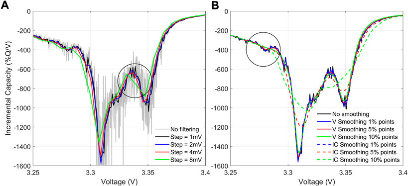
FIGURE 1. (A) Impact of filtering and (B) smoothing on a C/25 GIC/LFP discharge cycle.
2.2 Making sense of IC curves: Theoretical aspects
Understanding IC curves requires some knowledge of 1) the electrochemical behavior of the electrodes, 2) the clepsydra analogy, and 3) the concept of degradation modes.
Because of the structural changes induced by lithiation/delithiation, the voltage of electrode materials will change alongside lithium concentration. Reactions can mainly occur as phase transformations or solid solutions (Huggins, 2016). Both have compositionally the same starting and ending point, but the path differs. Using an analogy and imagining a bag of marbles starting with white and progressively becoming black, a solid solution corresponds to all the marbles getting grayer and grayer together until black. The phase transformation corresponds to marbles going one-by-one from white to black instantly. During solid solution, the structure changes with composition, and this results in a varying voltage and broadening of the IC peak. During the phase transformation, the structure and composition of the new and old phases are constant and only their ratio is changing. This results in a voltage plateau and a sharp IC peak. Readers interested by the thermodynamic explanation can refer to Huggins (2016).
Each electro-active material will go through its own unique set of structural changes through intercalation/deintercalation and therefore has a unique voltage signature. Figure 2 presents exemplary incremental capacity curves, showcasing the unique electrochemical behavior of all the electrodes used in this work. The main reactions will be numbered in white from high to low voltage for the PE and in black from low to high voltage for NE. Numbering is reversed for the NE because it is going through the opposite regime to that of the PE. By convention, the IC peaks in discharge should be negative and the one in charge should be positive. Starting with the top row, LiCoO2 (LCO), LiNixMnyCozO2 (NMCxyz) with x,y,z = [1,1,1] and [5,3,2] (NMC111 and NMC532) share a lot of similarities in their electrochemical behavior. The response is mainly made of a broad shoulder at high voltage (➀) and a well-defined peak at low voltage (➁). For LCO, it has to be noted that, depending on the synthesis method and coatings, two small peaks could be present in the middle of shoulder ➀ (Reimers and Dahn, 1992). For the NMCs, peak ➁ is broad in discharge and could have two components in charge. For higher Ni concentration in NMC, NMC811, the electrochemical response is more complex with five clearly identifiable peaks (➀–➄), including a very sharp peak at high voltage (➀). The intensity of this peak is composition-dependent and might vary between samples from different manufacturers. For more details on the effect of chemical composition on the response of NMC, interested readers are referred to MacNeil et al. (2002); Noh et al. (2013). Continuing with the second row, nickel cobalt aluminum oxide (NCA) shares some similarities with the low Ni-layered oxides, but four peaks are observed (➀ to ➃). Lithium manganese oxide (LMO) presents an interesting electrochemical response with some capacity at high voltage with two peaks (➀ and ➁) and some capacity at low voltage (➂) with no electrochemical activity in-between. The low voltage capacity (peak ➂) is not accessible in GIC/LMO cells because there is not enough lithium to start with but it could be accessible in the case of blends (Dubarry et al., 2015). LFP presents a single peak in charge and discharge (➀) around 3.43 V. The third row showcases the NEs, first GIC presents three well-marked peaks (➊,➋, and ➎) and two small peaks that might be hard to see for some graphites (➌ and ➍). Lithium titanium oxide (LTO) presents a signature similar to LFP but at a voltage around 1.55 V. Finally, silicon (Si) showcases two broad peaks (➊ and ➋). It has to be noted that materials from different manufacturers, batches, or synthetized differently might not have exactly the same response as the materials showcased in Figure 2 but the described trends should be similar.
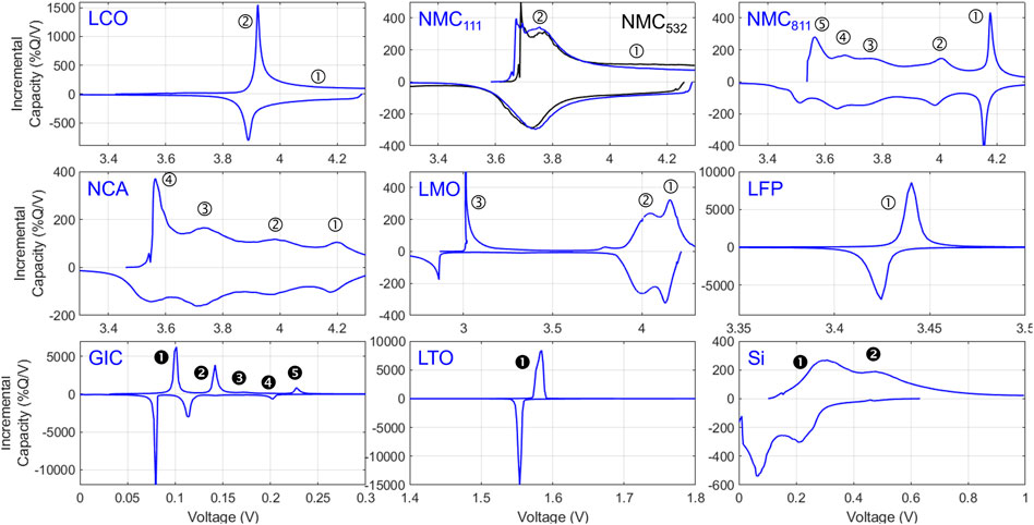
FIGURE 2. Exemplary C/25 electrochemical behavior for all the material used in this work.
The next stage is to understand how the PE and NE interact with each other at the full cell level. As explained in Dubarry et al. (2011a); Barai et al. (2019); Dubarry and Baure (2020), this can be seen as a communicating vessel problem. To ease the discussion, and to kill two birds with one stone, Figure 3 presents an example of the process for a blended (NMC0.75, LMO0.25) PE vs. graphite. Figure 3A showcases the response of the blend vs. metallic Li to exemplify that the response of the blends is the sum of the pondered response of the individual components. This is because the potential of an electrode will only change when all the lithium available at the current voltage are exchanged, independently of where they are coming from. Figure 3B presents the complex response of the full cell when the blend is associated with graphite at the NE. Comparing the peaks from Figure 3B to the ones of the PE (Figure 3A) and the NE (GIC on Figure 2), the correspondence is not evident because each peak on the IC curve corresponds to the convolution of each electrode response. The key is to realize that the lithium going back and forth between the electrodes could be seen as a liquid going back and forth between two bulbs in a clepsydra, or water clock. The shape of the bulb is going to define how the height of the liquid in each bulb will be changing when liquid is transferred. In this analogy, the height of the liquid represents potential energy, which is analogous to voltage. For the voltage of a bulb to match the half-cell response of the electrode when it is emptied, it has to be shaped as the IC curve (Dubarry and Baure, 2020) as, assuming a constant flow, for each voltage V, the corresponding volume of liquid to remove to change the voltage by dV is dQ/dV. The clepsydra is represented schematically in Figure 3C. At the beginning of the discharge, nearly all the lithium is in the NE. The corresponding bulb is nearly full and there is liquid up to the lowest voltage peak ➊. The PE is almost empty and this corresponds to only a little liquid in the bottom area, ➀NMC. The corresponding feature on the IC curve can thus be labeled ➊★➀NMC as it corresponds to the voltage difference between these reactions in each electrode. If some capacity is passed, the liquid height in the NE will go down, whereas it will go up in the PE. Therefore, the difference between the heights in the two bulbs, that is, the voltage of the cell, will go down. Taking an example toward mid-discharge, the NE could be filled up to peak ➋ and the PE to peak ➁NMC. The corresponding peak will thus be ➋★➁NMC on the full cell IC curve. At the end of the discharge, the NE is nearly empty on peak ➎, whereas the PE is finishing peak ➁NMC. A different way of visualizing the same concept with more emphasis on capacity for each electrode, or component of, is presented in Figure 3D (Dubarry et al., 2011a). A new feature will be visible on the IC curve every time there is a reaction change in any of the electrodes.
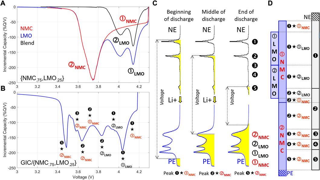
FIGURE 3. (A) IC signature of a (NMC.75, LMO.25) blend with a 3/1 ratio vs. metallic Li, (B) signature vs. graphite. (C) Clepsydra analogy, and (D) capacity equivalence for easier full indexing.
It can be noticed on Figure 3D that some of the PE capacity is not used at low voltage (dashed area on bottom), and reciprocally some capacity of the NE is not used at high voltage (dashed area on top). This is because typical GIC-based cells are oversized, carrying an excess of NE to prevent lithium plating at the edges of the graphite anode. For the PE, some capacity is not used because the solid electrolyte interphase (SEI) formation and growth during formation consumes Li-ion, which prevent the PE to be fully lithiated back. Therefore, to properly describe the matching of the electrodes, it is necessary to estimate the excess on both sides. This could be performed by quantifying the ratio of capacity between the NE and the PE, the loading ratio (LR), and their offset (OFS), Figure 4A (Dubarry et al., 2012). The initial LR and OFS are usually varying from manufacturer-to-manufacturer, from cell to cell because of manufacturing variability (Devie and Dubarry, 2016), and from differences in architecture (e.g., high power vs. high energy (Dubarry et al., 2014)). From experience, the offset is generally small for GIC/layered oxide-based cells (2–5%) because some PE is lost alongside the SEI layer formation in the first cycles (Devie and Dubarry, 2016). This is also true for LTO-based cells because there is little to no SEI formation (Baure et al., 2019). This however is not the case for GIC/LFP-based cells where the offset could be larger (7–12%) (Anseán et al., 2016) because the PE is stable through initial intercalation/deintercalation.
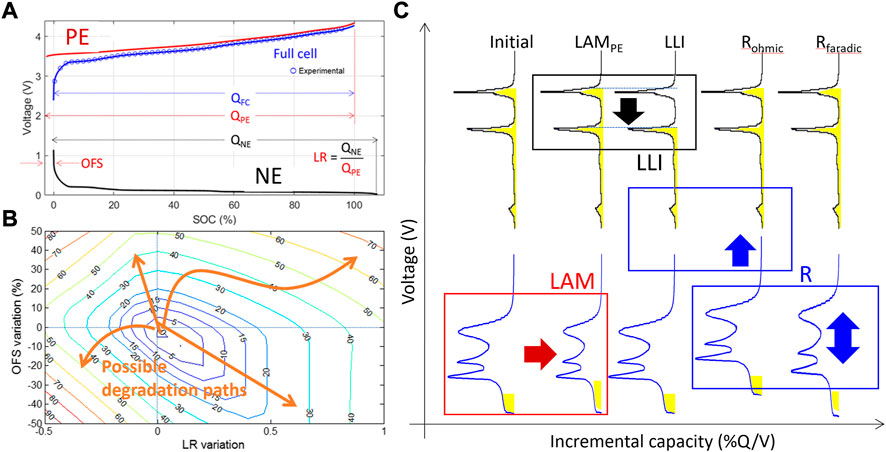
FIGURE 4. (A) Representation of the relationship between the PE, NE, and full cell. (B) Exemplary contour plot showcasing evolution of capacity loss as a function of the variations of LR and OFS. (C) Clepsydra analogy for the impact of LAM, LLI, and R changes, both ohmic and faradic. Adapted from Barai et al. (2019); Dubarry and Baure (2020).
Assuming that the electrochemical behavior of the electrodes does not change with time, which is true for most commercial electrodes at the moment, battery degradation only affects their matching. Figure 4B presents the impact of varying LR and OFS on capacity loss. This highlights how an infinite amount of degradation paths can lead to the same capacity loss. When only looking at thermodynamics, diagnosing cell degradation equates to finding the new LR and OFS after aging. Kinetics will induce further changes such as variations in ohmic and faradic resistances. While describing changes of parameters is enough to provide a diagnosis, it lacks physical meaning. Fortunately, their variations can be linked to the degradation modes, a set of metrics representative of the changes within a cell (Birkl et al., 2017; Dubarry et al., 2020; Dubarry and Beck, 2022). Degradation modes refer to the impact of degradation mechanisms on the electrode voltage response rather than their root cause. They comprise the loss of lithium inventory (LLI), the loss of active material (LAM), and kinetic limitations (KL) because every degradation process can always be decomposed to its impact on the amount of material able to react, on the amount of lithium able to go back and forth, and on the overall electrode kinetics (Dubarry and Beck, 2022). KL should be decomposed further into ohmic and faradic contributions. LAM and KL are electrode-specific and even material-specific for blends (Baure et al., 2019). More details on the concept of degradation modes can be found in Dubarry et al. (2012); Birkl et al. (2017). In addition, readers interested in IC when the electrochemical behavior of the electrodes changes with time can refer to Rodrigues et al. (2022) and Dubarry and Beck (2022).
Going back to the clepsydra analogy, it also allows illustrating the impact of the degradation modes on the electrode matching, (Figure 4C) (Barai et al., 2019). In case of LAM, one bulb becomes smaller compared to the other but the volume of lithium remains the same. This will change the filling of the affected electrode and thus the voltage response of the cells. This will also predominantly affect the LR. LR will increase in case of LAMPE and decrease in case of LAMNE. In case of LLI, the electrodes are untouched but some lithium is missing, therefore the NE cannot be filled to the same level at the end of charge. In other words, there is a leak in the clepsydra. LLI is the main contributor to the increase of the offset. In case of increase of ohmic resistance, the two bulbs are getting closer together in discharge (average voltage decreases) and farther away in charge (average voltage increase). This might not be associated with any capacity loss initially (Attia et al., 2022). In case of change of faradic resistance, the shape of the peaks is altered with the peaks getting broader with worsening kinetics, for example, increasing rate (Schindler et al., 2019) or decreasing temperature (Dubarry et al., 2013; Fly et al., 2022). An example is presented in Figure 5A. Interested readers can find a full set of equations in (Dubarry et al., 2012).
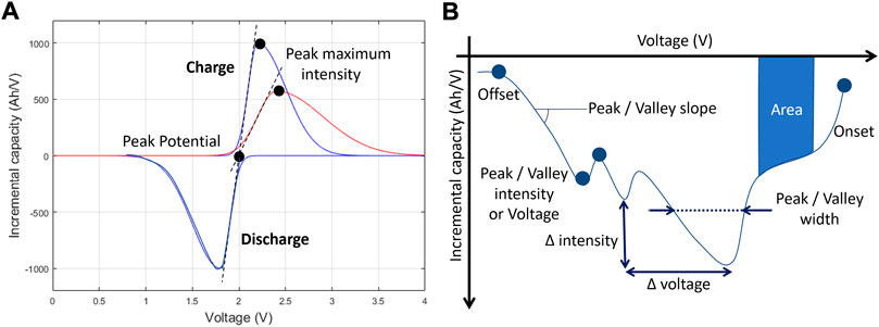
FIGURE 5. (A) Ideal IC peak for two different kinetic values and (B) other possible FOIs. Adapted from Dubarry and Baure (2020).
2.3 Initial steps for analysis
Because every chemistry presents a different electrochemical behavior, Figure 2, and because every battery will have its own set of LR and OFS, it is recommended to always start from a degradation map. A degradation map is a compilation of synthetically generated curves (Dubarry et al., 2012), representing the voltage variations associated with single degradation modes (e.g., only LLI, only LAMPE). These synthetic curves help decipher which part of the curve is most sensitive to a specific degradation mode. Degradation maps usually consist of several panels showcasing the impact of a specific degradation mode individually on the voltage response of the cell. The last panel often showcases the evolution of the capacity loss along the degradation modes. Degradation maps are available in the literature for most chemistries and are collected here for convenience with the associated publication if available. Corresponding data can be found in Dubarry and Anseán González (2022).
Before looking at the degradation map, it is important to discuss how to describe IC curves. First and foremost, the voltage of the peak maximum intensity is not its position as the peak position is the front of the peak. This is because the reaction is starting at a given potential (the redox potential), which is the same in charge and discharge. In discharge, the reaction will only occur below this potential. In charge, the reaction will only occur above this potential. This is exemplified in Figure 5A with the IC curves for an ideal phase transformation with two different kinetics in charge (blue: fast and red: slow). In this example, the position of the peak did not change with kinetics, it only broadened. With the decrease of the front slope of the peak, the position of the maximum intensity will move but the reaction remained the same. For perfect phase transformations, and at low rate, the peaks in charge and discharge should be perfectly aligned like in Figure 5A. If not, a potential hysteresis can be discussed.
It is also important to realize that features other than peaks can be used for efficient ICA, Figure 5B. Depending on the case figure, features of interest (FOI) can be defined from the onset, position, intensity, width, front slope, back slope, area, or offset. The choice of FOI will depend on the chemistry, voltage window, and regime (Dubarry et al., 2017; Dubarry and Beck, 2021). FOIs description for the main commercially available chemistries will be provided in Section 3 of this work.
The goal of an ICA analysis is to quantify the degradation modes. For a non-blended system, there are six unknowns: the three thermodynamic modes LLI, LAMPE, and LAMNE, and three kinetic ones, the ohmic resistance increase (ORI), and the faradic rate degradation (FRD) on the PE and NE (Dubarry et al., 2012). This is a logical but qualitative process of elimination approach starting from the experimental data and the associated degradation map.
ORI is the easiest to assess as, if the charge or discharge always starts from the same state of charge, it can be easily quantified from the evolution of the initial voltage drop (Dubarry and Baure, 2020). If the IC intensity comes back to zero at the end of discharge upon aging, it can also be determined that the resistance increase does not induce any capacity loss (Attia et al., 2022).
The second mode that is easily quantifiable is the one responsible for the capacity loss. This corresponds to identifying which electrodes are limiting at end of charge (EOC) and end of discharge (EOD) and this is chemistry and parameter dependent. Figure 6 presents a schematic representation of the four possible cases figures for the limiting electrodes with the associated equations linking capacity loss and degradation modes. If the PE is limiting at EOC and the NE at EOD, as in a traditional graphite-based battery at beginning of life (BOL), the capacity loss is driven by LLI because there is a “reservoir” of PE and NE on each side as discussed earlier. Therefore, before the LAMs are high enough to change the limiting electrodes, they are hidden degradation modes and are associated with little to no capacity loss. This exemplifies why degradation and capacity loss must be decorrelated. For quantification, it is important to realize that, for Li-ion systems, the entirety of the lithium is provided by the PE, therefore the relationship between LLI and capacity loss needs to be pondered by the capacity ratio between the PE and the full cell. If the NE is limiting on both ends, as in a typical LTO-based cell at BOL (Baure et al., 2019; Baure and Dubarry, 2020), the capacity loss is driven by LAMNE. If the full cell capacity is smaller than the one of the NE, the ratio of LAM/capacity loss will not be 1:1. In addition, in this case figure, LLI and LAMPE are hidden modes because they have a “reservoir.” If the PE is limiting on both ends, the capacity loss is unsurprisingly driven by LAMPE while LLI and LAMNE are hidden. The fourth configuration (NE limiting at EOC and PE at EOD) is more complex with a capacity loss induced by both LAMs with LLI only as a hidden mode. It has to be noted that the provided equations are true for electrodes with a perfect plateau and at low rate. More complex voltage responses might influence the values slightly. This is what typically explains some counter intuitive effects such as increases of capacity at beginning of cycling, the fact that capacity could be lost at low rate but not at high rates (Dubarry and Liaw, 2009; Dubarry et al., 2014), or the fact that LLI could in some cases not be fully correlated with capacity loss (Weng et al., 2021).
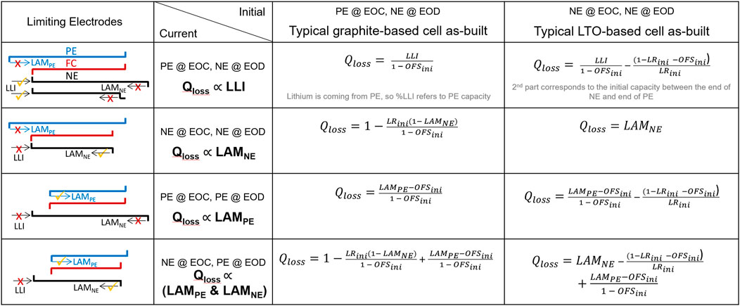
FIGURE 6. Impact of limiting electrodes on the main contributor to capacity loss with associated equations for typical graphite and LTO-based cells.
In summary, LLI is usually responsible for the initial capacity loss for graphite-based cells except for smaller voltage windows where LAMPE could not have time to be compensated. In cells for which plating could occur in the potential window, LAMNE will never be responsible for any significant capacity loss because it will be supplemented by plating. Plating can be identified in the LAMdeGIC panel with a drop in potential before coming up again in charge (* in Figure 7). Plating by itself does not induce capacity loss, only irreversible plating does by adding LLI (Attia et al., 2022). For LTO-based cells, however, capacity loss is often associated to LAMNE initially because plating is well outside the potential window. The other cases of limiting electrodes could occur upon aging.
FIGURE 7. Degradation map for a GIC/NMC cell for up to 30% of LLI and LAMs and up to 5x kinetic and resistance increases with 2% interval (thick full line: initial cycle, dotted lines: intermediate cycles, and thin full line: final cycle).
The origin of capacity loss can be deciphered following logical deductions by comparing the degradation map to the experimental data. Figure 7 presents the degradation map for a GIC/NMC to exemplify the process. Looking at capacity loss panel in the bottom right panel, it is observed that LAMPE without lithium (i.e., LAMdeNMC) is not initially associated with any capacity loss. This is because the PE is not limiting at EOD and therefore has a “reservoir” as exemplified in Figure 3D. Looking at the associated voltage response in the corresponding LAMdeNMC panel, the consumption of the reservoir is associated with a move of the lowest voltage peak ➎★➁ toward lower voltages before a gradual disappearance when the PE becomes limiting. Therefore, if this peak on the experimental data did not move, or moved toward higher voltages, the PE cannot be limiting at end of discharge and no capacity could have been lost because of LAMPE. Therefore, for low ORI changes, the capacity has to be attributed, and be directly proportional, to LLI. If the peak started to disappear, then the PE became limiting and LAMPE is responsible for the capacity loss.
Depending on the limiting electrode, the remaining two thermodynamic degradation modes within LLI, LAMPE, and LAMNE might be more complicated to decipher. The key to addressing this occurrence is to find sensitive FOIs. This is where the degradation maps provide valuable information as they provide a broad view of the possible spectrum of degradation. To help even further, the lithiated LAMs are sometimes plotted (LAMliPE and LAMliNE, as opposed to the delithiated ones de-). LAMliX is equivalent to LAMdex + LLI while LAMX and LAMdeX are the same. LAMliX are here for illustration only as it is almost impossible to determine where the lithium was lost using IC alone. To the best of our knowledge, it was performed convincingly once in a very specific case figure (Devie et al., 2016). However, plotting them allows to visualize how the FOI moves with LAMs and LLI occurring concomitantly. This is essential to monitor potential combined effects. For example, looking at the low voltage peak ➎★➁ at 3.45 V in charge, LLI is pushing the peak toward higher voltages, LAMPE toward lower potentials, and LAMNE does not move it at all (arrows and equal symbol on Figure 7). Therefore, by identifying that in case of LAMPE + LLI in a 1:1 ratio the ➎★➁ peak is not moving as much because the LLI and LAMPE impact are canceling each other, and that in case of LAMNE + LLI the ➎★➁ peak is moving at the same pace than of under LLI alone, it can be determined that ➎★➁ might be a good indicator of the LAMPE/LLI ratio. The maps are here to help define chemistry-specific logical relationships between degradation mode and voltage variations in order to eliminate any guess work. A more chemistry-specific discussion will be provided in Section 3, with associated look-up tables and degradation maps is SI (Figures S1 to S10).
Differences in peak shapes and position that still cannot be explained after ORI, LLI, and LAMs quantification might indicate some additional kinetic limitations on either electrode needs to be considered. This includes changes in rate capability or inhomogeneities. The degradation map can help showcasing how, and how much, the peaks could be moving if kinetics degraded or improved with the rate degradation factor (RDF) for kinetics and the ohmic resistance increase (ORI) for polarization.
The overall process is summarized as a flow chart in Figure 8, starting from the experimental data to first quantify eventual resistance changes, then the determination of the limiting electrodes to decipher which thermodynamic mode is responsible for capacity loss using a degradation map. The degradation map is also needed for the next two steps corresponding to the quantification of the remaining thermodynamic modes and of the kinetics using different FOIs.

FIGURE 8. Proposed flowchart for successful ICA.
2.4 Other considerations
One common question about ICA is whether to use the charge or discharge curves. Both are valid and should lead to the same results. The decision should first be based on the application. If the deployed data are more likely to be analyzed in charge (e.g., electric vehicles) then charge should be used. Inversely, if the most likely regime for analysis is the discharge, discharge should be used. The main difference between the charge and discharge curves is usually introduced by the kinetics of the PE for graphite-based cells (Dubarry and Liaw, 2009). Indeed, Figure 2 shows that graphite showcases thin peaks for graphite, whereas the peaks of the PE are usually broader. Depending on the regime, graphite peak ➎ will either be the last (discharge) or the first (in charge) to happen and, as Figure 5A displays, with asymmetric peaks, the same capacity at the end of the reaction will correspond to a bigger ΔV than that at the beginning. This is why the low voltage graphite peaks are usually much more visible in charge. Inversely, high voltage features are usually more resolved in discharge.
The “peak area analysis” is often used to analyze batteries using lithium iron phosphate (LFP) as the positive electrode (Dubarry et al., 2014; Anseán et al., 2016, Anseán et al., 2017) but is not recommended for other chemistries. This analysis is working for LFP, while the NE is limiting at EOD, because the intensity of the IC peaks goes back close to zero before the next peak start, Figure 2, therefore the capacity under the peaks is well separated. This is not the case for other chemistries, and such analysis should thus be subjected to caution. For chemistries with a well-marked transition between graphite ➊ and ➋ for both the pristine and aged cell, and while the NE is limiting at EOD, the technique could still be used to get an approximate value of LAMNE (see example in Section 4 for NMC111).
Lithium plating is usually much more visible in charge because its reversibility is usually pretty low. Before the discharge, the lithium could mostly have been intercalated back in graphite during a rest or became passivated by the electrolyte (Attia et al., 2022). Plating will usually appear as an additional peak at high voltage about 80 mV above the last graphitic peak (depending on rate and PE) (Ratnakumar and Smart, 2010; Anseán et al., 2017; Chen et al., 2022). The acceleration of the rate of LLI can be linked to the amount of irreversible lithium plating (Anseán et al., 2017) and the ratio of LAMNE/LLI can be used to predict the onset of lithium plating (Anseán et al., 2017; Baure and Dubarry, 2019), which can enable forecast of the knee in the capacity loss or resistance increase (Anseán et al., 2017; Attia et al., 2022).
One aspect that is often neglected for blended electrodes is to separate both components for LAM calculations. It is highly likely that both components of the blends are degrading at a different pace, or are affected differently by the conditions (temperature, depth of discharge, SOC...). An example of that is presented in Baure et al. (2019), with different impacts of state of charge and temperature on NCA and LCO, which was not surprising as they are not affected by the same calendar aging (Dubarry et al., 2018b). In addition, as the materials are sharing Li-ions when blended, kinetics differences can lead to overdischarge issues on some components of the blend (Dubarry et al., 2015).
As showcased recently from the analysis of packs (Dubarry et al., 2009; Tanim et al., 2021) or single cells (Lewerenz and Sauer, 2018; Sieg et al., 2020) inhomogeneities (whether in the pack as imbalance or in the single cells as local gradients) could have a significant impact on the voltage response. This will be an essential aspect to consider, and quantify, for future studies on packs or single cells. Recent models (Dubarry et al., 2019; Dubarry and Beck, 2022; von Kolzenberg et al., 2022) are starting to provide information on this impact. Early work showcases an impact resembling kinetic limitations on the NE (RDFGIC on Figure 7). Figure 9 presents two examples of the impact of ±5% inhomogeneities on 1) a GIC/NMC cell and 2) a GIC/LFP cell. Early modeling using the method proposed in Dubarry and Beck (2022) does not show any noticeable impact of the LFP cell whereas some are visible for NMC (circles) near graphitic transitions. Additional work is in progress in our laboratory to investigate this issue further.
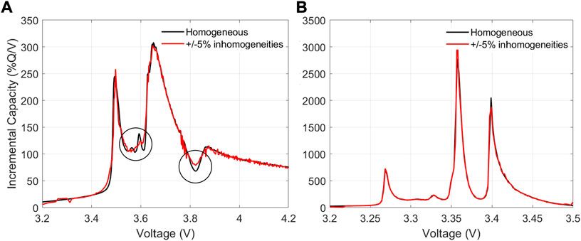
FIGURE 9. Comparison of the voltage response of a homogeneous cell vs. a cell with ±5% of LLI, LAMPE, and LAMNE for (A) a GIC/NMC cell and (B) a GIC/LFP cell.
3 Chemistry-specific comments
3.1 GIC/layered oxide-based batteries (LCO, NCA, and NMCs)
Figure 10A presents the evolution of the IC curves for a GIC/NMC111 cell up to 15% LLI, 10% LAMPE, and 10% LAMNE (full thin line), with 3% increments (dotted lines). For this cell, six peaks can be labeled and seven FOIs can be defined. The intensity of the shoulder at high voltage, ➊★➀, could be used as FOI1 (the area over a small potential range could also be used to average the impact of noise). The intensity and position of the minimum around 3.8 V between ➊★➀ and ➋★➀ could be defined as FOI2 and FOI3, respectively. Finally, the intensity and position of the maximum intensity for peaks ➋★➁ and ➎★➁ can be defined as FOI4 to FOI7, respectively. Peaks ➌★➁ and ➍★➁ are small and cannot be used accurately to track the degradation. Because the half-cell responses of LCO and NMC532 are similar, the FOI definition will be the same for those and will not be repeated. This is also true for NCA, (Figure 10C).
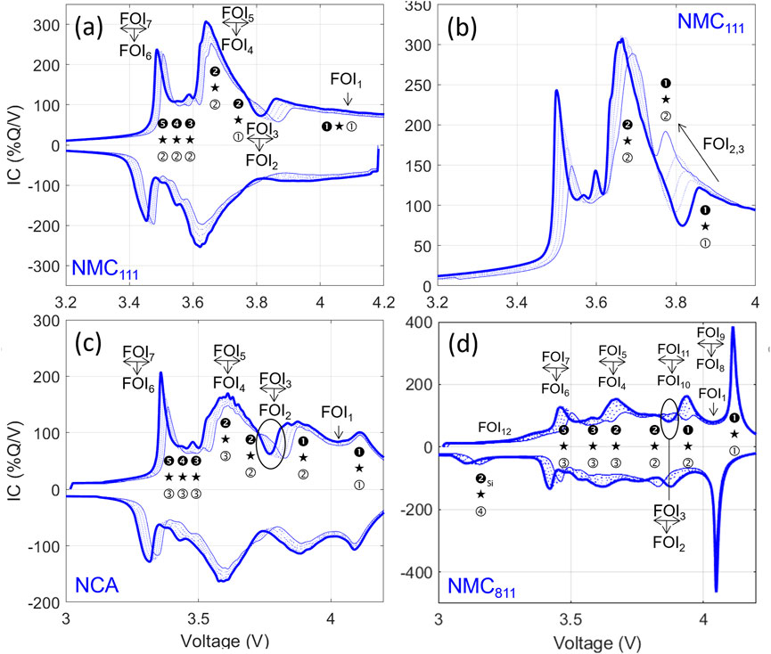
FIGURE 10. Peak evolution from the pristine cell (thick line) to 15% LLI, 10% LAMPE, and 10% LAMGIC (thin line) and intermediates (dotted lines) for (A) GIC/NMC111, (C) GIC/NCA, and (D) (GIC,Si)/NMC811. (B) Effects of NE rate capacity degradation on a GIC/NMC111 cell (C/10 simulation with up to 10% LAMNE with a 4x worsening of the kinetics and an 80% increase of resistance).
Using the degradation map provided in Figure 7, the evolution according to the different degradation modes can be established, Table 1, and this can be used to identify, which FOIs are the most sensitive to specific degradation modes. For these chemistries, LAMPE is easy to determine from FOI1 as long as LAMNE is limited (➊★➀, 4th column). Contrary to what is often found in the literature, the intensity of the main peak ➋★➁ is sensitive to LLI and not LAMPE (2nd column and FOI5). As described earlier, FOI7 is sensitive to LLI and LAMPE (➎★➁, 1st column). LAMNE will be the hardest to quantify from ICA. It could be deciphered from FOI2 after LLI and LAMPE are quantified (➋★➀, 3rd column). If graphitic peaks are well marked, peak area analysis or DVA could be used instead. An example quantification is provided in Section 4. For interested readers, more details can be found in the literature for NMC111 (Carter et al., 2021), NCA (Dubarry et al., 2018a; Dubarry and Beck, 2021), or LCO (Gao et al., 2019; Li et al., 2022).
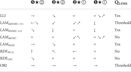
TABLE 1. GIC/NMC111 summary of peak evolution with degradation in charge. Font size is representative of intensity of changes.
Looking at the kinetic aspects, a degradation of the PE kinetics (RDFPE) will sharpen the peaks at low voltages. For degradation of the kinetics of the NE (RDFNE), FOI3 will move toward lower voltages while its intensity (FOI2) is increasing. This induces some counter intuitive peak movements, (Figure 10B). The minimum around 3.8 V corresponds to a staging reaction in graphite. Initially, it occurs during the NMC solid solution. With LAMNE and rate capability degradation, it could occur sooner and sooner and thus against the phase transformation instead of the solid solution. This will result in a new sharp peak, ➊★➁, growing on the IC curves to the detriment of ➋★➀. This peak will move toward lower voltage, while all the others will move toward higher voltages.
The analysis and summary tables for GIC/NMC532, GIC/LCO, and GIC/NCA are similar, with just slight differences in the evolution of some of the peaks. Corresponding look-up tables are presented in Supplementary Table S1–S3, respectively. The full degradation maps are provided in Supplementary Figure S1 for LCO, Supplementary Figure S2 for NMC532, and Supplementary Figure S3 for NCA.
Figure 10D presents the evolution of the IC curves for a (GIC0.9, Si0.1)/NMC811 cell up to 15% LLI, 10% LAMPE, and 10% LAMNE, with the peak indexation. The IC response for this cell is more complex because NMC811 not only has more features but also because of the blending at the NE that add some peaks for Si (➋Si★➃). More details on this cell can be found in Anseán et al. (2020) and Dubarry and Beck (2021). Schmitt et al. also worked extensively on this chemistry (Schmitt et al., 2021; Schmitt et al., 2022). For this system, 12 FOIs can be defined. To be consistent with the previous description, and because their sensibilities are similar, FOIs1–7 were defined identically and their correspondence will not be repeated. FOIs8–11 correspond to the position and intensity of the maximum of the new peaks at 4.1 V (➊★➀) and 3.9 V (➊★➁), respectively. FOI12 corresponds to the new broad peak at low voltage (➋Si★➃). Based on the degradation map, Supplementary Figure S4, and the associated peak displacement table, Supplementary Table S4, FOI1 can still be used to estimate LAMPE. Moreover, the intensity of the high voltage peak ➊★➀ seems really affected by LAMGIC and thus FOI8 can be used for quantification once LAMPE and LLI are quantified. Finally, FOI12 can be used to quantify LAMSi after the other modes are quantified. The intensity and position of the peak at 3.9 V (➊★➁, FOIs10,11) could be used the same way as FOI2 and FOI3 if necessary for LLI or LAMNE quantification.
3.2 Spinel-based batteries (LMO)
LMO-based batteries are getting rarer; nonetheless, LMO is still often used in blended electrodes with NMC (Dubarry et al., 2011b; Smith et al., 2012; Wu and Lee, 2017; Lee et al., 2018; Elliott et al., 2020). Figure 11A presents a summary of the voltage response for a GIC/LMO cell upon aging with peak indexation. Look-up Supplementary Table S5 presents the peak evolution from the associated degradation map, Supplementary Figure S5. For this system, eight FOIs can be defined with the position and intensity of the maximum of the four main peaks. Peaks ➋★➀ and ➋★➁ (FOIs3,4 and FOI5,6) are not well separated but evolved differently depending on the degradation. From the degradation map, it can be seen that LLI is affecting ➊★➀ the most, both in terms of intensity and position. LAMPE is broadening all the peaks significantly while LAMNE is separating ➋★➀ and ➋★➁ by moving ➋★➀ toward higher voltages (FOI3). Looking at the kinetics impact, it is not significant for LMO, which was expected since it is a high-power material. Similarly, to what was observed for the NMCs, a degradation of the kinetics of the NE will broaden the high voltage peaks near the graphite staging.
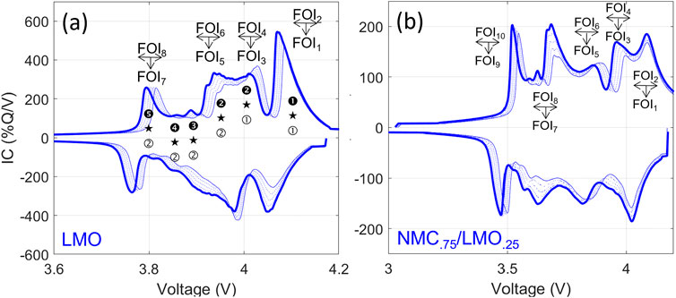
FIGURE 11. Peak evolution from the pristine cell (thick line) to 15% LLI, 10% LAMPE, and 10% LAMNE (thin line) and intermediates (dotted lines) for (A) GIC/LMO and (B) GIC/(NMC.75,LMO.25) cells.
Figure 11B presents the example of a blended PE with 75% of NMC111 and 25% of LMO. Peak indexation was already provided in Figure 3. The peak evolution table is presented in look-up Supplementary Table S6 with the associated degradation map in Supplementary Figure S6. With five main peaks visible on the IC curves, 10 FOIs can be defined. Overall, the observed trends are similar to that of the individual components because the voltage responses are separated (no LMO capacity on the NMC main peak and constant IC intensity from NMC under the LMO peaks). LLI is associated with a lowering of FOI2 and shifting of FOI1 toward higher voltages. Unfortunately, both LAMPEs have a similar signature and might be hard to separate.
3.3 Iron phosphate-based batteries (LFP and LFP + LNO)
The GIC/LFP system was the first one to be really studied using ICA (Dubarry and Liaw, 2009), and it is probably the one with most literature (e.g., (Dubarry et al., 2012; Han et al., 2014; Ouyang et al., 2015)) as it is one of the easiest ICA to carry. The electrochemical response is quite simple, Figure 12A, Supplementary Table S7, and Supplementary Figure S7, with mostly the peaks belonging to the graphite visible but broadened. In terms of FOIs, FOI1 could be defined as the area under the peak ➊★➀ and it is sensitive to LLI and LAMNE. FOI2 could be defined as the area under all the other peaks (➋★➀ to ➎★➀) and it is sensitive to LAMNE. The intensity and position of peak ➎★➀ are mildly sensitive to LAMPE, which could be used as FOI3 and FOI4, respectively (Dubarry et al., 2017; Dubarry and Beck, 2021). The area method is preferred in the case of LFP because the IC intensity almost goes back to zero in-between peaks and because the peaks are sharp, which makes their intensity easily affected by smoothing. The impact of kinetic limitations on LFP was already discussed earlier. An example of analysis for this cell is provided in Section 4.
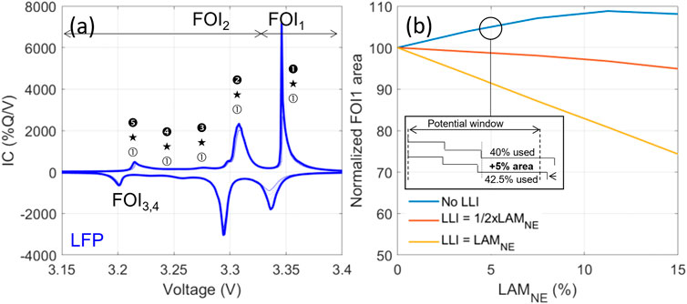
FIGURE 12. (A) Peak evolution from the pristine cell (thick line) to 15% LLI, 10% LAMPE, and 10% LAMNE (thin line) and intermediates (dotted lines) for a GIC/LFP cell. (B) Evolution of FOI for different degradation paths.
While being the most reported, this system is also the one with the most conflictual analyses. This mostly comes from the fact that some authors are considering peak ➊★➀ and FOI1 as sensitive to LLI only and directly proportional to capacity loss. This is not the case as peak ➊★➀ increases with LAMNE while the PE is limiting at EOC, Figure 12B. This counter intuitive effect can be easily explained, inset of Figure 12B. Under normal operation, because of the excess NE, reaction ➊, which accounts for 50% of the graphite capacity, is never completed. Hypothetically, a 10% NE excess in a cell with no offset implies that the cell uses 90% of the graphite capacity and thus only 40% out of the 50% for ➊. If that hypothetical cell lost 5% LAMNE, the cell would not lose any capacity but the excess would be reduced by half. This implies that 95% of the graphite capacity would now be in the potential window and that 45% of ➊ would be used. The area of the peak would therefore be 0.45*0.95, which equals 42.5%, more than the initial 40%. The same effect can be observed when the PE is a blend between LFP and a high-voltage material such as lithium nickel oxide (LNO).
3.4 Lithium titanate-based batteries
Literature using LTO as an NE with IC curves is scarce (Baure et al., 2019; Liu et al., 2019; Baure and Dubarry, 2020; Chahbaz et al., 2021; Ha et al., 2021; Bank et al., 2022), but it presents some interesting cases first because LTO has a completely different voltage response than graphite and because, in most cases, the NE is limiting in charge and discharge.
One of the most common LTO-based batteries is using NMC as the PE but some commercial cells are also using LMO. In addition, our group also studied a cell with a blended PE, containing LCO and NCA in a 1:1 ratio. All these cases are presented in Figure 13, look-up Supplementary Tables S8–S10, and Supplementary Figures S8–S10. For the LTO/NMC cell, four FOIs can be defined with FOI1 being the offset potential at high voltage, FOI2 the shoulder intensity, FOI3 the intensity of peak ➊★➁, and FOI4 its front slope. FOI2 is, just as for the graphite counterpart, sensitive to LAMPE. FOI1 is affected by all modes but a movement toward higher voltages indicates that LLI is preponderant. FOI3 is also going down for LLI but this can be compensated by LAMPE, while FOI4 is neither going up then decreasing (PE limiting at EOD) nor FOI1 going out of the potential window (PE limiting at EOC). Finally, the overall area is directly proportional to LAMNE, Figure 6, unless there was a change in limiting electrodes. Kinetic degradation mostly affects NMC as described previously. LTO is a high-power material so it is not affected much.
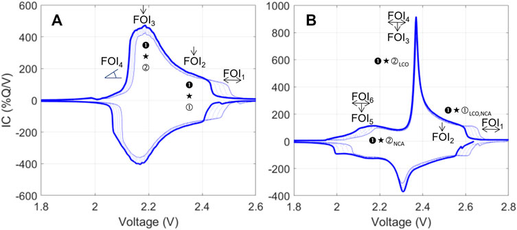
FIGURE 13. (A) Peak evolution from the pristine cell (thick line) to 15% LLI, 10% LAMPE, and 10% LAMNE (thin line) and intermediates (dotted lines) for (A) LTO/NMC and (B) a LTO/(LCO0.5, NCA0.5) cells.
For the LTO/LMO and for LTO/blended electrode, Figure 13B, FOI1 and FOI2 could be defined identically. For the LTO/LMO, the evolution of the peaks is really similar to that of the LTO/NMC cell, and the analysis of the impact of the FOIs is the same. For the blend, because the PE contains two layered oxides, FOI2 is now representative of the total LAMPE. Individual LAMPE could be calculated from FOIs3,4 (intensity/position of peak ➊★➁LCO) for LCO and FOIs5,6 (intensity/position of peak ➊★➁NCA) for NCA.
4 Example of ICA on a GIC/NMC111 and a GIC/LFP cell
Based on the earlier discussion, this section will present a step-by-step analysis of the voltage curves in Figure 10A for a GIC/NMC111 cell and Figure 12A for a GIC/LFP cell.
Starting with Figure 10A and GIC/NMC111 and using Figure 8, the first step is to identify any increase in resistance. Since the plotted data are C/25, changes associated with resistance increase will be really minute. Assuming the discharges all started from the same state of charge, the initial voltage drop can be used to estimate resistance increase. In this example, it decreased by 3 mV, following ohms law, corresponds to an increase of resistance of 75 mΩ.Ah (ΔV/C = 0.003/0.04). The second step is to determine which electrodes are limiting to decipher and which degradation mode is responsible for the capacity loss (15.6%). Since peak ➎★➁ moved toward higher voltages, and since no plating is visible at high voltage, it can be determined that LLI is solely responsible for the capacity loss. Using the equation in Figure 6 and assuming a 5% offset, LLI can be quantified at around 14.8%. Following on, using Figure 7 and Table 1, the next degradation mode to quantify should be LAMPE as it is directly obtainable from FOI1. At 4 V, the initial IC intensity is of 88.6 %Q/V and of 80.2 %Q/V for the final aged curve, a 9.1% difference. This corresponds to LAMPE. For a proper estimation of LAMNE using the IC curves, the correct procedure would be to simulate the voltage response associated with 14.8% LLI and 9.1% LAMPE with different amount of LAMNE until a satisfactory match is reached. If no model is available, and since the graphitic transition from ➋ to ➊ (FOI2) is well visible for all curves, the peak area method could provide an estimate for LAMNE. The area from the start of the charge to the local minimum around 3.8 V decreased by linearly by 9.6%. Another option could be to use the DV curves (not shown). Doing so will show that the distance between the two main graphite peaks decreased from 39.3% to 35.3%, thus by 10.2%. Overall, the obtained values are close to the 15% LLI, 10% LAMPE, and 10% LAMNE used for the simulations.
Taking a GIC//LFP cell as the second example, Figure 12A and using the same logic, it can be determined that no significant resistance increase was visible and that the capacity loss (17%) was also induced by LLI. Assuming an offset of around 10%, LLI can be estimated to be around 15.3% using the equation provided in Figure 6. In order to estimate LAMNE, FOI2, and the evolution of the area under peaks ➋★➀ to ➎★➀ can be used. FOI2 varied by 10%, which corresponds to LAMNE. FOI1 varied by 20% instead of the predicted 38% based solely on LLI because it was increased by LAMNE as explained earlier, (Figure 12B). Small LAMPE are almost impossible to quantify on GIC/LFP cells without the use of a model to simulate and separate the small peak variations induced by the LLI and LAMNE. Nonetheless, since peak ➎★➁ is still visible, and since its area only varied by 11%, as expected from the LAMNE, it can be determined that LAMPE is significantly lower than 20% (LLI + offset).
5 Conclusion
The incremental capacity analysis has proven to be an effective and versatile technique for in situ diagnosis of Li-ion batteries. This publication presented best practices with detailed examples for the majority of the battery chemistry available to date. Key takeaways to facilitate its application are summarized in Table 2.
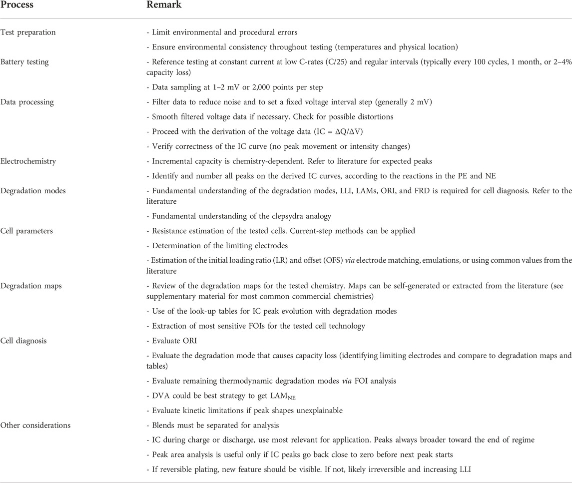
TABLE 2. Best practices for incremental capacity analysis.
Looking further, and toward more accurate on-board applications, methodological work is still needed to better enable operando analysis at high rates and for duty cycles outside of constant current. This would remove the need for lengthy maintenance cycles. Moreover, quantification of the impact of inhomogeneities is also needed to analyze the changes in the electrochemical response for large single cells and battery packs. More discussion of these topics can be found in Dubarry and Beck (2022).
Data availability statement
The datasets presented in this study can be found in online repositories. The names of the repository/repositories and accession numbers can be found at: 10.17632/4k8f4t352y.1.
Author contributions
MD: initial draft and editing. DA: review, table preparation, and editing.
Funding
MD was funded by the Office of Naval Research (ONR), grant number N00014-19-1-2159. DA gratefully acknowledges the funding provided by the Spanish Ministry of Science and Innovation and by FEDER funds via Project MCI-20-PID2019-110955RB-I00 and the José Castillejo mobility grants via CAS21/00034.
Acknowledgments
MD is extremely grateful to Joel Gaubicher (IMN, France), Dominique Guyomard (IMN, France), and Yves Chabre for teaching him be the basics on IC and to all the former students who helped to develop the methodology, especially Cyril Truchot (APPLE, United States), David Anseán (University of Oviedo, Spain), and Arnaud Devie (Element Energy, United States). MD is also thankful to Alexa Fernando, David Beck (HNEI, United States), Yuliya Preger, Reed Wittman (SANDIA, United States), Andrew Weng (University of Michigan, United States), and Alejandro Gismero (Aalborg University, Denmark) for fruitful discussions and comments while writing this publication.
Conflict of interest
The authors declare that the research was conducted in the absence of any commercial or financial relationships that could be construed as a potential conflict of interest.
Publisher’s note
All claims expressed in this article are solely those of the authors and do not necessarily represent those of their affiliated organizations, or those of the publisher, the editors, and the reviewers. Any product that may be evaluated in this article, or claim that may be made by its manufacturer, is not guaranteed or endorsed by the publisher.
Supplementary material
The Supplementary Material for this article can be found online at: https://www.frontiersin.org/articles/10.3389/fenrg.2022.1023555/full#supplementary-material
Abbreviations
BOL, beginning of life; DV, differential voltage; DVA, differential voltage analysis; EOC, end of charge; EOD, end of discharge; FOI, feature of interest; FRD, faradic rate degradation; GIC, graphite intercalation compound; IC, incremental capacity; ICA, incremental capacity analysis; KL, kinetic limitations; LAM, loss of active material; LFP, lithium iron phosphate; LCO, lithium cobalt oxide; LLI, loss of lithium inventory; LMO, lithium manganese oxide; LNO, lithium nickel oxide; LR, loading ratio; LTO, lithium titanium oxide; NCA, nickel cobalt aluminum oxide; NMC, nickel manganese cobalt oxide; PE, positive electrode; NE, negative electrode; OFS, offset; ORI, ohmic resistance increase; Q, capacity; RDF, rate degradation factor; SEI, solid electrolyte interphase; and V, voltage.
References
Anseán, D., Baure, G., González, M., Cameán, I., García, A. B., and Dubarry, M. (2020). Mechanistic investigation of silicon-graphite/LiNi0.8Mn0.1Co0.1O2 commercial cells for non-intrusive diagnosis and prognosis. J. Power Sources 459, 227882. doi:10.1016/j.jpowsour.2020.227882
Anseán, D., Dubarry, M., Devie, A., Liaw, B. Y., García, V. M., Viera, J. C., et al. (2016). Fast charging technique for high power LiFePO4 batteries: A mechanistic analysis of aging. J. Power Sources 321, 201–209. doi:10.1016/j.jpowsour.2016.04.140
Anseán, D., Dubarry, M., Devie, A., Liaw, B. Y., García, V. M., Viera, J. C., et al. (2017). Operando lithium plating quantification and early detection of a commercial LiFePO 4 cell cycled under dynamic driving schedule. J. Power Sources 356, 36–46. doi:10.1016/j.jpowsour.2017.04.072
Attia, P. M., Bills, A. A., Brosa Planella, F., Dechent, P., dos Reis, G., Dubarry, M., et al. (2022). Review—"Knees" in lithium-ion battery aging trajectories. J. Electrochem. Soc. 169, 060517. doi:10.1149/1945-7111/ac6d13
Balewski, L., and Brenet, J. P. (1967). A new method for the study of the electrochemical reactivity of manganese dioxide. Electrochem. Technol. 5 (11-12), 527–531.
Bank, T., Alsheimer, L., Löffler, N., and Sauer, D. U. (2022). State of charge dependent degradation effects of lithium titanate oxide batteries at elevated temperatures: An in-situ and ex-situ analysis. J. Energy Storage 51, 104201. doi:10.1016/j.est.2022.104201
Barai, A., Uddin, K., Dubarry, M., Somerville, L., McGordon, A., Jennings, P., et al. (2019). A comparison of methodologies for the non-invasive characterisation of commercial Li-ion cells. Prog. Energy Combust. Sci. 72, 1–31. doi:10.1016/j.pecs.2019.01.001
Barker, J. (1989). An Electrochemical Investigation of the doping processes in poly(thienylene vinylene). Synth. Met. 33, 43–50. doi:10.1016/0379-6779(89)90828-x
Barker, J., Saidi, M. Y., and Swoyer, J. L. (2003b). A sodium-ion cell based on the fluorophosphate compound NaVPO[sub 4]F. Electrochem. Solid-State Lett. 6 (1), A1. doi:10.1149/1.1523691
Barker, J., Saidi, M. Y., and Swoyer, J. L. (2003a). Performance evaluation of the electroactive material, γ-LiV[sub 2]O[sub 5], made by a carbothermal reduction method. J. Electrochem. Soc. 150 (9), A1267. doi:10.1149/1.1600462
Baure, G., Devie, A., and Dubarry, M. (2019). Battery durability and reliability under electric utility grid operations: Path dependence of battery degradation. J. Electrochem. Soc. 166 (10), A1991–A2001. doi:10.1149/2.0971910jes
Baure, G., and Dubarry, M. (2020). Battery durability and reliability under electric utility grid operations: 20-year forecast under different grid applications. J. Energy Storage 29, 101391. doi:10.1016/j.est.2020.101391
Baure, G., and Dubarry, M. (2019). Synthetic vs. Real driving cycles: A comparison of electric vehicle battery degradation. Batteries 5 (2), 42. doi:10.3390/batteries5020042
Birkl, C. R., Roberts, M. R., McTurk, E., Bruce, P. G., and Howey, D. A. (2017). Degradation diagnostics for lithium ion cells. J. Power Sources 341, 373–386. doi:10.1016/j.jpowsour.2016.12.011
Bloom, I., Jansen, A. N., Abraham, D. P., Knuth, J., Jones, S. A., Battaglia, V. S., et al. (2005). Differential voltage analyses of high-power, lithium-ion cells: 1. Technique and application. J. Power Sources 139 (1–2), 295 –303. doi:10.1016/j.jpowsour.2004.07.021
Carter, R., Kingston, T. A., Atkinson, R. W., Parmananda, M., Dubarry, M., Fear, C., et al. (2021). Directionality of thermal gradients in lithium-ion batteries dictates diverging degradation modes. Cell Rep. Phys. Sci. 2, 100351. doi:10.1016/j.xcrp.2021.100351
Chahbaz, A., Meishner, F., Li, W., Ünlübayirl, C., and Uwe Sauer, D. (2021). Non-invasive identification of calendar and cyclic ageing mechanisms for lithium-titanate-oxide batteries. Energy Storage Mater. 42, 794–805. doi:10.1016/j.ensm.2021.08.025
Chen, Y., Torres-Castro, L., Chen, K.-H., Penley, D., Lamb, J., Karulkar, M., et al. (2022). Operando detection of Li plating during fast charging of Li-ion batteries using incremental capacity analysis. J. Power Sources 539, 231601. doi:10.1016/j.jpowsour.2022.231601
Dahn, J., and Haering, R. R. (1981). The role of kinetic effects in voltammetry studies of intercalation systems. Solid State Ionics 2, 19–26. doi:10.1016/0167-2738(81)90014-x
Devie, A., and Dubarry, M. (2016). Durability and reliability of electric vehicle batteries under electric utility grid operations. Part 1: Cell-to-Cell variations and preliminary testing. Batteries 2 (3), 28. doi:10.3390/batteries2030028
Devie, A., Dubarry, M., Wu, H.-P., Wu, T.-H., and Liaw, B. Y. (2016). Overcharge study in Li4Ti5O12 based lithium-ion pouch cell, II. Experimental investigation of the degradation mechanism. J. Electrochem. Soc. 163 (13), A2611–A2617. doi:10.1149/2.0491613jes
Dubarry, M., and Anseán González, D. (2022). Synthetic data for Li-ion batteries degradation maps with degradation example. Mendeley Data. 1. doi:10.17632/4k8f4t352y.1
Dubarry, M., Baure, G., and Anseán, D. (2020). Perspective on state-of-health determination in lithium-ion batteries. J. Electrochem. Energy Convers. Storage 17 (4), 1–25. doi:10.1115/1.4045008
Dubarry, M., Baure, G., and Devie, A. (2018a). Durability and reliability of EV batteries under electric utility grid operations: Path dependence of battery degradation. J. Electrochem. Soc. 165 (5), A773–A783. doi:10.1149/2.0421805jes
Dubarry, M., Baure, G., Pastor-Fernández, C., Yu, T. F., Widanage, W. D., and Marco, J. (2019). Battery energy storage system modeling: A combined comprehensive approach. J. Energy Storage 21, 172–185. doi:10.1016/j.est.2018.11.012
Dubarry, M., and Baure, G. (2020). Perspective on commercial Li-ion battery testing, best practices for simple and effective protocols. Electronics 9 (1), 152. doi:10.3390/electronics9010152
Dubarry, M., and Beck, D. (2021). Analysis of synthetic voltage vs. Capacity datasets for big data Li-ion diagnosis and prognosis. Energies 14 (9), 2371. doi:10.3390/en14092371
Dubarry, M., and Beck, D. (2022). Perspective on mechanistic modeling of Li-ion batteries. Acc. Mat. Res. 3 (8), 843–853. doi:10.1021/accountsmr.2c00082
Dubarry, M., Berecibar, M., Devie, A., Anseán, D., Omar, N., and Villarreal, I. (2017). State of health battery estimator enabling degradation diagnosis: Model and algorithm description. J. Power Sources 360, 59–69. doi:10.1016/j.jpowsour.2017.05.121
Dubarry, M., Gaubicher, J., Guyomard, D., Wallez, G., Quarton, M., and Baehtz, C. (2008). Uncommon potential hysteresis in the Li/Li2xVO(H2−xPO4)2 (0≤x≤2) system. Electrochimica Acta 53 (13), 4564–4572. doi:10.1016/j.electacta.2007.12.085
Dubarry, M., and Liaw, B. Y. (2009). Identify capacity fading mechanism in a commercial LiFePO4 cell. J. Power Sources 194 (1), 541–549. doi:10.1016/j.jpowsour.2009.05.036
Dubarry, M., Qin, N., and Brooker, P. (2018b). Calendar aging of commercial Li-ion cells of different chemistries – a review. Curr. Opin. Electrochem. 9, 106–113. doi:10.1016/j.coelec.2018.05.023
Dubarry, M., Svoboda, V., Hwu, R., and Yann Liaw, B. (2006). Incremental capacity analysis and close-to-equilibrium OCV measurements to quantify capacity fade in commercial rechargeable lithium batteries. Electrochem. Solid-State Lett. 9 (10), A454–A457. doi:10.1149/1.2221767
Dubarry, M., Truchot, C., Cugnet, M., Liaw, B. Y., Gering, K., Sazhin, S., et al. (2011a). Evaluation of commercial lithium-ion cells based on composite positive electrode for plug-in hybrid electric vehicle applications. Part I: Initial characterizations. J. Power Sources 196 (23), 10328–10335. doi:10.1016/j.jpowsour.2011.08.077
Dubarry, M., Truchot, C., Devie, A., Liaw, B. Y., Gering, K., Sazhin, S., et al. (2015). Evaluation of commercial lithium-ion cells based on composite positive electrode for plug-in hybrid electric vehicle (PHEV) applications. J. Electrochem. Soc. 162 (9), A1787–A1792. doi:10.1149/2.0481509jes
Dubarry, M., Truchot, C., and Liaw, B. Y. (2014). Cell degradation in commercial LiFePO4 cells with high-power and high-energy designs. J. Power Sources 258, 408–419. doi:10.1016/j.jpowsour.2014.02.052
Dubarry, M., Truchot, C., Liaw, B. Y., Gering, K., Sazhin, S., Jamison, D., et al. (2013). Evaluation of commercial lithium-ion cells based on composite positive electrode for plug-in hybrid electric vehicle applications. J. Electrochem. Soc. 160 (1), A191–A199. doi:10.1149/2.063301jes
Dubarry, M., Truchot, C., Liaw, B. Y., Gering, K., Sazhin, S., Jamison, D., et al. (2011b). Evaluation of commercial lithium-ion cells based on composite positive electrode for plug-in hybrid electric vehicle applications. Part II. Degradation mechanism under 2C cycle aging. J. Power Sources 196 (23), 10336–10343. doi:10.1016/j.jpowsour.2011.08.078
Dubarry, M., Truchot, C., and Liaw, B. Y. (2012). Synthesize battery degradation modes via a diagnostic and prognostic model. J. Power Sources 219, 204–216. doi:10.1016/j.jpowsour.2012.07.016
Dubarry, M., Vuillaume, N., and Liaw, B. Y. (2009). From single cell model to battery pack simulation for Li-ion batteries. J. Power Sources 186 (2), 500–507. doi:10.1016/j.jpowsour.2008.10.051
Elliott, M., Swan, L. G., Dubarry, M., and Baure, G. (2020). Degradation of electric vehicle lithium-ion batteries in electricity grid services. J. Energy Storage 32, 101873. doi:10.1016/j.est.2020.101873
Fath, J. P., Dragicevic, D., Bittel, L., Nuhic, A., Sieg, J., Hahn, S., et al. (2019). Quantification of aging mechanisms and inhomogeneity in cycled lithium-ion cells by differential voltage analysis. J. Energy Storage 25, 100813. doi:10.1016/j.est.2019.100813
Feng, X., Li, J., Ouyang, M., Lu, L., Li, J., and He, X. (2013). Using probability density function to evaluate the state of health of lithium-ion batteries. J. Power Sources 232, 209–218. doi:10.1016/j.jpowsour.2013.01.018
Feng, X., Merla, Y., Weng, C., Ouyang, M., He, X., Liaw, B. Y., et al. (2020). A reliable approach of differentiating discrete sampled-data for battery diagnosis. eTransportation 3, 100051. doi:10.1016/j.etran.2020.100051
Fly, A., Wimarshana, B., Bin-Mat-Arishad, I., and Sarmiento-Carnevali, M. (2022). Temperature dependency of diagnostic methods in lithium-ion batteries. J. Energy Storage 52, 104721. doi:10.1016/j.est.2022.104721
Gao, Y., Yang, S., Jiang, J., Zhang, C., Zhang, W., and Zhou, X. (2019). The mechanism and characterization of accelerated capacity deterioration for lithium-ion battery with Li(NiMnCo) O2 cathode. J. Electrochem. Soc. 166 (8), A1623–A1635. doi:10.1149/2.1001908jes
Gauthier, R., Luscombe, A., Bond, T., Bauer, M., Johnson, M., Harlow, J., et al. (2022). How do depth of discharge, C-rate and calendar age affect capacity retention, impedance growth, the electrodes, and the electrolyte in Li-ion cells? J. Electrochem. Soc. 169, 2. doi:10.1149/1945-7111/ac4b82
Ha, Y., Harvey, S. P., Teeter, G., Colclasure, A. M., Trask, S. E., Jansen, A. N., et al. (2021). Long-term cyclability of Li4Ti5O12/LiMn2O4 cells using carbonate-based electrolytes for behind-the-meter storage applications. Energy Storage Mater. 38, 581–589. doi:10.1016/j.ensm.2021.03.036
Han, X., Ouyang, M., Lu, L., Li, J., Zheng, Y., and Li, Z. (2014). A comparative study of commercial lithium ion battery cycle life in electrical vehicle: Aging mechanism identification. J. Power Sources 251, 38–54. doi:10.1016/j.jpowsour.2013.11.029
Huggins, R. (2016). Energy storage fundamentals materials and applications. 2nd edition. United States: Springer International Publishing.
Khodr, Z., Mallet, C., Daigle, J.-C., Feng, Z., Amouzegar, K., Claverie, J., et al. (2020). Electrochemical study of functional additives for Li-ion batteries. J. Electrochem. Soc. 167 (12), 120535. doi:10.1149/1945-7111/abae92
Lee, P.-H., Wu, S.-h., Pang, W. K., and Peterson, V. K. (2018). The storage degradation of an 18650 commercial cell studied using neutron powder diffraction. J. Power Sources 374, 31–39. doi:10.1016/j.jpowsour.2017.11.021
Lewerenz, M., and Sauer, D. U. (2018). Evaluation of cyclic aging tests of prismatic automotive LiNiMnCoO2-Graphite cells considering influence of homogeneity and anode overhang. J. Energy Storage 18, 421–434. doi:10.1016/j.est.2018.06.003
Li, S., Tsutsumi, S., Shironita, S., and Umeda, M. (2022). Verification of peak attribution in differential capacity profile by varying the electrode capacity balance in three-electrode Li-ion laminate cells. Electrochemistry 90 (6), 067004. doi:10.5796/electrochemistry.22-00036
Li, Y., Abdel-Monem, M., Gopalakrishnan, R., Berecibar, M., Nanini-Maury, E., Omar, N., et al. (2018). A quick on-line state of health estimation method for Li-ion battery with incremental capacity curves processed by Gaussian filter. J. Power Sources 373, 40–53. doi:10.1016/j.jpowsour.2017.10.092
Liu, P., Wu, Y., She, C., Wang, Z., and Zhang, Z. (2022). Comparative study of incremental capacity curve determination methods for lithium-ion batteries considering the real-world situation. IEEE Trans. Power Electron. 37 (10), 12563–12576. doi:10.1109/tpel.2022.3173464
Liu, S., Winter, M., Lewerenz, M., Becker, J., Sauer, D. U., Ma, Z., et al. (2019). Analysis of cyclic aging performance of commercial Li4Ti5O12-based batteries at room temperature. Energy 173, 1041–1053. doi:10.1016/j.energy.2019.02.150
MacNeil, D. D., Lu, Z., and Dahn, J. R. (2002). Structure and Electrochemistry of Li[Ni[sub x]Co[sub 1−2x]Mn[sub x]]O[sub 2] (0≤x≤1/2). J. Electrochem. Soc. 149 (10), A1332–A1336. doi:10.1149/1.1505633
Noh, H.-J., Youn, S., Yoon, C. S., and Sun, Y.-K. (2013). Comparison of the structural and electrochemical properties of layered Li[NixCoyMnz]O2 (x = 1/3, 0.5, 0.6, 0.7, 0.8 and 0.85) cathode material for lithium-ion batteries. J. Power Sources 233, 121–130. doi:10.1016/j.jpowsour.2013.01.063
Ouyang, M., Chu, Z., Lu, L., Li, J., Han, X., Feng, X., et al. (2015). Low temperature aging mechanism identification and lithium deposition in a large format lithium iron phosphate battery for different charge profiles. J. Power Sources 286, 309–320. doi:10.1016/j.jpowsour.2015.03.178
Ratnakumar, B. V., and Smart, M. C. (2010). Lithium plating behavior in lithium-ion cells. ECS Trans. 25 (36), 241–252. doi:10.1149/1.3393860
Reimers, J., and Dahn, J. R. (1992). Electrochemical and in situ X-ray diffraction studies of lithium intercalation in LixCoO2. J. Electrochem. Soc. 138 (8), 2091–2097. doi:10.1149/1.2221184
Rodrigues, M.-T. F., Gim, J., Tornheim, A., Kahvecioglu, O., Luo, M., Prado, A. Y. R., et al. (2022). Concealed cathode degradation in lithium-ion cells with a Ni-rich oxide. J. Electrochem. Soc. 169 (4), 040539. doi:10.1149/1945-7111/ac65b7
Schindler, S., Baure, G., Danzer, M. A., and Dubarry, M. (2019). Kinetics accommodation in Li-ion mechanistic modeling. J. Power Sources 440, 227117. doi:10.1016/j.jpowsour.2019.227117
Schmidt, J. P., Tran, H. Y., Richter, J., Ivers-Tiffée, E., and Wohlfahrt-Mehrens, M. (2013). Analysis and prediction of the open circuit potential of lithium-ion cells. J. Power Sources 239, 696–704. doi:10.1016/j.jpowsour.2012.11.101
Schmitt, J., Schindler, M., and Jossen, A. (2021). Change in the half-cell open-circuit potential curves of silicon–graphite and nickel-rich lithium nickel manganese cobalt oxide during cycle aging. J. Power Sources 506, 230240. doi:10.1016/j.jpowsour.2021.230240
Schmitt, J., Schindler, M., Oberbauer, A., and Jossen, A. (2022). Determination of degradation modes of lithium-ion batteries considering aging-induced changes in the half-cell open-circuit potential curve of silicon–graphite. J. Power Sources 532, 231296. doi:10.1016/j.jpowsour.2022.231296
Shim, J., Kostecki, R., Richardson, T., Song, X., and Striebel, K. A. (2002). Electrochemical analysis for cycle performance and capacity fading of a lithium-ion battery cycled at elevated temperature. J. Power Sources 112 (1), 222–230. doi:10.1016/s0378-7753(02)00363-4
Shim, J., and Striebel, K. A. (2003a). Characterization of high-power lithium-ion cells during constant current cycling. J. Power Sources 122 (2), 188–194. doi:10.1016/s0378-7753(03)00351-3
Shim, J., and Striebel, K. A. (2003b). Cycling performance of low-cost lithium ion batteries with natural graphite and LiFePO4. J. Power Sources 119-121, 955–958. doi:10.1016/s0378-7753(03)00297-0
Shim, J., and Striebel, K. A. (2004). The dependence of natural graphite anode performance on electrode density. J. Power Sources 130 (1-2), 247–253. doi:10.1016/j.jpowsour.2003.12.015
Sieg, J., Storch, M., Fath, J., Nuhic, A., Bandlow, J., Spier, B., et al. (2020). Local degradation and differential voltage analysis of aged lithium-ion pouch cells. J. Energy Storage 30, 101582. doi:10.1016/j.est.2020.101582
Smith, A. J., Smith, S. R., Byrne, T., Burns, J. C., and Dahn, J. R. (2012). Synergies in blended LiMn2O4 and Li[Ni1/3Mn1/3Co1/3]O2 positive electrodes. J. Electrochem. Soc. 159 (10), A1696–A1701. doi:10.1149/2.056210jes
Striebel, K., Guerfi, A., Shim, J., Armand, M., Gauthier, M., and Zaghib, K. (2003). LiFePO4/gel/natural graphite cells for the BATT program. J. Power Sources 119-121, 951–954. doi:10.1016/s0378-7753(03)00295-7
Tanim, T. R., Dufek, E. J., and Sazhin, S. V. (2021). Challenges and needs for system-level electrochemical lithium-ion battery management and diagnostics. MRS Bull. 46 (5), 420–428. doi:10.1557/s43577-021-00101-8
Tanim, T. R., Shirk, M. G., Bewley, R. L., Dufek, E. J., and Liaw, B. Y. (2018). Fast charge implications: Pack and cell analysis and comparison. J. Power Sources 381, 56–65. doi:10.1016/j.jpowsour.2018.01.091
von Kolzenberg, L., Stadler, J., Fath, J., Ecker, M., Horstmann, B., and Latz, A. (2022). A four parameter model for the solid-electrolyte interphase to predict battery aging during operation. J. Power Sources 539, 231560. doi:10.1016/j.jpowsour.2022.231560
Waldmann, T., Iturrondobeitia, A., Kasper, M., Ghanbari, N., Aguesse, F., Bekaert, E., et al. (2016). Review—post-mortem analysis of aged lithium-ion batteries: Disassembly methodology and physico-chemical analysis techniques. J. Electrochem. Soc. 163 (10), A2149–A2164. doi:10.1149/2.1211609jes
Weng, A., Mohtat, P., Attia, P. M., Sulzer, V., Lee, S., Less, G., et al. (2021). Predicting the impact of formation protocols on battery lifetime immediately after manufacturing. Joule 5, 2971–2992. doi:10.1016/j.joule.2021.09.015
Wu, S.-h., and Lee, P.-H. (2017). Storage fading of a commercial 18650 cell comprised with NMC/LMO cathode and graphite anode. J. Power Sources 349, 27–36. doi:10.1016/j.jpowsour.2017.03.002
Xu, K. (2022). Navigating the minefield of battery literature. Commun. Mat. 3 (1), 31. doi:10.1038/s43246-022-00251-5
Keywords: incremental capacity (IC or dQ/dV), ICA, Li-ion, voltage response, degradation modes
Citation: Dubarry M and Anseán D (2022) Best practices for incremental capacity analysis. Front. Energy Res. 10:1023555. doi: 10.3389/fenrg.2022.1023555
Received: 19 August 2022; Accepted: 08 September 2022;
Published: 03 October 2022.
Edited by:
Tal Sholklapper, Voltaiq, United StatesReviewed by:
Laisuo Su, University of Texas at Austin, United StatesHaifeng Dai, Tongji University, China
Copyright © 2022 Dubarry and Anseán. This is an open-access article distributed under the terms of the Creative Commons Attribution License (CC BY). The use, distribution or reproduction in other forums is permitted, provided the original author(s) and the copyright owner(s) are credited and that the original publication in this journal is cited, in accordance with accepted academic practice. No use, distribution or reproduction is permitted which does not comply with these terms.
*Correspondence: Matthieu Dubarry, bWF0dGhpZXVAaGF3YWlpLmVkdQ==