A complex grid investment decision method considering source-grid-load-storage integration

With the widespread use of renewable energy worldwide, the impact of its randomness and volatility on the grid is increasing. To promote the consumption of renewable energy, the traditional grid is being transformed into a complex grid with integrated source–grid–load–storage. Since the complex grid has the characteristics of source–grid–load–storage interaction, the traditional grid investment decision method will no longer be applicable. First, this study proposes the unilateral indexes of source, grid, load, and storage in complex grids and the interactive indexes considering grid–source interaction, load–grid interaction, source–load interaction, source–storage interaction, load–storage interaction, and grid–storage interaction are proposed to establish the investment decision system. Then, a hesitance fuzzy linguistic term set combined with regret theory is used to calculate the specific values of the subjectivity index, taking into full consideration the regret avoidance and loss avoidance psychology of investors. In order to comprehensively consider the index preference of investors and the objectivity of weight assignment, a combined weighting method based on the analytic network process (ANP) and entropy weight method (EWM) is obtained according to the game theory method. Finally, using a grid in a region of southwest China as an example, the results demonstrate that the construction order obtained in this study can prioritize the projects with the largest comprehensive benefits while considering the subjective preferences of decision-makers and the objectivity of the indexes.

1 Introduction

In recent years, with the rapid growth of the world economy and progress of the society, energy consumption is increasing. Although governments have strongly supported the use of renewable energy recently, traditional fossil energy still dominates the global energy structure. For example, data from the National Energy Administration indicate that the proportion of coal in China’s energy composition reaches 56% (NEA, 2022), which greatly exceeds the proportion of other energy sources. The large amount of greenhouse gases emitted by the large-scale use of coal puts a huge pressure on the environment. New energy sources such as wind power and photovoltaics have the advantages of low pollution, large reserves, renewable, and low pressure on the environment (Mohtasham, 2015), making them the primary choice for solving today’s serious environmental pollution and resource depletion problems. However, with the widespread use of new energy sources, their randomness, volatility, and uncertainty (Li et al., 2019) add modulation difficulties and operational risks to the need for safe and stable operation of power grids, which restricts the development and utilization of renewable energy sources to a certain degree and also cause difficulties in grid connection. Electrochemical energy storage (Zhang, 2013) and flexible load (Chen et al., 2018) can achieve a balance between electricity production and consumption which is why they are widely used in grids containing large amounts of renewable energy. With the rise of renewable energy, flexible load, and electrochemical energy storage in traditional power grids, their degree of grid–source, load–grid, source–load, source–storage, load–storage, and grid–storage interaction is deepening and their integration is strengthening, forming a complex grid with source–grid–load–storage integration. The construction of a safe, stable, economical, and efficient complex grid has become an urgent need for investors (Liu et al., 2016).

Since the traditional grid investment decision method focuses mainly on the unilateral indexes of source–grid–load–storage, the coupling influence between source–grid–load–storage is not considered comprehensively, and its investment decision may have inaccurate results. For example, electrochemical energy storage and grid interaction can regulate peak and frequency (Dasgupta et al., 2015), reduce grid-side grid loss and the amount of heavy load line, improve its network coordination, and thus achieve the purpose of slowing down the construction of new lines. The construction of flexible load near power sources can promote the local consumption of new energy (Yang et al., 2021), which can play a role in reducing the pressure of new energy outgoing and thus slow down the construction of new lines. In the interaction between electrochemical energy storage and flexible load and power supply, both can play a role in reducing abandoned wind and solar power and maintaining the power balance of the grid, so electrochemical energy storage and flexible load will also influence the construction order of each other. Due to the aforementioned reasons, the traditional investment decision method is difficult to meet the complex grid construction needs under the source–grid–load–storage integration conditions, and a new investment decision method is urgently needed.

The main contributions of this study are as follows: 1) an investment decision index system that takes into account the interaction of each side of the complex grid is established, which can comprehensively evaluate the safety, technicality, and economy of each part of the source–grid–load–storage. 2) An EWM–ANP combination weighting method based on game theory is established, considering the interaction and feedback relationship of each part of the complex grid, and the subjective preferences of decision makers and the objectivity of the indexes are fully considered. 3) A subjective index calculation method based on hesitation and regret theory is obtained, taking into account the hesitation and regret psychology of decision makers. The subjective index calculation method based on hesitation linguistic fuzzy term set-regret theory is obtained by accounting for the hesitation and regret psychology of decision makers.

Our study analyzed a total of 16 projects to be built on each side of the source–grid–load–storage in an actual grid in a region of southwest China, and the construction order of the projects to be built on each side of the complex grid is derived using the distance vector merging algorithm (Wang et al., 2019). Our results emphasize that 1) the method in this study comprehensively considers technical, economic, and safety perspectives, and not the better economic projects are built first. 2) The weights in this study consider the different interaction and feedback relationships of each side of source–grid–load–storage, so the weights of each side are different.

2 Literature review

The power system investment decision method mainly focuses on the establishment of the index system and the research with the weighting method. For the establishment of the index system, the Zhang et al. (2021a) constructed the distributed generation source investment decision system from economic benefits and environmental benefits. (Şengül et al., 2015; Koponen and le Net, 2021) constructed the renewable energy investment decision index system from technology, economy, environment, and society. (Ma et al., 2019; Wang et al., 2019; Qian et al., 2022) established a comprehensive decision system for grid investment from technical benefit, economic benefit, and social benefit. Zhang et al. (2021b) established a comprehensive decision system for multi-energy systems from the investment cost of the distribution grid, renewable energy, and electrochemical energy storage equipment. Li et al. (2021) evaluated the effect of flexible load participation in grid interaction from interaction participation, interaction effect, and grid security. Han et al. (2016) established an economic decision method for coupled photovoltaic-storage-microgrid systems based on cost–benefit analysis with the objective of the maximum life-cycle net profit.

In the study of weighting methods, there are methods such as the analysis hierarchical process (Gao et al., 2021), analytic network process (Xiao et al., 2004), Delphi method (Zeng et al., 2016), principal component analysis (Liu et al., 2015), entropy weight method (Kao and van Roy, 2014), anti-entropy weight method (Liu et al., 2019), gray relational analysis (Xiang et al., 2019), coefficient of variation method (Zhang et al., 2018), and the combination methods of the aforementioned methods for weighting (Zhu and Zhang, 2019). In the analysis hierarchical process (AHP), the indexes are independent of each other, which is not applicable for assigning weight investment decisions with interactions in a complex grid. The analytic network process has a very complex computational process. The Delphi method is time-consuming. The principal component analysis method needs to ensure that several principal components extracted have an actual background and meaningful interpretation. The entropy weight method, anti-entropy weight method, and the coefficient of variation method generally have the disadvantage that the subjective preferences of decision makers are not taken into account and the weights change with the modeled samples. Gray relational analysis requires a large amount of data, and the data should follow a typical distribution of some mathematical statistics.

To solve the aforementioned issues, an investment decision system that takes into account the source–grid–load–storage interaction of a complex grid was established in this study. In order to consider the hesitation and regret psychology of experts, hesitance fuzzy linguistic term sets combined with regret theory were used to calculate the qualitative index. In order to consider the dependency and feedback relationship of source–grid–load–storage indexes and overcome the shortage of the subjective assignment method, a combined weighting method based on the game theory of the analytic network process and entropy weight method was proposed so that the assigned weights have the advantage of expert experience and avoid the subjective arbitrariness of assignment. It can be observed from the results of the algorithm (Ma et al., 2019) that the method can provide decision-making support for complex grid investments.

However, to our knowledge, there are few index systems that comprehensively consider the interactions between source–grid–load–storage and can simultaneously evaluate projects on each side of the source–grid–load–storage in a complex grid. Regarding weighting methods, there is rarely any weighting method that considers the interaction and feedback of the components in a complex grid and the subjective preferences of decision makers and the objectivity of the indexes.

3 Interaction of a complex grid

The electrochemical energy storage has different interactions due to the different construction locations. If the electrochemical energy storage is built on the power side, it can interact with the power source and play a role in reducing curtailment of wind power and solar power. However, if the energy storage is built on the grid side, it can interact with the grid and play the role of peak shaving and frequency regulation. Similarly, if the energy storage is built on the load side, it can play the role of earning the difference between peak and valley electricity price. Figure 1 illustrates the source–grid–load–storage interaction.

FIGURE 1

FIGURE 1. Diagram of source–grid–load–storage interaction.

4 Investment decision index system of a complex grid

Here, a two-dimensional structure model of a complex power grid investment decision-making index system, which considers the single side and multiple interactions of source–grid–load–storage, is established. In Figure 2, the i, j flat represents the interaction of the source–grid–load–storage. The points on the axis parallels represent the influence within a single side, for example, point M represents the influence of the source itself. Points beyond the axis bisector indicate the influence of multiple interactions. For example, point N indicates the influence of grid–source interaction, and point P indicates the influence of source–load interaction.

FIGURE 2

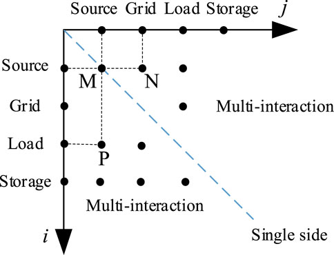
FIGURE 2. Two-dimensional structural model of source–grid–load–storage decision indexes.

From Figures 1, 2, the security impact and economic benefits generated by the energy flow of each part of the complex grid are analyzed. Its investment decision index system contains unilateral indexes of source–grid–load–storage and interactive indexes of grid–source, load–grid, source–load, source–storage, grid–storage, and load–storage. The decision indexes are selected according to the principles of comprehensiveness, comparability, operability, and qualitative with quantitative combination. On the power side, the single-side indexes in Figure 4 are selected to measure the operational characteristics of the complex grid under high penetration of new energy. On the grid side, the single-side indexes in Figure 5 are selected to measure its security. On the load side, the single-side indexes in Figure 6 are selected to measure its participation in the grid regulation process and its impact on the grid. On the electrochemical energy storage side, the single-side indexes in Figure 7 are selected to measure its degree of interaction with the complex grid and its own technical sophistication. In terms of single-side indexes, each side contains four quantitative indexes and one qualitative index. On the interaction side, each side contains four economic efficiency indexes (quantitative indexes), of which the first two indexes are the interaction benefits and the next two indexes are the annual investment benefit ratio and payback period. The adoption of an index system with a completely consistent structure on each side of the source–grid–load–storage can ensure the accuracy of subsequent weighting using the ANP and AHP.

4.1 Calculation of the qualitative index

The unilateral subjectivity index (Q) for each side of the source–grid–load–storage is calculated from the four attributes (S1 to S4) in Figure 3 under different risk states (W₁ to W₃).

FIGURE 3

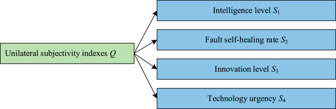
FIGURE 3. Unilateral subjectivity index.

Step 1: Determine the fuzzy level and its corresponding triangular fuzzy number.

The set of hesitant fuzzy linguistic terms is represented by the triangular fuzzy number $\stackrel{\sim }{x}=\left({\stackrel{\sim }{x}}^l,{\stackrel{\sim }{x}}^m,{\stackrel{\sim }{x}}^u\right)$. The fuzzy rank of the triangular fuzzy number (very poor, poor, rather poor, normal, good, and very good) is used to represent the scoring of the experts, and the set of linguistic terms is $\stackrel{\sim }{\mathrm{S}}=\left\{{\mathrm{S}}_0{,\mathrm{S}}_1{,\mathrm{S}}_2{,\mathrm{S}}_3{,\mathrm{S}}_4{,\mathrm{S}}_5{,\mathrm{S}}_6\right\}$. M = {1, 2, …, m}, N = {1, 2, …, n}, and T = {1, 2, …, t}.

X = {X₁, X₂, …, X_m} represents the set of m alternatives, where X_j represents the jth alternative, j∈M. Y = {Y₁, Y₂, …, Y_n} represents the set of n attributes, where Y_i represents the ith attribute, i∈N. w = {w₁, w₂, …, w_n} represents the set of n weights, where w_i represents the weight of attribute Y_i satisfying w_i ≥ 0 and ${\displaystyle \sum }_{i=1}^n{\omega }_i=1$. W = {W₁, W₂, …, W_k} represents the set of natural states, k∈T, in Supplementary Appendix Tables SA1–SA3. The risk-based multi-attribute decision matrix table given by the expert is shown in Supplementary Appendix S1. There are three natural states of W₁, W₂, and W₃ and four attributes of Y₁, Y₂, Y₃, and Y₄.

The optimal value of each attribute for each alternative for different states of nature is determined to be the positive ideal point of the attribute value and is expressed as Eq. 1:

${\stackrel{\sim }{x}}_i^{k+}=\{\begin{array}{l}\left(\underset{1\le j\le m}{\max }\left\{x_{ji}^{kl}\right\},\underset{1\le j\le m}{\max }\left\{x_{ji}^{km}\right\},\underset{1\le j\le m}{\max }\left\{x_{ji}^{ku}\right\}\right),c\in N_b,\\ \left(\underset{1\le j\le m}{\min }\left\{x_{ji}^{kl}\right\},\underset{1\le j\le m}{\min }\left\{x_{ji}^{km}\right\},\underset{1\le j\le m}{\min }\left\{x_{ji}^{ku}\right\}\right),c\in N_c.\end{array}(1)$

According to equation Eq. 1, the positive ideal points of state W₁ can be taken as ${\stackrel{\sim }{x}}_1^{1+}$, ${\stackrel{\sim }{x}}_2^{1+}$, ${\stackrel{\sim }{x}}_3^{1+}$, ${\stackrel{\sim }{x}}_4^{1+}$. The positive ideal points of state W₂ are ${\stackrel{\sim }{x}}_1^{2+}$, ${\stackrel{\sim }{x}}_2^{2+}$, ${\stackrel{\sim }{x}}_3^{2+}$, ${\stackrel{\sim }{x}}_4^{2+}$. The positive ideal points of state W₃ are ${\stackrel{\sim }{x}}_1^{3+}$, ${\stackrel{\sim }{x}}_2^{3+}$, ${\stackrel{\sim }{x}}_3^{3+}$, ${\stackrel{\sim }{x}}_4^{3+}$.

Step 2: Normalization of the matrix.

The decision matrix D can be normalized using the following equation to eliminate the influence of different physical magnitudes on the index values, thus obtaining the normalized decision matrix B. equation.

$B={\left[{\stackrel{\sim }{b}}_{ji}^k\right]}_{m\times n\times t},{\stackrel{\sim }{b}}_{ji}^k=\left({\stackrel{\sim }{b}}_{ji}^{kl},{\stackrel{\sim }{b}}_{ji}^{km},{\stackrel{\sim }{b}}_{ji}^{k\mu }\right)=\{\begin{array}{l}\left({\stackrel{\sim }{x}}_{ji}^{kl}/x_i^{k\mu +},{\stackrel{\sim }{x}}_{ji}^{km}/x_i^{km+},\left({\stackrel{\sim }{x}}_{ji}^{ku}/x_i^{kl+}\right)\wedge 1\right),j\in M,i\in N_b,k\in T,\\ \left({\stackrel{\sim }{x}}_j^{kl+}/x_{ji}^{ku},{\stackrel{\sim }{x}}_i^{km+}/x_i^{km},\left({\stackrel{\sim }{x}}_i^{ku+}/x_{ji}^{kl}\right)\wedge 1\right),j\in M,i\in N_c,k\in T.\end{array}(2)$

Step 3: Regret perception computing.

Regret perception is calculated by the following equation.

$R\left(\Delta \stackrel{\sim }{b}\right)=1-\exp \left(-\delta \Delta \stackrel{\sim }{b}\right),(3)$

where δ (δ > 0) is the regret avoidance coefficient, which represents the difference between the utility values of the two options. The larger the δ is, the greater the degree of regret avoidance of the decision maker. According to Eq. 4, the obtained perceived attribute values for each attribute in the plan are as follows.

$\begin{array}{l}{\stackrel{\sim }{h}}_{ji}^k={\stackrel{\sim }{b}}_{ji}^k+R\left(\Delta \stackrel{\sim }{b}\right)={\stackrel{\sim }{b}}_{ji}^k+1-\exp \left(-\delta \Delta \stackrel{\sim }{b}\right)={\stackrel{\sim }{b}}_{ji}^k+1-\exp \left(-\delta \left({\stackrel{\sim }{b}}_{ji}^k-{\stackrel{\sim }{b}}_i^{k+}\right)\right),\\ {\stackrel{\sim }{b}}_i^{k+}=\left(\underset{1\le j\le m}{\max }\left({\stackrel{\sim }{b}}_{ji}^{ku}\right),\underset{1\le j\le m}{\max }\left({\stackrel{\sim }{b}}_{ji}^{km}\right),\underset{1\le j\le m}{\max }\left({\stackrel{\sim }{b}}_{ji}^{kl}\right)\right).\end{array}(4)$

Then, the regret perception decision matrix is $H={\left[{\stackrel{\sim }{h}}_{\stackrel{\sim }{j}}^k\right]}_{m\times k\times t}$.

Step 4: The group utility value and individual regret value can be solved by Eq. 5.

$\begin{array}{l}{S}_j^k={\displaystyle \sum }_{i=1}^n{\omega }_i\Vert {\stackrel{\sim }{h}}_i^{k+}-{\stackrel{\sim }{h}}_{ji}^k\Vert /\Vert {\stackrel{\sim }{h}}_i^{k+}-{\stackrel{\sim }{h}}_i^{k-}\Vert ,R_j^k=\underset{1\le i\le n}{\max }\left[{\omega }_i\Vert {\stackrel{\sim }{h}}_i^{k+}-{\stackrel{\sim }{h}}_{ji}^k\Vert /\Vert {\stackrel{\sim }{h}}_i^{k+}-{\stackrel{\sim }{h}}_i^{k-}\Vert \right],\\ {\stackrel{\sim }{h}}_i^{k+}=\left(\underset{i\le j\le m}{\max }\left\{h_{ji}^{kl}\right\},\underset{i\le j\le m}{\max }\left\{h_{ji}^{km}\right\},\underset{i\le j\le m}{\max }\left\{h_{ji}^{ku}\right\}\right\},{\stackrel{\sim }{h}}_i^{k-}=(\underset{i\le j\le m}{\min }\left\{h_{ji}^{kl}\right\},\underset{i\le j\le m}{\min }\left\{h_{ji}^{km}\right\},\underset{i\le j\le m}{\min }\left\{h_{ji}^{ku}\right\}].\end{array}(5)$

Step 5: Decision values for subjective indexes are shown as Eq. 6.

$\begin{array}{l}{Q}_j^k=\frac{v\left(S_j^k-S^{k+}\right)}{S^{k-}-S^{k+}}+\frac{\left(1-v\right)\left(R_j^k-R^{k+}\right)}{R^{k-}-R^{k+}},\\ Q_j={\displaystyle \sum }_{k=1}^t{p}^k{Q}_j^k,j\in M,k\in T,\end{array}(6)$

where $S^{k+}=\underset{l\le j\le m}{\min }{S}_j^k$, $S^{k-}=\underset{l\le j\le m}{\max }{S}_j^k$, $R^{k+}=\underset{l\le j\le m}{\min }{R}_j^k$, and $R^{k-}=\underset{I\le j\le m}{\max }{R}_j^k$, and the value of v is 0.5 in this study.

Step 6: Solving the optimal solution.

$\begin{array}{l}\min Q_j\\ \begin{array}{l}\mathrm{s}.\mathrm{t}.p_k^l\le p_k\le p_k^u,k\in T,\\ {\displaystyle \sum }_{k=1}^t{p}_k=1,\end{array}\\ Q_j={\displaystyle \sum }_{k=1}^t{p}^k{Q}_j^k,j\in M,k\in T.\end{array}(7)$

It should be noted that Q_j is the calculated minimal index, which needs to be transformed into a maximal index when performing the calculation of the combined value of indexes. The values of Q_j are shown in Supplementary Appendix Table S4. In the subsequent calculation of the combined value of indexes for the project to be built, Q_j is used to represent the combined value of indexes S₁, S₂, S₃, and S₄. The calculation results are shown in Supplementary Appendix S1.

4.2 Calculation of quantitative indexes on the source side

The wind speed is simulated as follows:

$f_w\left(v\right)=\frac{k}{c}{\left(\frac{v}{c}\right)}^{k-1}\exp \left[-{\left(\frac{v}{c}\right)}^k\right],(8)$

$P_w=\{\begin{array}{ll}0& v⩽v_{\text{ci}},v⩾v_{\text{co}}\\ P_{\mathrm{r}}\ast \frac{v^3-v_{\text{ci}}^3}{v_{\mathrm{r}}^3-v_{\text{ci}}^3}& v_{\text{ci}}<v<v_{\mathrm{r}}\\ P_{\mathrm{r}}& v_{\mathrm{r}}<v<v_{\text{co}}\end{array}.(9)$

In Eq. 8, c and k are the scale and shape parameters, respectively, and c reflects the average wind speed of the wind power plant. c is taken as 22.64 and v as 24.1. The wind power output is calculated as follows. In Eq. 9, v_ci is the cut-in wind speed, v_r is the rated wind speed, and v_co is the cut-out wind speed. The calculation method of photovoltaic output is the same as that of wind power and will not be repeated here.

The source-side investment decision indexes are shown in Figure 4.

FIGURE 4

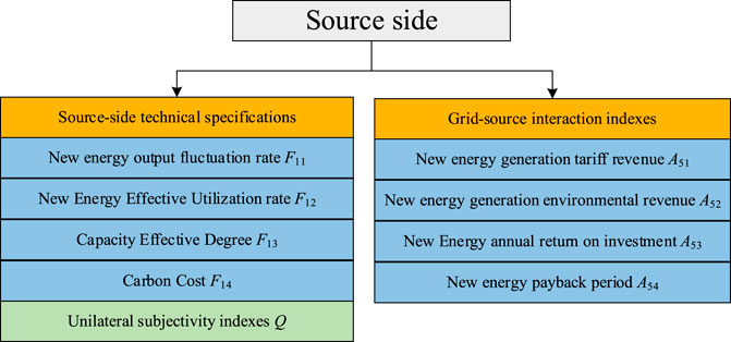
FIGURE 4. Source-side investment decision indexes.

The new energy output fluctuation rate (Liou and Wang Maojiun, 1992) is calculated as Eq. 10.

$F_{11}=\frac{P_{\max }^{NE}-P_{\min .}^{NE}}{P_{\max }^{NE}}(10)$

PNE max is the maximum power generated by new energy in a typical day, MW; PNE min is the minimum power generated by new energy in that day, MW.

The new energy effective utilization rate (Zhao et al., 2015) is calculated as Eq. 11.

$F_{12}=\frac{E_{\text{NG}}^{NE\ast }}{P_{NG}^{NE}\mathrm{T}}.(11)$

ENE* NG is the actual annual output of new energy, MW·h; PNE NG is the installed capacity of new energy, MW; and T is 8760 hours (total number of hours in a year).

The capacity effective degree is calculated as Eq. 12.

$F_{13}=\frac{E_{\text{NG}}^{NE\ast }}{E_{all}^{*}}.(12)$

E* all is the actual annual generation capacity of all units, MW·h.

Carbon cost is calculated as Eq. 13.

$F_{14}=k_{{\text{CO}}_2}{E}_{\text{NG}}^{NE*}{\lambda }_{{\text{CO}}_2}*0.1.(13)$

In the aforementioned Eq. 13, k_CO2 is the carbon emission factor, and the typical value of the carbon emission factor of the southern power grid (Zhang et al., 2018) is 0.5721 kg/(kW·h), λCO₂ is the unit carbon emission trading price of 0.0585 yuan/kg, and the unit of F_14,power is 10000 yuan.

New energy generation tariff revenue is calculated as Eq. 14.

$A_{51}=E_{\text{NG}}^{NE*}*M_{Newenergy}*0.1.(14)$

M_Newenergy is the new energy generation tariff, yuan/(kW·h), and the unit of A_51,G-p is million yuan.

New energy generation environmental revenue is calculated as Eq. 15.

$A_{52}=E_{\text{NG}}^{NE*}*k_{{\text{CO}}_2}*M_{Carbon}*0.1.(15)$

M_Carbon is the unit price of the environmental revenue of new energy generation, yuan/kg, and the unit of A_52,G-p is 10000 yuan.

New energy annual return on investment is calculated as Eq. 16.

$\{\begin{array}{l}Annua{l}_{Powercost}=\left(\left(1+x_{wp}\%\right)c_{wp}{E}_{wp}\right)\frac{{\left(1+r\right)}^{T_{\text{Lifespanp}}}r}{{\left(1+r\right)}^{T_{\text{Lifespanp}}}-1}Photovoltaic,\\ Annua{l}_{Powercost}=\left(\left(1+x_{ww}\%\right)c_{ww}{E}_{ww}\right)\frac{{\left(1+r\right)}^{T_{\text{Lifespanw}}}r}{{\left(1+r\right)}^{T_{\text{Lifespanw}}}-1}Wind,\\ A_{53}=\frac{A_{51}+A_{52}}{Annua{l}_{Powercost}}.\end{array}(16)$

c_wp and c_ww are the unit power price of photovoltaic and wind power, million/MW; E_wp and E_ww are the rated power of photovoltaic and wind power, MW, respectively. T_lifespanp and T_lifespanw are the full life cycle of photovoltaic and wind power, years; r is the social average annual return on investment, which is taken as 8% in this study. x_wp% and x_ww% are the ratio of the operating cost and initial investment of photovoltaic and wind power, respectively. The unit of Annual_powercost is 10000 yuan.

The new energy payback period is calculated as Eq. 17.

$A_{54}=\{\begin{array}{l}\frac{Annua{l}_{Powercost}*T_{\text{Lifespanp}}}{A_{51}+A_{52}}Photovoltaic,\\ \frac{Annua{l}_{Powercost}*T_{\text{Lifespanw}}}{A_{51}+A_{52}}Wind.\end{array}(17)$

4.3 Calculation of quantitative indexes on the grid side

The grid-side investment decision indexes are shown in Figure 5.

FIGURE 5

FIGURE 5. Grid-side investment decision indexes.

Network coordination is calculated as Eq. 18.

$F_{21}=\frac{P_{\max }^{NE}-P_{\min }^{NE}}{P_{\max }^{NE}}.(18)$

N_L is the total number of power grid lines, L_k is the load rate of the ith line, and $\stackrel{-}{L}$ is the average of the load rates of N_L lines.

The N-1 pass rate is calculated as Eq. 19, and N_p is the number of lines that passes the N-1 security check.

$F_{22}=\frac{N_{\mathrm{p}}}{N_{\mathrm{L}}}.(19)$

Grid loss is calculated as Eq. 20.

$F_{23}={\displaystyle \sum }_{\left(ij\right)\in {\Omega }_l}\left[g_{ij}\left(V_i^2+V_j^2-2V_i{V}_j\cos {\theta }_{ij}\right)\right]*{10}^{-6}.(20)$

Ω_l is the set of all branches in the grid. V_i and V_j are the voltage amplitudes of nodes i and j in the grid, respectively. g_ij and ϴ_ij are the conductance and phase angle differences of nodes i and j in the grid, respectively. The unit of F_23,grid is MW.

The grid heavy load rate is calculated as Eq. 21.

$F_{24}=\frac{N_{\text{HL}}}{N_{\mathrm{L}}}.(21)$

N_HF is the number of heavy load lines. In this study, the annual maximum load rate exceeds 70% and lasts for more than 1 hour as a heavy load line.

Revenue from additional electricity sales is calculated as Eq. 22.

$A_{61}=E_{IE}^{Loss*}*M_{\text{Grid}}*0.1.(22)$

ELoss* IE is the annual incremental electricity sales, MW·h. M_Grid is the electricity sale price, yuan/(kW·h). The unit of A_61,L-g is 10,000 yuan.

Political subsidy from reduced grid loss is calculated as Eq. 23.

$A_{62}=E_{IE}^{Loss*}*M_{\text{Grid}}*0.1.(23)$

M_reward is the unit price of the reward, yuan/(MW·h). The unit of A_62,L-g is 10000 yuan.

New line annual return on investment is calculated as Eq. 24:

$\{\begin{array}{l}Annua{l}_{gridcost}=\left(\left(1+x_g\%\right)c_g{L}_g\right)\frac{{\left(1+r\right)}^{T_{\text{Lifespang}}}r}{{\left(1+r\right)}^{T_{\text{Lifespang}}}-1},\\ A_{63}=\frac{A_{61}+A_{62}}{Annua{l}_{gridcost}}.\end{array}(24)$

c_g is the cost per kilometer of the transmission line, 10000 yuan/km. L_g is the length of the transmission line, km. T_lifespang is the full life cycle of the transmission line, years. x_g% is the ratio of the operating cost of the transmission line to the initial investment. The unit of Annual_gridrcost is 10000 yuan.

The new line payback period is calculated as Eq. 25.

$A_{64}=\frac{Annua{l}_{gridrcost}*T_{\text{Lifespang}}}{A_{61}+A_{62}}.(25)$

4.4 Calculation of quantitative indexes on the load side

The load-side investment decision indexes are shown in Figure 6.

FIGURE 6

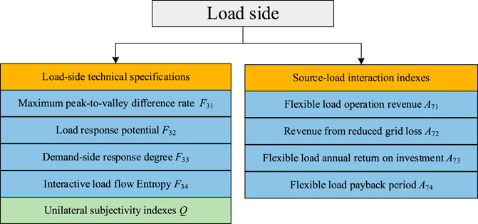
FIGURE 6. Grid-side investment decision indexes.

The maximum peak-to-valley difference rate is calculated as Eq. 26, and PLoad t is the power of the flexible load at moment t in day D, MW. $\underset{t\in D}{\max }\left(P_t^{Load}\right)$ and $\underset{t\in D}{\min }\left(P_t^{Load}\right)$ are the maximum and minimum values of the flexible load on day D, respectively.

$F_{31}=\frac{\left(\underset{t\in D}{\max }\left(P_t^{Load}\right)-\underset{t\in D}{\min }\left(P_t^{Load}\right)\right)}{\underset{t\in D}{\max }\left(P_t^{Load}\right)}.(26)$

Load response potential is calculated as Eq. 27.

$F_{32}==\{\begin{array}{l}\frac{P_{i,\max }\left(t\right)-P_{i,0}\left(t\right)}{P_{i,0}\left(t\right)},Increasedpowerafter\mathrm{int}eraction,\\ \frac{P_{i,\min }\left(t\right)-P_{i,0}\left(t\right)}{P_{i,0}\left(t\right)},Decreasedpowerafter\mathrm{int}eraction.\end{array}(27)$

P_i,max(t), P_i,min(t), and P_i,0(t) are the maximum power, minimum power, and rated power that can be reached after the flexible load participates in the demand-side response at time t, respectively, all in MW.

The demand-side response degree is calculated as Eq. 28, and P_i(t) is the actual interactive power of the flexible load, MW.

$F_{33}=\frac{P_i\left(t\right)-P_{i,0}\left(t\right)}{P_{i,0}\left(t\right)F_{32,load}\left(t\right)}.(28)$

Interactive load flow entropy is calculated as Eq. 29.

$F_{34}=-\ln 10{\displaystyle \sum }_j^{n-1}\frac{l_j}{N_L}\ln N_L.(29)$

Given a constant sequence R = {R₁,R₂,R₃,…,R_n}, l_j is the number of lines whose load rate r_j satisfies r_j∈(R_j,R_j+1].

In this study, the internet data center load is used as an example of a revenue stream in the form of rack rental, IT electricity tax credit revenue, settlement revenue, and bandwidth revenue. Flexible load operation revenue is calculated as Eq. 30.

$A_{71}=P_{i,0}\left(t\right)*M_{\text{IDC}}*100.(30)$

M_IDC is the unit revenue of the internet data center, yuan/W·years. The unit of A_72,P-l is 10000 Yuan.

Revenue from reduced grid loss is calculated as Eq. 31.

$A_{72}=\left(E_{BeforeLoad}^{Loss*}-E_{AfterLoad}^{Loss*}\right)*M_{\text{Grid}}.(31)$

ELoss* BeforeLoad and ELoss* AfterLoad are the total annual loss of the grid before and after the new flexible load, MW. The unit of A_71,P-l is 10000 yuan.

Flexible load annual return on investment is calculated as Eq. 32.

$\{\begin{array}{l}Annua{l}_{Loadcost}=\left(\left(1+x_l\%\right)c_l{P}_l\right)\frac{{\left(1+r\right)}^{T_{\text{Lifespanl}}}r}{{\left(1+r\right)}^{T_{\text{Lifespanl}}}-1},\\ A_{73}=\frac{A_{71}+A_{72}}{Annua{l}_{Loadcost}}.\end{array}(32)$

c_l is the price per unit power of the flexible load, million/(MW·h). P_l is the rated power of the flexible load, MW·h. T_lifespanl is the full life cycle of the flexible load, years. x_l% is the ratio of the operating cost of the flexible load to the initial investment, and the unit of Annual_loadcost is 10000 yuan.

The flexible load payback period is calculated as Eq. 33.

$A_{74}=\frac{Annua{l}_{Powercost}*T_{\text{Lifespanw}}}{A_{71}+A_{72}}(33)$

4.5 Calculation of quantitative indexes on the storage side

The storage-side investment decision indexes are shown in Figure 7. The electrochemical energy storage whole life cycle cost is calculated as Eq. 34.

$F_{41}=\left(\left(1+x_s\%\right)c_e{E}_{storage}+\left(1+y_s\%\right)c_p{P}_{storage}\right)\frac{{\left(1+r\right)}^{T_{\text{Lifespan}}}r}{{\left(1+r\right)}^{T_{\text{Lifespan}}}-1}.(34)$

c_e and c_p are the price per unit capacity and the price per unit power of electrochemical energy storage, respectively, 10000 yuan/(MW·h). E_storage and P_storage are the rated capacity (MW·h) and rated power (MW) of the electrochemical energy storage power plant, respectively, and T_lifespan is the whole life cycle of the electrochemical energy storage power plant. x_s% and y_s% are the ratio of the operating cost of electrochemical energy storage capacity and power to initial investment. F_41,storage is in million yuan.

FIGURE 7

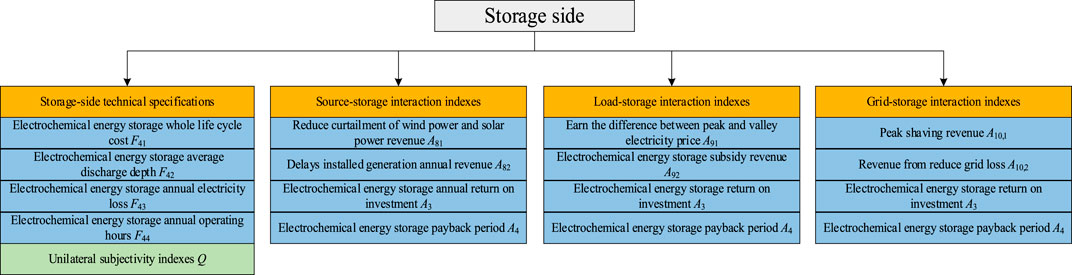
FIGURE 7. Storage-side investment decision indexes.

The electrochemical energy storage average discharge depth is calculated as Eq. 35.

$F_{42}=\frac{1}{k}{\displaystyle \sum }_{i=1}^{k}E{D}_i.(35)$

ED_i is the electricity released during the ith discharge of the electrochemical energy storage system, MW. k is the number of discharges of the electrochemical energy storage device during the year.

Electrochemical energy storage annual electricity loss is calculated as Eq. 36.

$F_{43}={\displaystyle \sum }_{t=1}^{\mathrm{T}}\left(u_t^{ESS}{P}_t^{ESS,c}-v_t^{ESS}{P}_t^{ESS,d}\right).(36)$

PESS,c t and PESS,d t are the charging and discharging power of the electrochemical energy storage at hour t, MW, respectively. uESS t and vESS t are the charging and discharging characteristic variables of the electrochemical energy storage, respectively, and cannot be 1 at the same time. When uESS t = 1 and vESS t = 0, the electrochemical energy storage plant is in the charging state. When uESS t = 0 and vESS t = 1, the electrochemical energy storage plant is discharging. When uESS t = 1 and vESS t = 0, the storage plant is in the static state. F_43,storage is in MW.

The electrochemical energy storage annual operating hours are calculated as Eq. 37.

$F_{44}={\displaystyle \sum }_{t=1}^{\mathrm{T}}\left(u_t^{ESS}+v_t^{ESS}\right).(37)$

Reduced curtailment of wind power and solar power revenue is calculated as Eq. 38.

$A_{81}=\left(E_{\text{AW}}+E_{\text{AP}}\right)*M_{P-s}.(38)$

E_AW and E_AP are the annual abandoned wind power and abandoned photovoltaic power reduced by the electrochemical energy storage, respectively, MW·h. M_P-s is the reward coefficient, 10000 yuan/(MW·h). The unit of A_81, is 10000 yuan.

Delayed installed generation annual revenue is calculated as Eq. 39, and e_r denotes the price per unit of power backup capacity, million/(MW·h). The unit of A_82,P-s is million yuan.

$A_{82}=e_r{\displaystyle \sum }_{t=1}^{\mathrm{T}}{v}_t^{ESS}{P}_t^{ESS,d}.(39)$

The difference earned between peak and valley electricity prices is calculated as Eq. 40.

$A_{91}=\Delta Q\left(p_f-p_g\right)*0.1.(40)$

ΔQ is the total amount of electricity charged through the electrochemical energy storage system throughout the year, MW·h. P_f and P_g are the peak and valley tariffs implemented in the region, respectively, yuan/(kW·h). A_91,L-s are in million yuan.

The electrochemical energy storage subsidy revenue (Han et al., 2014) is calculated as Eq. 41.

$A_{92}=\Delta p_f{m}_f*0.1.(41)$

ΔP_f is the annual peak load reduction after grid access to electrochemical energy storage, MW·h. m_f is the reward received per unit peak load reduction, yuan/(kW·h). The unit of A_92,L-s is 10000 yuan.

The peak-shaving revenue is calculated as Eq. 42.

$A_{\mathrm{10,1}}=e_m{P}_{RC}*0.1.(42)$

e_m is the unit peaking revenue of electrochemical energy storage, yuan/(kW·h). P_RC is the annual peaking electricity of electrochemical energy storage, MW·h. The unit of A_10,1,G-s is 10000 yuan.

Revenue from reduced grid loss is calculated as Eq. 43.

$A_{\mathrm{10,2}}={{\displaystyle \sum }_{i=1}^{N^T}\Delta Q}_{loss}*M_{\text{Grid}}*0.1.(43)$

ΔQ_loss represents the amount of change in grid loss before and after new electrochemical energy storage, MW. The unit of A_10,2,G-s is 10000 yuan.

Let the electrochemical energy storage and source–grid–load interaction revenue be A_1,s and A_2,s.

The electrochemical energy storage return on investment is calculated as Eq. 44.

$A_3=\frac{A_{1,s}+A_{2,s}}{F_{41}}.(44)$

The electrochemical energy storage payback period is calculated as Eq. 45.

$A_4=\frac{F_{41,storage}*T_{\text{Lifespan}}}{A_{1,s}+A_{2,s}}.(45)$

5 Determination of index weights

5.1 Entropy weight method

The basic principle of the entropy weight method is to assign different weights to the data according to the magnitude of data variation, which is expressed by information entropy.

$H\left(x\right)=-{\displaystyle \sum }_{i=1}^n\left[p\left(x_i\right)\ln \left(p\left(x_i\right)\right)\right].(46)$

x is a situation in which event X happens. Then, the probability of this situation happening is p(x) and n is the number of items.

Applying EWM to the calculations in this study, the index matrix first needs to be standardized matrix Z. The following Eq. 47 is the standardization equation.

$\stackrel{\sim }{z_{ij}}=\frac{x_{ij}-\min \left\{x_{1j},x_{2j},\dots x_{nj}\right\}}{\max \left\{x_{1j},x_{2j},\dots x_{nj}\right\}-\min \left\{x_{1j},x_{2j},\dots x_{nj}\right\}}.(47)$

Then, the weight of the ith item under the jth index is calculated and considered the probability in the relative entropy calculation: ${\mathrm{p}}_{\mathrm{i}\mathrm{j}}={\mathrm{z}}_{\mathrm{i}\mathrm{j}}/{\displaystyle \sum }_{\mathrm{i}=1}^{\mathrm{n}}{\mathrm{z}}_{\mathrm{i}\mathrm{j}}$, which is then normalized by the information entropy calculation equation.

$e_j=-\frac{1}{\ln n}{\displaystyle \sum }_{i=1}^n{p}_{ij}\ln \left(p_{ij}\right).(48)$

Finally, the entropy weight of the indexes is calculated.

$W_j=\left(1-e_j\right)/{\displaystyle \sum }_{j=1}^m\left(1-e_j\right).(49)$

In Eq. 49, m is the number of indexes.

5.2 Analytic network process

The ANP is an extension of the AHP which is mainly aimed at situations where the structure of the decision problem is dependent and feedback-oriented. The structure of the ANP is in the form of a network cycle, where one level of the system can be both dominant and indirectly dominated by other levels, which can be represented by a network with nodes, as shown in Figure 8 below.

FIGURE 8

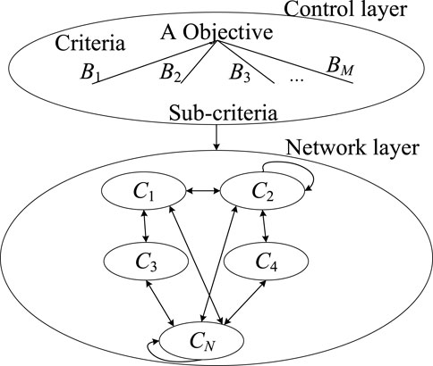
FIGURE 8. ANP structure diagram.

As can be seen from the aforementioned figure, the ANP divides the system elements into the control layer and network layer. The control layer consists of a decision objective A and a decision criterion (B₁, B₂, …, B_M). The network layer consists of all the element groups (C₁, C₂, …, C_N) that are subject to the decisions of the control layer. The elements in the element group C_i (i = 1, …, N) are e_i1, e_i2, …, e_ini.

By Figure 9, the calculation flow of ANP is as follows:

FIGURE 9

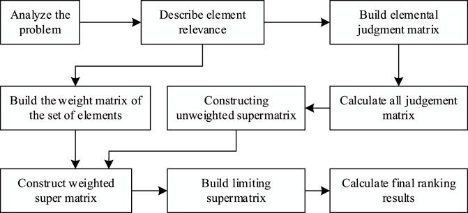
FIGURE 9. ANP calculation workflows.

Step 1: Describe the element relevance, build and calculate the element judgment matrix, and construct the unweighted supermatrix.

With the control layer B_k as the criterion and the element e_jt(e_j1, e_j2, …, e_jnj) in C_j(j = 1, …, N) as the sub-criterion. The elements in the element set C_i build the judgment matrix according to their degree of influence on the elements in C_j.

In Eq. 50, the column vector of W_ij is the column vector of the degree of influence of the elements in the element set C_i on its own elements, whose value is shown in Supplementary Appendix Tables SB5–SB16.

$W_{ij}=[\begin{array}{l}{w}_{i1}^{\left(j1\right)}{w}_{i1}^{\left(j2\right)}\cdots \\ w_{i2}^{\left(\mathrm{j}1\right)}{w}_{i2}^{\left(j2\right)}\cdots \\ ⋮\\ w_{i{n}_i}^{\left(j1\right)}{w}_{i{n}_i}^{\left(j2\right)}\cdots \end{array}\begin{array}{l}{w}_{i1}^{\left(j{n}_j\right)}\\ w_{i2}^{\left(j{n}_j\right)}\\ \\ w_{i{n}_i}^{\left(j{n}_j\right)}\end{array}].(50)$

Then, the unweighted supermatrix W is constituted by the degree of influence of all elements in the element set C_i(i = 1,..., N) on all elements in the element set C_j(j = 1,..., N) under the criterion B_k as Eq. 51.

$\begin{array}{l}1\cdots n_{1}1\cdots n_2\cdots 1\cdots n_N\\ W=\begin{array}{l}1\cdots n_1\\ 1\cdots n_2\\ ⋮\\ 1\cdots n_N\end{array}[\begin{array}{l}{\mathit{W}}_{11}{\mathit{W}}_{12}\cdots \\ {\mathit{W}}_{21}{\mathit{W}}_{22}\cdots \\ ⋮\\ {\mathit{W}}_{N1}{\mathit{W}}_{N2}\cdots \end{array}\begin{array}{l}{\mathit{W}}_{1N}\\ {\mathit{W}}_{2N}\\ \\ {\mathit{W}}_{NN}\end{array}]\end{array}.(51)$

Step 2: Build the weighting matrix of the set of elements.

Taking the control layer B_k as the criterion, a weighting matrix is constructed for the degree of influence of the element set C_i on C_j.

Then, the weighting matrix D is Eq. 52, whose value is shown in Supplementary Appendix Tables SB3–SB4.

$D=[\begin{array}{l}{d}_{11}\cdots \\ d_{21}\cdots \\ ⋮\\ d_{N1}\cdots \end{array}\begin{array}{l}{d}_{1N}\\ d_{2N}\\ \\ d_{NN}\end{array}],(52)$

Step 3: Using the weighting matrix D to assign weights to the unweighted supermatrix W to obtain the weighted supermatrix as Eq. 53. The value of W is shown in Supplementary Appendix Tables SB17.

$\stackrel{—}{W_{ij}}=d_{ij}{W}_{ij}.(53)$

Step 4: Build the limiting matrix and obtain the weights of each element.

The elements in the weighted supermatrix $\overline{W}$ are still W_ij, which reflects the first-step dominance of element i over element j, recorded as a ${\overline{W}}^{\left(1\right)}$. The value of $\overline{W}$ is shown in Supplementary Appendix Tables SB18. The second-step dominance of element i over element j is ${\displaystyle \sum }_{m=1}^N{W}_{im}^{\left(1\right)}{W}_{mj}^{\left(1\right)}$, recorded as ${\overline{W}}^{\left(2\right)}$. The limiting dominance is the cumulative effect of influence so that the tth-step dominance of element i over element j is as Eq. 54.

${\overline{W}}_{ij}^{\left(t\right)}={\displaystyle \sum }_{m=1}^N{\overline{W}}_{im}^{\left(t-1\right)}{\overline{W}}_{mj}^{\left(t-1\right)}.(54)$

The limit exists when ${\overline{W}}^{\left(t\right)}$ is at $t\to \infty$, i.e.,

${\overline{W}}^{\left(\infty \right)}=\underset{t\to \infty }{\lim }{\overline{W}}^{\left(t\right)}.(55)$

Then, the jth column of ${\overline{W}}^{\left(\infty \right)}$ is the weight of each element under B_k. The value of ${\overline{W}}^{\left(\infty \right)}$ is shown in Supplementary Appendix Tables SB19.

5.3 Combined weighting method

The combined weighting method is used to assign weights to complex grid investment indexes so that decision makers can take advantage of their own experience in the decision-making process and avoid the subjective arbitrariness of assigning weights. This study adopts the game theory approach to obtain the combination weights and uses W to represent the weight vector of combination weights, W_a to represent the weight vector derived from the ANP, and W_e to represent the weight vector derived from EWM. According to the Nash equilibrium principle, the optimal value of the combination weight W should be the equilibrium state between the two sides of the game, when the sum of the deviations of W and W_a and W_e is the smallest.

The optimal linear combination coefficients α* and β* are found with the objective function of minimizing the sum of the deviations of W and W_a and W and W_e (Liu et al., 2021). Then, the objective function and constraints for the calculation of W are as Eq. 56.

$\begin{array}{l}\min \left(\Vert W-W_a{\Vert }_2+\Vert W-W_e{\Vert }_2\right)\\ =\min \left(\Vert \alpha W_a+\beta W_e-W_a{\Vert }_2+\Vert \alpha W_a+\beta W_e-W_e{\Vert }_2\right),\\ s.t.\alpha +\beta =1,\alpha ,\beta \ge 0.\end{array}(56)$

According to the principle of differentiation, the conditions for the derivative of Eq. 55 to obtain the minimum value are as expressed as Eq. 57.

$\{\begin{array}{l}\alpha W_a{W}_a^T+\beta W_a{W}_e^T=W_a{W}_a^T,\\ \alpha W_e{W}_a^T+\beta W_e{W}_e^T=W_e{W}_e^T.\end{array}(57)$

The values of α and β are then normalized to obtain α* and β*.

${\alpha }^{*}=\frac{\left|\alpha \right|}{\left|\alpha \right|+\left|\beta \right|},{\beta }^{*}=\frac{\left|\beta \right|}{\left|\alpha \right|+\left|\beta \right|}.(58)$

Then, the optimal combination weights are given as Eq. 59.

$W={\alpha }^{\ast }\ast W_a+{\beta }^{\ast }\ast W_e.(59)$

Because both EWM and ANP have their limitations, this study uses EWM and ANP to form a combined weighting method which is used to assign weights to the indexes.

5.4 Investment decision method calculation process

First, we determine the project library to be built and then calculate the investment decision indexes of each side of source–grid–load–storage. After index normalization, we form the investment decision index matrix. The EWM is used to assign objective weights to each index first, and then ANP is used to assign subjective weights to each side index. Finally, the combined value of the indexes is calculated using the distance vector combining algorithm, and the indexes are evaluated according to the size of the combined value of the indexes. The calculation flow chart is shown in the following figure.

6 Simulation and analysis

We consider the example of a power grid in a region of southwest China where there are 16 projects to be built on the source–grid–load–storage side. There are 49 buses and 64 branches in the area, of which there are 4220-kV buses, 13 110-kV buses, and 23 35-kV buses. Among them, there are seven generators with a total generation capacity of 477 MW and a total load of 470 MW. The power-side projects are numbered as power 1, power 2, power 3, and power 4, as shown in Table 1. The grid-side projects are numbered as grid 1, grid 2, grid 3, and grid 4, as shown in Table 2. The load-side projects are numbered as load 1, load 2, load 3, and load 4, as shown in Table 3. The storage projects are numbered as storage 1, storage 2, storage 3, and storage 4, as shown in Table 4. The loan interest rate is 0.08, and the wholesale electricity price is 0.4263 yuan/(kW·h).

TABLE 1

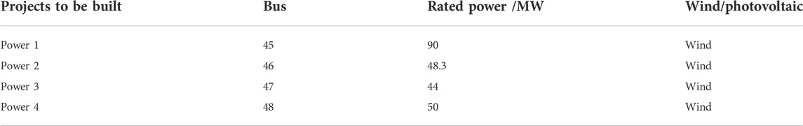
TABLE 1. Basic data of projects to be built on the power side.

TABLE 2

TABLE 2. Basic data of projects to be built on the grid side.

TABLE 3

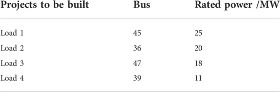
TABLE 3. Basic data of projects to be built on the load side.

TABLE 4

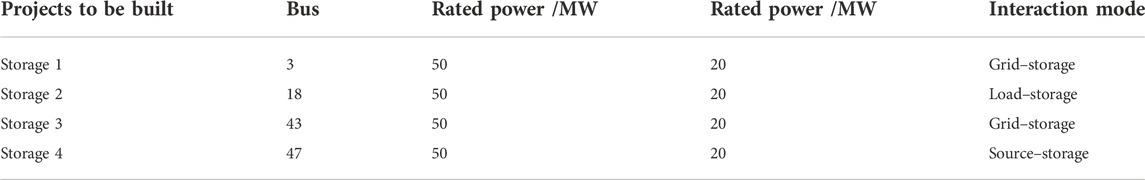
TABLE 4. Basic data of projects to be built on the storage side.

6.1 Calculation of indexes

According to the index calculation method in Section 3, the unilateral indexes and interactive indexes of each side of the source–grid–load–storage are calculated. The unilateral indexes are normalized, and the interactive indexes are not normalized in order to visualize the economic benefits generated by the interaction of each project. F₁∼F₅ are the unilateral indexes of each side, A₁∼A₄ are the interactive indexes of each side, and the values of each index are shown in Table 5.

TABLE 5

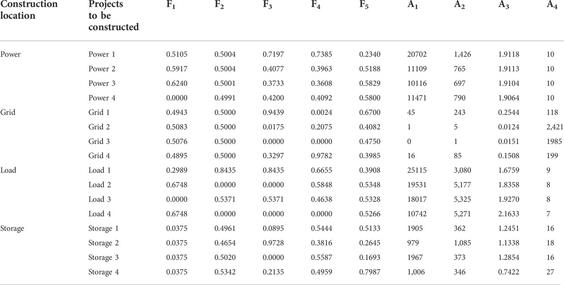
TABLE 5. Per value of indexes.

6.2 Determine the weights

Based on the calculated indexes, the weights are calculated by using the ANP, EWM, and combined weighting method, and the results are shown in Table 6. As can be observed from Figure 10, the weighting curve derived from the combined weighting method lies between the EWM and ANP. Since the degree of variation in the values of indexes F1∼F4 of the projects to be built on the power side is higher, the EWM assigns them larger weights. The decision makers pay more attention to indexes A1∼A4, so the weights assigned to indexes F1∼F4 under the ANP are smaller. Similarly, in indexes A1∼A4, the EWM assigns smaller weights due to the small degree of variation in the values of the indexes of the projects to be built, but the decision makers pay more attention to the interaction of indexes A1∼A4, so the ANP assigns larger weights to them. We can observe from Figure 10 that index F₁ and index F₅ are too small on the power side, index A₁ is too large on the grid side, and index F₅ is too small on the load side and storage side. These too large or too small index weights are not conducive to a comprehensive evaluation of the overall benefits of each project to be built.

TABLE 6

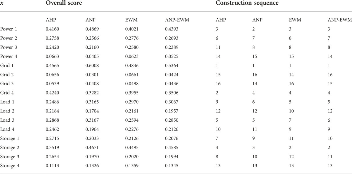
TABLE 6. Integrated investment decision results for different weighting methods.

FIGURE 10

FIGURE 10. The weights calculated by different weighting methods in the complex grid.

The combined weighting method can rationalize and coordinate EWM and ANP, reduce the subjective arbitrariness of the ANP and the objective absoluteness of the EWM, and make the assignment results more in line with reality. The weights calculated by the combined weighting method of the grid side, load side, and storage side are also shown in Figure 10. The weights calculated by the AHP are shown in Supplementary Appendix Tables SC1–SC3.

6.3 Results of investment decisions with different weighting methods

First, comparing the decision results of the ANP and AHP in Table 6, we can see that the first, fifth, twelfth, and thirteenth projects to be built in ANP and AHP are the same, and the second project to be built in ANP is Power 1, while Power 1 is the third project to be built in AHP. The above situation occurs because both ANP and AHP are subjective weighting methods that reflect the subjective preferences of decision makers, but because ANP considers the interaction between indexes, and the size of Power 1’s indexes exactly matches the size of ANP’s weights.

Then comparing the decision results of ANP and EWM, we can see that the first construction project of ANP and EWM is both Grid 1, the second construction project of EWM is Storage 2, While Power 1 is the second project to be built in ANP. Because F3 and A1 indexes contain more information, so they have more weight, while these indexes of Storage 2 are larger. Although the ANP considers the interaction and feedback between the indexes, it cannot reflect the difference in information among indexes. From Table 5, we can clearly see that Power 1 has no significant economic advantage over Storage 2, but Storage 2 has the largest index, F3, of all the indexes, and F3 has a large amount of information.

Further comparing the decision results of the combined weighting method and ANP, we can see that the first construction project of the combined weighting method and ANP is both Grid 1. The second construction project of ANP is Power 1, While the second construction project in combined weighting method is Storage 2. Therefore, the combined weighting method considers the risk preferences of decision makers and takes into account the amount of information contained in the indexes, and the decision results are more reasonable.

Finally, comparing the decision results of the combined weighting method and EWM, we can see that the construction order of their first, second, third, fourth, fifth projects to be built are the same, but the sixth project of the combined weighting method is Load 3, and the sixth project of EWM is Power 2. We can see from Table 5 that the technical indexes of Load 3 are slightly worse than that of Power 2, but its economic indexes are much better. The disadvantage of EWM is that it focuses too much on the information quantity of indexes and lacks the consideration of decision makers’ preferences.

The combined weighting method has the same construction sequence as the ANP and EWM for many projects to be constructed, and it solves the shortcomings of the ANP which only considers the investor’s index preference and the EWM which only focuses on the amount of index information. It achieves the balance of subjective and objective weighting methods, and its decision results are more scientific and reasonable.

7 Analysis and discussion

7.1 Result analysis

As shown in Figures 4–7, this study proposes a complex grid investment decision index system that includes source–grid–load–storage. The indexes of each side of the index system are both unilateral and interactive, and through the interaction of the interactive indexes, source–grid–load–storage forms an organic whole, which can comprehensively evaluate the impact of new projects on the complex grid as an entire, as shown in Figure 1. For example, indexes A₅ and A₆ can both interact with the grid side, where A₅ is the main economic benefit index and A₆ is the environmental and social benefit.

As observed in Figure 10, the weight of the economic indexes (6–9) is generally larger than the weight of the technical indexes (1–5), except for the electrochemical energy storage side, because the ANP takes into account the psychology of decision makers who emphasize economic efficiency by playing against the weights decided by the EWM, thus increasing the weighting of economic indexes in the combined weighting method. Based on our index system and the weighting of each index, it is important to fully consider the economic and social benefits of the project to be built when making complex grid investment decisions.

As can be seen from Table 5, none of the projects to be built is in the lead for all indexes. Grid 2 and Grid 3 have inferior technical and economic indexes, so they are ranked low among all the projects to be built. The index A₃ in Load 4 is larger than Load 1, but because its A₁ significantly smaller, it can only be ranked behind Load 1. It is clear that when comparing projects on different sides of a complex grid with each other, the value of all the indexes for the project with priority construction must be comparatively large. There is also a special case to be made, as we can see in Figure 10, where index A₁ has a decisive advantage on the grid side and projects with a large index A₁ are built first when there is little difference in the other indexes. For example, there are many indexes that Grid 1 does not dominate, but its F₃ and A₁ are the largest of all indexes, so it is the first to be built.

7.2 Determinant analysis

This study presents a complex grid investment decision method, whose main contribution is in the establishment of an index system and study of the weighting method. The first decisive factor is to establish a framework for a source–grid–load–storage interaction index system. This framework must consider the grid–source interaction, the load–grid interaction, the source–load interaction, the source–storage interaction, the load–storage interaction, the grid–storage interaction, and the single-side technical indexes on the source side, the grid side, the load side, and the electrochemical energy storage side. In order to account for the subjective preferences of decision makers, the index system must include the subjective index. We think that the indexes in the index system can be replaced with other indexes as long as they can meet its framework. The provision is that each side of the source–grid–load–side should have single-side indexes and interaction indexes and that the total number of indexes should not exceed nine in order to meet the requirements of the AHP and other weighting methods for consistency. Of the unilateral indexes, the first four are all technical and the last one is all subjective. Of the interactive indexes, the first is the primary benefit, the second is the secondary benefit, and the third and fourth are the return on investment and payback period, respectively. The second decisive factor is the combined weighting method in this study, where one can choose a subjective and an objective weighting method, and the effect of considering the subjective–objective balance can be achieved. However, in order to take full account of the interactions between the various sides of the complex grid, the subjective weighting method is best used with the ANP. It should be noted that when the indexes in the index system change, the interactions and feedback relationships between the indexes will also change, so the supermatrix of the ANP needs to be recalculated.

7.3 Electrochemical energy storage evaluation and future outlook

Electrochemical energy storage has a supporting role in the complex grid, which is shown in Figure 1, so this requires a analysis of its capacity and effectiveness. We observe Table 6, we can find that the construction order of storage1 is before Grid 2, Grid 3, which is because the integrated benefit of grid–storage interaction is larger than the integrated benefit of load–grid interaction. The construction sequence of storage 2 is before load 1, load 2, load 3, and load 4, which proves that the integrated benefit of load–storage interaction is above that of source–load. The construction order of storage 4 is before that of power 4, which proves that the comprehensive benefits of source–storage interaction are above that of grid–source. We can see from the aforementioned analysis that electrochemical energy storage can indeed partially replace the power source, grid, and flexible load to play a corresponding role in the complex grid. Among them, the source–storage interaction mainly plays the role of reducing wind and light abandonment, while the grid–storage interaction mainly plays the role of peak shaving, and its benefit is not as good as the load–storage interaction which earns the peak-to-valley price difference.

The method proposed in this study does not fully take into account the losses and depreciation on each side of the source–grid–load–storage, which can be taken into account in subsequent studies. In addition, this study only considers the impact of two–two interactions in a complex grid, and the interaction of three sides and four sides can be considered in future studies.

8 Conclusion

In this study, a complex grid investment decision index system under the integrated source–grid–load–storage environment was constructed, which includes unilateral indexes of each side of source–grid–load–storage and interactive indexes between source–grid–load–storage. The unilateral indexes include technical benefits, economic benefits, and social benefits. The interactive indexes include three aspects such as interaction benefit, investment benefit ratio, and investment payback period. The interactive indexes include the interactive benefits of each side of the source–grid–load–storage, the annual return on investment, and the payback period.

The subjectivity index is calculated using hesitation fuzzy linguistic term sets and regret theory to fully consider the hesitation and regret psychology of decision makers.

The game theory approach is used to combine the ANP and EWM to form a combined weighting method, which not only considers the different dependency and feedback relationships of each side of source–grid–load–storage but also achieves a balance between the subjective preferences of decision makers for indexes and the objective situation of indexes.

The distance vector combining the algorithm is used to calculate the integrated value of indexes for each project of the complex grid, and the projects to be built are ranked according to the size of the indexes.

The results show that the proposed complex grid investment decision-making method can provide a scientific basis for complex grid investment decision-making. Among them, the investment decision index system proposed in this study can evaluate the comprehensive benefits of the project to be built, and there is good differentiation among the indexes. The weighting method can well-consider the index preference of decision makers and the objectivity of the index and avoid the extreme situation that the weight of the index is 0 due to the lack of attention of decision makers, which greatly ensures the reasonableness of the weight.

Data availability statement

The original contributions presented in the study are included in the article/Supplementary Material; further inquiries can be directed to the corresponding author.

Author contributions

ZZ established a complex grid investment decision index system, EWM, ANP, and combined weighting method. PX and XZ conducted research on regret theory.

Funding

This work is financially supported by the State Grid Technology Program under Grant 522056210003, the High Level Talent Foundation of Hubei University of Technology (BSQD2020026), and the Open Foundation of Hubei Key Laboratory for High-efficiency Utilization of Solar Energy and Operation Control of Energy Storage System (HBSEES202201).

Conflict of interest

The authors declare that the research was conducted in the absence of any commercial or financial relationships that could be construed as a potential conflict of interest.

Publisher’s note

All claims expressed in this article are solely those of the authors and do not necessarily represent those of their affiliated organizations, or those of the publisher, the editors, and the reviewers. Any product that may be evaluated in this article, or claim that may be made by its manufacturer, is not guaranteed or endorsed by the publisher.

Supplementary material

The Supplementary Material for this article can be found online at: https://www.frontiersin.org/articles/10.3389/fenrg.2022.1015083/full#supplementary-material

References

Chen, Y., Hashmi, M. U., Mathias, J., Bušić, A., and Meyn, S. (2018). “Distributed control design for balancing the grid using flexible loads,” in Energy markets and responsive grids (New York, NY: Springer), 383–411.

CrossRef Full Text | Google Scholar

Dasgupta, K., Hazra, J., Rongali, S., and Padmanaban, M. (2015). Estimating return on investment for grid scale storage within the economic dispatch framework, 2015 IEEE Innovative Smart Grid Technologies-Asia (ISGT ASIA), Bangkok, Thailand, 03-06 November 2015. IEEE, 1–6.

CrossRef Full Text | Google Scholar

Gao, J., Men, H., Guo, F., Liu, H., Li, X., and Huang, X. (2021). A multi-criteria decision-making framework for compressed air energy storage power site selection based on the probabilistic language term sets and regret theory. J. Energy Storage 37, 102473. doi:10.1016/j.est.2021.102473

CrossRef Full Text | Google Scholar

Han, X., Tian, C., Zhang, H., and Xiu, X. (2014). Economic evaluation method of battery energy storage system in peak load shifting. Acta energiae solaris sin. 35 (9), 1634–1638.

Google Scholar

Han, X., Zhang, H., Yu, X., and Wang, L. (2016). Economic evaluation of grid-connected micro-grid system with photovoltaic and energy storage under different investment and financing models. Appl. energy 184, 103–118. doi:10.1016/j.apenergy.2016.10.008

CrossRef Full Text | Google Scholar

Kao, Y. H., and van Roy, B. (2014). Directed principal component analysis. Operations Res. 62 (4), 957–972. doi:10.1287/opre.2014.1290

CrossRef Full Text | Google Scholar

Koponen, K., and le Net, E. (2021). Towards robust renewable energy investment decisions at the territorial level. Appl. Energy 287, 116552. doi:10.1016/j.apenergy.2021.116552

CrossRef Full Text | Google Scholar

Li, Y., Xing, J., Zhang, T., Sun, Y., Zhang, W., and Zuo, H. (2021). Investment decision model of multi-energy system in distribution network considering efficiency and benefit improvement. Renew. Energy Resoures 39 (10), 1362–1370. doi:10.13941/j.cnki.21-1469/tk.2021.10.013

CrossRef Full Text | Google Scholar

Li, Y., Wang, J., Gu, C., Liu, J., and Li, Z. (2019). Investment optimization of grid-scale energy storage for supporting different wind power utilization levels. J. Mod. Power Syst. Clean. Energy 7 (6), 1721–1734. doi:10.1007/s40565-019-0530-9

CrossRef Full Text | Google Scholar

Liou, T., and Wang, M. (1992). Ranking fuzzy numbers with integral value. Fuzzy sets Syst. 50 (3), 247–255. doi:10.1016/0165-0114(92)90223-q

CrossRef Full Text | Google Scholar

Liu, J., Niu, Y., Liu, J., Zai, W., Zeng, P., and Shi, H. (2016). “Generation and transmission investment decision framework under the global energy internet,” in 2016 IEEE PES Asia-Pacific Power and Energy Engineering Conference (APPEEC), Xi'an, 25-28 October 2016 (IEEE), 2379–2384.

Google Scholar

Liu, S., Zhou, C., Guo, H., Shi, Q., Song, T., Schomer, I., et al. (2021). Operational optimization of a building-level integrated energy system considering additional potential benefits of energy storage. Prot. Control Mod. Power Syst. 6 (1), 4–10. doi:10.1186/s41601-021-00184-0

CrossRef Full Text | Google Scholar

Liu, S., Cao, Y., Feng, Y., Pan, B., and Gao, Y. (2015). Research and application of distribution grid investment effectiveness evaluation and decision-making model. Power Syst. Prot. Control 43 (2), 119–125.

Google Scholar

Liu, X., Wei, J., Zhang, W., Ye, S., Chen, B., and Liu, J. (2019). Investment benefits evaluation and decision for distribution network based on information entropy and fuzzy analysis method. Power Syst. Prot. Control 47 (12), 48–56. doi:10.19783/j.cnki.pspc.180965

CrossRef Full Text | Google Scholar

Luan, L., Zhou, K., Xiao, T., Wang, Y., Xu, Z., and Ma, Z. (2020). Premium power investment decision-making method based on evidence reasoning. Power Syst. Prot. Control 48 (17), 139–146. doi:10.19783/j.cnki.pspc.191247

CrossRef Full Text | Google Scholar

Ma, Q., Wang, Z., Pan, X., and Liu, X. (2019). Evaluation method of power grid investment decision based on utility function under new electricity reform environment. Electr. Power Autom. Equip. 39 (12), 198–204. doi:10.16081/j.epae.201910011

CrossRef Full Text | Google Scholar

Mohtasham, J. (2015). Review article-renewable energies. Energy Procedia 74, 1289–1297. doi:10.1016/j.egypro.2015.07.774

CrossRef Full Text | Google Scholar

NEA (2022). China's independent energy security capacity to maintain at more than 80%. Available at http://www.nea.gov.cn/2022-07/29/c_1310647946.htm.

Google Scholar

Qian, H., Wen, S., Wu, L., and Zeng, B. (2022). Research on wind power project investment risk evaluation based on fuzzy-gray clustering trigonometric function. Energy Rep. 8, 1191–1199. doi:10.1016/j.egyr.2022.02.222

CrossRef Full Text | Google Scholar

Tu, S., Zhao, Z., Deng, M., and Wang, B. (2020). Overall risk assessment for urban utility tunnel during operation and maintenance based on combination weighting and regret theory. . Saf. Environ. Eng. 27 (06), 160–167. doi:10.12578/j.cnki.issn.1671-1556.2020.06.023

CrossRef Full Text | Google Scholar

Şengül, Ü, Eren, M., Shiraz, S. E., Gezder, V., and Sengul, A. B. (2015). Fuzzy TOPSIS method for ranking renewable energy supply systems in Turkey. Renew. energy 75, 617–625. doi:10.1016/j.renene.2014.10.045

CrossRef Full Text | Google Scholar

Wang, Z., Pan, X., and Ma, Q. (2019). Multi-attribute investment ranking method for power grid project construction based on improved prospect theory of “rewarding good and punishing bad” linear transformation. Power Syst. Technol. 43 (06), 2154–2164. doi:10.13335/j.1000-3673.pst.2018.1955

CrossRef Full Text | Google Scholar

Xiang, S., Cai, Z., Liu, P., and Li, L. (2019). Fuzzy comprehensive evaluation of the low-carbon operation of distribution network based on A11P-A n ti-Ent ropy Method. J. Electr. Power Sci. Technol. 34 (4), 69–76. doi:10.19781/j.issn.1673-9140.2019.04.010

CrossRef Full Text | Google Scholar

Xiao, J., Wang, C., and Zhou, M. (2004). An IAHP- based MADM method in urban power system planning. Proc. CSEE 24 (4), 50–57. doi:10.13334/j.0258-8013.pcsee.2004.04.010

CrossRef Full Text | Google Scholar

Xiong, X., Yang, R., Ye, L., and Li, J. (2013). Economic evaluation of large-scale energy storage system on power demand side. Trans. China Electrotech. Soc. 28 (9), 24–230. doi:10.19595/j.cnki.1000-6753.tces.2013.09.027

CrossRef Full Text | Google Scholar

Yang, J., Li, Y., Fang, R., Xu, H., and Chen, K. (2021). “Grid planning Considering the complementarity of flexible loads and new energy sources,” in 2021 4th International Conference on Electron Device and Mechanical Engineering (ICEDME), Guangzhou, China, 19-21 March 2021 (IEEE), 123–129.

CrossRef Full Text | Google Scholar

Zeng, Q., Yang, H., Yang, X., and Li, H. (2016). Comprehensive evaluation on power quality considering the relevance of indexes. Proc. CSU-EPSA 28 (07), 73–78. doi:10.3969/j.issn.1003-8930.2016.07.014

CrossRef Full Text | Google Scholar

Zhang, K., Liang, Y., Xue, S., and Hu, L. (2018). Credit evaluation weight of construction enterprises from perspective of cross association. Statistics Decis. (10), 178–182. doi:10.13546/j.cnki.tjyjc.2018.10.042

CrossRef Full Text | Google Scholar

Zhang, S. S. (2013). Status, opportunities, and challenges of electrochemical energy storage. Front. Energy Res. 1, 8. doi:10.3389/fenrg.2013.00008

CrossRef Full Text | Google Scholar

Zhang, Y., Chen, L., He, M., Pan, L., Yu, X., and Li, Z. (2021). Investment optimization method of a distribution network based on shadow price and a spatial error panel data model. Power Syst. Prot. Control 49 (4), 133–140. doi:10.19783/j.cnki.pspc.200575

CrossRef Full Text | Google Scholar

Zhang, Y., Wang, A., and Zhang, H. (2021). Overview of smart grid development in China. Power Syst. Prot. Control 49 (05), 180–187.

Google Scholar

Zhao, D., Yin, H., and Wang, J. (2015). Comprehensive analysis system of intermittent energy output characteristics and its application. South. Power Syst. Technol. 9 (05), 7–14. doi:10.13648/j.cnki.issn1674-0629.2015.05.02

CrossRef Full Text | Google Scholar

Zhu, Z., and Zhang, Z. (2019). Modified G2 weighting method and demonstration based on coefficient of variation. Statistics Decis. 35 (02), 70–74. doi:10.13546/j.cnki.tjyjc.2019.02.016

CrossRef Full Text | Google Scholar

Nomenclature

EWM Entropy weight method

ANP Analytic network process

$\stackrel{\sim }{x}$ Triangular fuzzy number

$\stackrel{\sim }{\mathrm{S}}$ The set of linguistic terms

M The number of alternatives

N The number of attributes of the subjective index

T The number of natural states

X The set of m alternatives

Y The set of n attributes

w The set of weights of the n attributes of the subjectivity index

W The set of states of nature

H The regret perception decision matrix

$S_j^k$ Group utility value

$R_j^k$ Individual regret value

$Q_j^k$ Decision values for subjective indexes

c The scale parameters

k The shape parameters

v_ci The cut-in wind speed

v_r The rated wind speed

v_co The cut-out wind speed

P_w Wind power output

PNE max The maximum power generated by new energy in a typical day

PNE min The minimum power generated by new energy in that day

ENE* NG The actual annual output of new energy

PNE NG The installed capacity of new energy

T 8760 hours

E* all The actual annual generation capacity of all units

k_CO2 The carbon emission factor

λCO₂ The unit carbon emission trading price

M_Newenergy The new energy generation tariff

M_Carbon The unit price of environmental revenue of new energy generation

c_wp The unit power price of photovoltaic

c_ww The unit power price of wind power

E_wp The rated power of photovoltaic

E_ww The rated power of wind power

T_lifespanp The full life cycle of photovoltaic

T_lifespanw The full life cycle of wind power

r Social average annual return on investment

x_wp% The ratio of operating cost and initial investment of photovoltaic

x_ww% The ratio of operating cost and initial investment of wind power

N_L The total number of power grid lines

L_k The load rate of the ith line

$\stackrel{-}{L}$ The average of the load rates of N_L lines

Ω_l The set of all branches in the grid

V_i The voltage amplitudes of node i in the grid

V_j The voltage amplitudes of node j in the grid

_ϴij The phase angle differences of nodes i and j in the grid.

ELoss* IE The annual incremental electricity sales

M_Grid The electricity sale price

g_ij The conductance differences of nodes i and j in the grid.

M_reward The unit price of the reward

c_g The cost per kilometer of the transmission line

L_g The length of the transmission line

T_lifespang The full life cycle of the transmission line

x_g% The ratio of the operating cost of the transmission line to the initial investment

PLoad The power of the flexible load at moment t in day D

P_i,max(t) The maximum power that can be reached after the flexible load participates in the demand-side response at time t

P_i,0(t) The rated power that can be reached after the flexible load participates in the demand-side response at time t

P_i(t) The actual interactive power of the flexible load

R A constant sequence

l_j The number of lines whose load rate r_j satisfies r_j∈(R_j,R_j+1]

ELoss* Before Load The total annual loss of the grid before the new flexible load

ELoss* After Load The total annual loss of the grid after the new flexible load

M_IDC The unit revenue of the internet data center

c_l The price per unit power of the flexible load

P_l The rated power of the flexible load

T_lifespanl The full life cycle of the flexible load

x_l% The ratio of the operating cost of the flexible load to the initial investment

c_e The price per unit capacity of electrochemical energy storage

c_p The price per unit power of electrochemical energy storage

E_storage The rated capacity of the electrochemical energy storage power plant

P_storage The rated power of the electrochemical energy storage power plant

T_lifespan The whole life cycle of the electrochemical energy storage power plant

x_s% The ratio of operating cost of electrochemical energy storage capacity to initial investment.

y_s% The ratio of operating cost of electrochemical energy storage power to initial investment.

ED_i The electricity released during the ith discharge of the electrochemical energy storage system

k The number of discharges of the electrochemical energy storage device during the year.

PESS,c t The charging power of the electrochemical energy storage at hour t

PESS,d t The discharging power of the electrochemical energy storage at hour t

uESS t The charging characteristic variables of the electrochemical energy storage

vESS t The discharging characteristic variables of the electrochemical energy storage