An improved convolutional neural network for convenient rail damage detection

The long-term operation of a railroad usually leads to defects in its rails, axles, fasteners, etc. These problems directly affect the safety of the rail system. Therefore, it is important to ensure the health of key railroad structures. In this paper, a deep learning-based rail damage identification method is established by analyzing the rail vibration signals collected with piezoelectric ceramic pads. The multiple features of vibration signals are combined and then reconstructed into grayscale maps as the inputs of the model. The key information of the grayscale maps is extracted using neural networks. The idea of pre-convolution is used to solve the problem that the model pays more attention to certain features due to the different input sizes and the implied weights of the features. Finally, the performance of the three convolutional neural networks (CNN) in rail damage detection is evaluated and compared. The results show that the CNN with pre-convolution and Residual structure has better recognition for the presence of rail damage than other methods.

1 Introduction

Rail is an environmentally friendly mode of transportation. Compared to roads, rail transportation uses less fuel and emits fewer greenhouse gases. Although railroads are generally considered the safest mode of transportation in the world, disasters such as train derailments are still difficult to completely avoid. With the increase of rail traffic density, the load of steel rails, axles, fasteners and other components increases. Long-term use under such high pressure can cause defects, stripping, contact fatigue cracks, and other damage to the components. These defects cause most of the train derailment accidents, greatly affecting the safety of freight and people’s travel.

As early as 1915, attempts were made to use magnetic analysis of rail damage in the laboratory. Up to now, rails have mainly relied on eddy current, ultrasound, vibration and other techniques for damage detection. Eddy current detection technology has a better recognition effect on the defects of the rail surface. The heating of the conductor by eddy current can cause a distribution of temperature fields, which suggests that pulsed eddy current thermography can be used to image contact fatigue cracks and thus analyze and detect defects (Wilson et al., 2011). However, eddy current effects are affected by many factors, and eddy current-based detection methods are not applicable to detecting internal defects in conductors. Ultrasonic techniques are commonly used to detect internal defects in equipment. The internal damage of rails can be directly observed by ultrasonic transducers (Han et al., 2015). The introduction of support vector machines to establish a classification and analysis model for the results of ultrasonic inspection of rails allows the identification of rail damage to be more accurate, objective, and automated (Li et al., 2020). Some studies have shown that the combination of eddy current technology and ultrasound technology has a better recognition effect for rail damage (Thomas et al., 2007). However, ultrasonic inspection often requires a coupling agent to fill the gap between the probe and the object under test, and the tilt angle of the probe has a large variability of results for different parts, which makes ultrasonic inspection have many limitations in practical applications. In fact, defects in the metal will cause the frequency of the collected signal to change when it undergoes forced vibration. Thus, among the fault detection methods, vibration-based detection has the advantages of being more energy efficient, safe, and accurate. The detection of vibration signals can be divided into time-domain, frequency-domain, and joint time-frequency domain methods depending on the parameters. Among these theoretical-based research methods, the commonly used time-frequency analysis methods such as Fourier transform and wavelet transform are more reliable in detecting the presence of defects in rails (Liang et al., 2013). The wavelet transform is used to identify rail damage, visualize the specific damage (Cheng et al., 2010), and determine the specific location and degree of damage by analyzing the strain modal rate of change (Zhao et al., 2012), which more intuitively demonstrates the reliability of the theoretical study based on the vibration signal analysis method. The combination of time-frequency based theoretical analysis methods with probabilistic and geometric methods for joint diagnosis has excellent performance in locating and extracting rail defects (Long and Loveday, 2013; Xu et al., 2014). However, the human detection method has the disadvantage of being influenced by both technical and human subjective factors, and the large area covered by the railroad and the high utilization rate require that the process of damage detection be more accurate and automated.

In recent years, deep learning methods have developed rapidly with the improvement of computer hardware. Compared with the traditional damage detection methods, deep learning is a machine learning algorithm that uses neural networks as the main means. It has better results for feature extraction and recognition. A large amount of image data can often be generated by eddy current and ultrasonic inspection techniques, which fits well with neural networks (Tian et al., 2021). The features of rail surface images are extracted by neural networks (Han et al., 2021) or by combining neural networks with saliency cueing methods (Lu et al., 2020), both of which perform well for automated identification of rail damage. In addition, image data can be processed into time series and fed into recurrent neural networks to solve the problem of difficulties in manually extracting complex features (Xu et al., 2020). Similarly, deep learning methods based on the analysis of vibration signals can be applied to detect and locate rail defects (Suwansin and Phasukkit, 2021; Yuan et al., 2021). The study showed that combining theoretical analysis methods of vibration signals with Long Short-Term Memory (LSTM) can achieve better recognition results than traditional methods (Zhang et al., 2018). However, the computational cost due to complex deep learning algorithms is not suitable for large-scale automation needs. CNN, with fewer model parameters and fast computing speed, have good performance in various injury detection tasks (Flah et al., 2020; Lei et al., 2020). Thus, the use of relatively simple convolutional architecture combined with better feature selection and input methods is more suitable for the modern needs of rail injury detection.

In this paper, in order to analyze the vibration signals of rails more comprehensively and extract key features from the original signals, we first calculated four kinds of feature information using traditional methods of signal processing, and then combined these four features and original signals, reconstructed them into grayscale maps, and input the maps into three neural networks with different structures, so as to predict whether there is potential rail damage in the vibration signals. Finally, the performance of three CNN architectures in rail damage detection is compared and analyzed. The results show that the CNN with both pre-convolution and residual structures can achieve higher classification accuracy under the premise of lightweight. Therefore, it is more suitable for modern rail damage detection needs.

2 Materials and methods

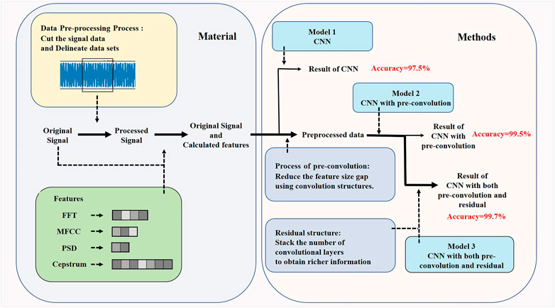
The architecture diagram for rail damage identification is shown in Figure 1.

FIGURE 1

FIGURE 1. Damage detection model architecture diagram.

2.1 Data pre-processing process

The vibration signal data used for rail damage detection in this paper was obtained from the Tianjin (China) field experimental data. The rails are processed into various damage levels, which were excited with excitation signals of 4 k, 6 k, and 10 kHz frequencies, and then the original vibration waveforms of the rails under various health conditions are collected using piezoelectric ceramic tiles. The sampling frequency was 100 kHz, and a length of 4,000 data points was selected as the step size to cut the signal data for subsequent calculation of four different signal characteristics. A total of 12,987 samples were generated, and the samples were disrupted and split into the ratio of 6:2:2 to ensure the randomness of the samples. The final number of samples in the training set was 7,793, and the number of samples in both the validation and test sets was 2,597.

2.2 Selected features

The time-domain analysis method of vibration signals shows the variation of the signal with time, which is simple and easy to operate. Frequency-domain analysis is also a common method in signal analysis. For a complex signal acquired, if analyzed from the perspective of the signal waveform, it can be considered as a superposition of several sine waves of different frequencies. The frequency-domain analysis method describes the amplitude distribution of sine waves of each frequency at a static point in time. In this paper, the Fast Fourier Transform (FFT), Mel-Frequency Cepstral Coefficients (MFCC), Power Spectral Density (PSD), and Cepstrum are selected as the features for the subsequent processing to analyze whether there is damage in the rail. These features are extracted from the original signals based on both time and frequency domain analysis methods.

2.2.1 Fast fourier transformation

The Discrete Fourier Transform (DFT) is widely used in the analytical processing of signals as a mainstream algorithm for frequency domain analysis (Sorensen et al., 1987). The Fourier transform can convert a time-domain signal into a frequency-domain signal. As shown in Eq. 1, by the idea of discrete Fourier transform, we can decompose any segment of the signal into the form of a sum of several basis functions from the perspective of multiple frequency components. The physical meaning of this decomposition is expressed as a projection of the original function onto each set of base functions.

$\mathit{X}\left(\mathit{k}\right)=\mathit{F}\left[\mathit{x}\left(\mathit{n}\right)\right]={\displaystyle \sum }_{\mathit{n}=\mathbf{0}}^{\mathit{N}-\mathbf{1}}\mathit{x}\left(\mathit{n}\right){\mathit{e}}^{-\frac{\mathit{j}2\mathit{\pi }\mathit{k}\mathit{n}}{\mathit{N}}}(1)$

The FFT is a fast algorithm for the DFT that is based on a recursive partitioning algorithm that requires only half of the operations for each calculation to produce the results for the entire sequence. The algorithmic process of FFT can be simplified as the butterfly operation shown in Figure 2 is performed continuously on the parity sequence to complete the conversion of the signal from the time-domain to the frequency-domain. Each butterfly operation requires only one plural multiplication and two plural additions.

FIGURE 2

FIGURE 2. Butterfly operation in Fast Fourier Transform.

The total number of operations of DFT and FFT is shown in Eqs 2, 3. It is obvious from the equation that the number of computations of FFT is much less than that of DFT, so using FFT can reduce the computation time and thus improve the speed of feature extraction.

${\mathit{A}}_{\mathit{D}\mathit{F}\mathit{T}}={\mathit{N}}^{\mathbf{2}}+\mathit{N}\left(\mathit{N}-\mathbf{1}\right)(2)$

${\mathbf{A}}_{\mathit{F}\mathit{F}\mathit{T}}=\left(\mathit{N}/\mathbf{2}\right){\mathbf{log}}_{\mathbf{2}}\mathit{N}+\mathit{N}{\mathbf{log}}_{\mathbf{2}}\mathit{N}(3)$

Due to the symmetry of the FFT results, we usually use half of the resulting data, which results in a 1 × 2,000 feature vector for each sample in this paper after the FFT transform.

2.2.2 Mel-frequency cepstral coefficients

Davies and Mermelstcin proposed the Mel frequency based on the auditory properties of the human ear. Mel frequency is in nonlinear correspondence with frequency. As shown in Eq. 4, Mel-frequency cepstrum coefficients are the frequency spectrum features calculated by this nonlinear relationship. Mel cepstrum is mainly applied to feature extraction and dimensionality reduction of waveform data.

${\mathit{f}}_{\mathit{M}\mathit{e}\mathit{l}}=\mathbf{1125}\times \mathit{ln}\left(\mathbf{1}+\frac{\mathit{f}}{\mathbf{700}}\right)(4)$

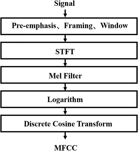
As shown in Figure 3, MFCC generally goes through the following steps: Pre-emphasis is used to amplify the high frequencies to balance the spectrum, thus avoiding numerical problems in the Fourier transform in the subsequent process and improving the noise ratio of the signal. The frequency of the signal changes with time. Assuming that the signal is fixed for a short time, the framing operation makes the Fourier transform on short frames and then concatenates adjacent frames to reduce the effect of non-stationary time variation. Windowing is the operation of adding a Hamming window, for example, to each frame after splitting it (Song and Peng, 2008). One of the main purposes of adding windows is to counteract the spectral leakage caused by the FFT calculation. The final Short Time Fourier Transform (STFT) is performed on each frame. The Mel filter bank consists of several triangular filters, and the frequency-domain signal obtained after the STFT is fed into the Mel filter bank to calculate the energy value. Since our perception of sound is not linear, a logarithmic operation is performed on the energy during the calculation. Finally, since the filter bank coefficients tend to be highly correlated due to calculations that can be transformed into each other, in order to solve the problems this correlation brings to machine learning training, it is generally eliminated by using the Discrete Cosine Transform (DCT). In this paper, the obtained 1 × 320 vector is used as the MFCC feature of the original vibration signal by the above process.

FIGURE 3

FIGURE 3. MFCC calculation flow.

2.2.3 Power spectral density

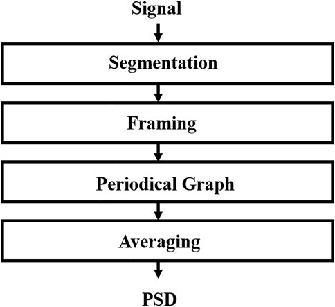
The power spectrum is also known as the power spectral density. The power spectrum is used to describe the distribution of signal power over the frequency spectrum, as the signal power varies with frequency in the unit frequency band. The power spectrum contains some of the same dimensional information as the frequency spectrum, while discarding the phase information, generally using frequency as the horizontal coordinate and power as the vertical coordinate. The area of the image is numerically equal to the energy of the signal, so the power spectrum is analyzed from the energy perspective of the signal. The calculation of power spectrum is mainly divided into two methods. The first is the autocorrelation coefficient method, and the second is the direct method, also known as the average periodogram method. In this paper, Welch’s method is chosen. Welch’s method is a modified average periodogram method, which allows the signal to overlap segments, which allows the before-and-after correlation of the data to be preserved. The signal is then windowed and then the average periodogram is calculated, and the process is shown in Figure 4. The Welch method solves the problem that the length of the data produces increased fluctuation of the spectral curve and poor resolution when using the average periodogram method to process the data. In this paper, the 1 × 129 eigenvectors calculated by the Welch method are used as the PSD features of the original vibration signal.

FIGURE 4

FIGURE 4. PSD calculation process.

2.2.4 Cepstrum

The essence of the cepstrum analysis is to take the logarithm of the power spectrum and then perform the spectrum analysis. The advantage of this is that the signal is introduced into the inverse spectrum domain, and the periodic structure and components of the spectrum can be analyzed and extracted in the new time domain. The cepstrum is better for the analysis of the periodic structure of the complex spectrum, and the requirements for the location and transmission of the sensor measurement points are small. For different location sensors, the power spectrum is not the same due to the difference in transmission paths, and the cepstrum can distinguish the effects transmitted in the vibration domain. Thus, in the process of cepstrum analysis, it is not necessary to consider the effect brought on by the signal measurement. The signal cepstrum is calculated as follows:

1) Fourier transform any time series signal X (t) to obtain X (f).

$\mathit{X}\left(\mathit{f}\right)=\mathit{F}\mathit{F}\mathit{T}\left[\mathit{X}\left(\mathit{t}\right)\right](5)$

2) The power spectrum is obtained by squaring X (f).

${\mathit{S}}_{\mathit{x}\mathit{x}}\left(\mathit{f}\right)={\mathit{X}}^2\left(\mathit{f}\right)(6)$

3) Inverse Fourier transform of the power spectrum of the vibration signal by taking the logarithm.

${\mathit{C}}_{\mathit{x}\mathit{x}}\left(\mathit{t}\right)=\mathit{F}\mathit{F}{\mathit{T}}^{-\mathbf{1}}\left[\mathbf{10}\mathit{l}{\mathit{g}}_{\mathit{x}\mathit{x}}\left(\mathit{f}\right)\right](7)$

In this paper, the calculated 1 × 4,000 vector is used as the cepstrum feature of the original vibration signal.

2.3 Proposed models

2.3.1 CNN architecture

CNN is a kind of neural network that contains convolutional computation and has a certain depth structure (Ma et al., 2021). With the proposal of deep learning theory and the continuous progress of computer hardware equipment, it is widely used in various injury detection tasks, which can predict the injury condition quickly and accurately. The input of the CNN model in this paper consists of the original vibration signal data and four features extracted by FFT, MFCC, power spectrum, and cepstrum, where the calculated length of the original vibration signal is 4,000, and the calculated length of the features from FFT, MFCC, power spectrum, and cepstrum are 2,000, 320, 129, and 4,000, respectively. Since discrepant data can cause numerical problems in the training process of neural networks, in order to speed up the process of gradient descent and give meaning to the two-dimensional convolution of the data, this paper first normalizes the original data and the four features are computed as shown in Eqs 8, 9.

${\mathit{x}}^{\prime }=\frac{\mathit{x}-{\mathit{x}}_{\mathit{m}\mathit{e}\mathit{a}\mathit{n}}}{{\mathit{x}}_{\mathit{s}\mathit{t}\mathit{d}}}(8)$

$\mathit{x}=\left({\mathit{x}}^{\prime }{\mathit{x}}_{\mathit{s}\mathit{t}\mathit{d}}+{\mathit{x}}_{\mathit{m}\mathit{e}\mathit{a}\mathit{n}}\right)\times \mathbf{256}(9)$

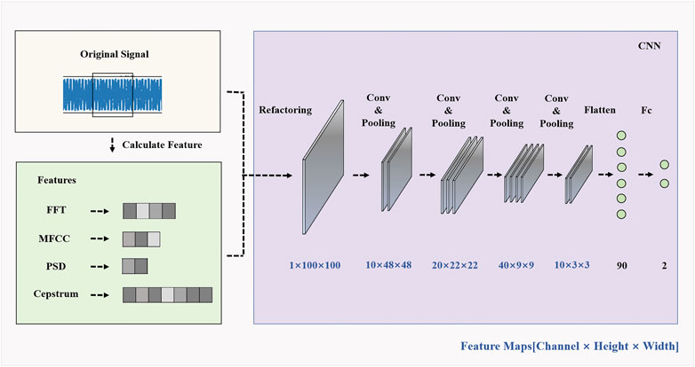
Here the result is expanded 256 times in order to give the data similar information as a grayscale map. Then the five features are stitched horizontally and then reconstructed into a 100 × 100 two-dimensional grayscale information map. After a 4-layer convolutional structure as shown in Figure 5, the dichotomous data is obtained through the fully connected layer as the output result for determining whether there is damage in the rails.

FIGURE 5

FIGURE 5. CNN architecture.

2.3.2 CNN with pre-convolution

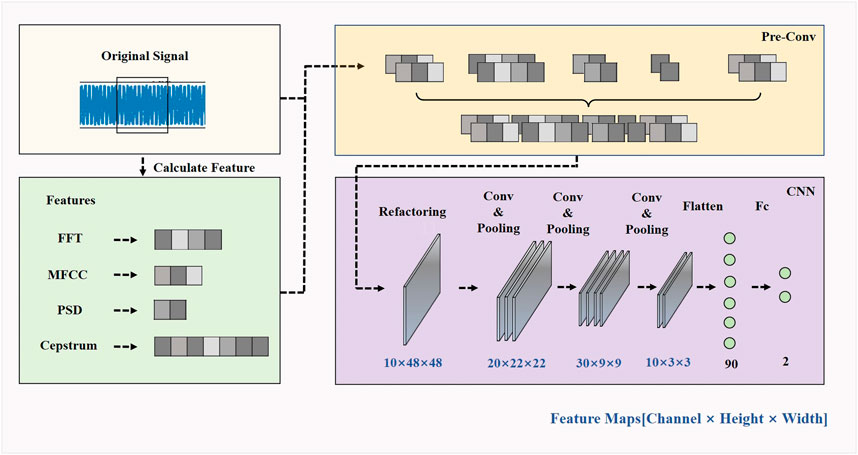
For the above-mentioned CNN, we note that the size of the features computed by the traditional theoretical method varies, and the direct stitching of the features will make the features with larger sizes have larger weights in the training process of the neural network, thus diluting the effect of the features with smaller sizes. To address the above problem, we adopt a pre-convolution processing method to improve the CNN by referring to the idea of FCN.FCN makes it possible to input features of different sizes into the same network by replacing the fully connected layer in CNN with a convolutional layer (Long et al., 2015). The difference between the two is that convolution is a local connection while full connection is a global connection. In fact, for full connection, the last feature map is equivalent to a full connection of convolutional kernel size if it is not expanded and the output dimension is directly used instead. The concepts of maximum local and global are actually equivalent, and thus a convolutional layer can be used instead of a fully connected layer. As shown in Figure 6, in a traditional CNN architecture, if a 14 × 14 image is convolved, the first 2 layers are the convolution and pooling layers, and the 3rd and 4th layers stretch the result of convolution into a one-dimensional vector of length 2, which is thus used as the prediction result for classification. FCN replaces these two layers with a convolution layer, which allows the convolution kernel to slide over the image and convolve in steps, regardless of the size of the input image. If the size of the convolution kernel is set to the same size as the upper image, as shown in the figure, the first layer is convolved with a convolution kernel with 4 channels and a width of 5 and a height of 5, and the second layer is convolved with a convolution kernel with 2 channels and a width of 1 and a height of 1, the final probability of binary classification is obtained. This result is consistent with the use of a fully connected CNN. Thus, any fully-connected layer can be converted into a convolutional layer. The advantage of using a convolutional layer instead of a fully connected layer is that it allows the convolutional network to slide over larger input images, thus breaking the limitation on the image input size.

FIGURE 6

FIGURE 6. Comparison of CNN and FCN.

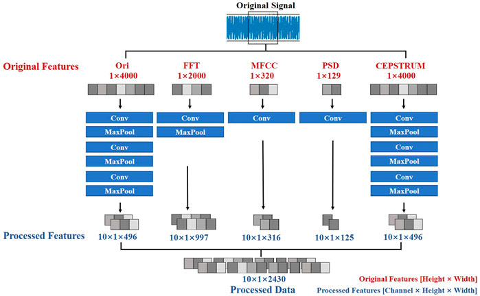
Similarly, in this paper, the calculated features with different sizes are fed into different pre-convolutional layers in order to reduce the length of the longer-sized features to fit the shorter-sized features. For one-dimensional data generated using the first-tail splicing method, the neural network is difficult to distinguish different features involved in the splicing. Therefore, the neural network generally focuses more on the features with longer sizes, which means that the longer the feature size is, the higher the weight will be used in the training process of the model. Pre-convolution is used to reduce the length of the features with longer sizes, which can solve the problem of too large a gap in the neural network’s implied weight assignment to the features with different sizes.

As shown in Figure 7, three convolution pooling nonlinear activation operations are performed on the original data by a convolution kernel of size 5. One convolution pooling and nonlinear activation are performed on the FFT calculation results. Three convolution pooling and nonlinear activation operations are performed on the power cepstrum calculation results. Only one convolution operation of size 5 is performed on the power spectral density and MFCC. The convolution results are subsequently stitched horizontally and reconstructed into a 10-channel 48 × 48 grayscale information map as the input to the subsequent CNN.

FIGURE 7

FIGURE 7. Process of pre-convolution.

The specific process of CNN with pre-convolution is shown in Figure 8. After normalizing the input raw data and the computed four features and expanding the result by 256 times, the result is reconstructed into a two-dimensional grayscale map by splicing the first and the last as the input of the CNN, so that the CNN captures the feature information of the grayscale map in the same way as processing the image. The data is reconstructed into a 10-channel 2D matrix after the pre-convolution process, and the CNN is made to capture the complex grayscale map information through the convolution kernel by increasing and decreasing the number of channels in the process. After pre-convolution, the first layer uses 20 convolution kernels of size 4, and the pooling layer uses a maximum pooling of 2 × 2, and then the result dimension is 20 × 22 × 22 after nonlinear activation. The second layer uses 30 convolution kernels of size 4, and the output dimension is 30 × 9 × 9 after the same pooling and activation. The third layer uses 10 convolution kernels of size 4, and the output dimension is 10 × 3 × 3 after pooling and activation. The final convolution result is then passed through two fully connected layers to obtain the binary prediction result.

FIGURE 8

FIGURE 8. CNN with pre-convolution.

2.3.3 CNN with both pre-convolution and residual structures

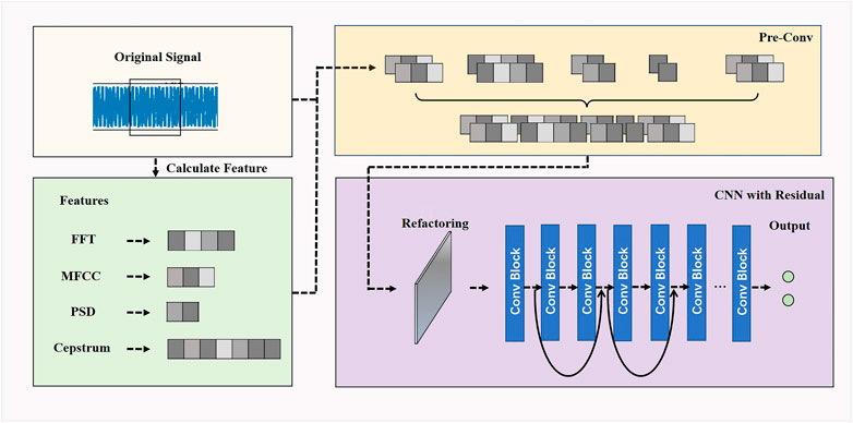
For a general network architecture, increasing the number of convolutional layers can make the neural network extract richer features and thus improve the accuracy of the model; but in fact, the more convolutional layers, the more nonlinear layers will be stacked, which makes the model’s nonlinear fitting ability too strong and leads to a decrease in the accuracy of the model (He et al., 2016). We hope to still use a relatively simple architecture like CNN to obtain higher accuracy while keeping the model lightweight and to make the training converge faster in order to extract richer features to help improve its performance in damage recognition. Residual neural network (Resnet) is a kind of convolutional neural network that introduces a residual structure, which allows us to stack the number of convolutional layers to form a network with relatively more convolutional blocks, which enables us to obtain richer information. At present, Resnet performs very well in various tasks in the field of computer vision. Figure 9 shows the architecture of a CNN using pre-convolution processing while introducing the residual structure.

FIGURE 9

FIGURE 9. CNN with both pre-convolution and residual.

The architecture of the CNN with residuals structures is shown in Figure 10. In this paper, based on the lightweight CNN architecture, the number of convolutional layers is increased by means of residual connections, and finally a CNN with both pre-convolution and residual is built.

FIGURE 10

FIGURE 10. CNN with residual.

3 Results and discussion

The training results of the three networks on our dataset are shown in Figure 11. Figure 11A represents the performance of the normal CNN performing 50 epochs on both the training and validation sets. Through testing on the test set, the normal CNN is finally verified to have 97.9% classification accuracy. Figure 11B shows the results of the CNN with pre-convolution performing 40 epochs on both the training and validation sets, which shows that the convergence of the model training is accelerated and the accuracy on both the training and validation sets is improved with the pre-convolution processing. The test results on the test set show that the network architecture with pre-convolution improves the accuracy from 97.9% to 99.5% with fewer training rounds. Figure 11C shows the performance of the CNN with both pre-convolution and residual on the training and validation sets. It can be seen that the convergence speed of the model training with the residual structure is further improved compared to the above two types of CNNs, and the results of the test set show that the accuracy of the model has been stabilized at 99.7% after only 15 rounds of training, which is more advantageous than the other two models in the rail damage detection task.

FIGURE 11

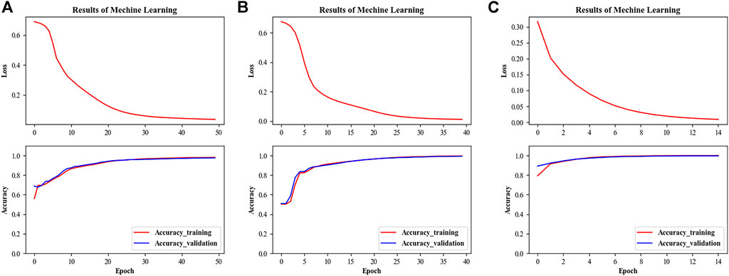
FIGURE 11. Comparison of the training results of the three networks. (A) CNN (B) CNN with pre-convolution (C) CNN with both pre-convolution and residual.

In addition to comparing the loss and accuracy of the networks, we can also visualize the classification performance of the three neural network models on positive and negative samples by introducing the confusion matrix (Ma et al., 2021). The confusion matrix, also known as the error matrix, can be used to judge whether a classifier is good or not. As shown in Figure 12A, from the confusion matrix, we can visualize that among the tested samples, the CNN without the pre-convolution predicts a total of 20 true lossless samples as lossy and a total of 34 true lossy samples as lossless. By comparing the confusion matrix in Figure 12B, it can be seen that the use of the pre-convolution structure and the multi-feature association approach substantially reduces the number of misclassifications in both categories on the same test set. As Figure 12C shows the confusion matrix calculated on the test set for the CNN using the residual structure and pre-convolution processing, we can see that the probability of drawing incorrect conclusions is further reduced for the network using the residual structure.

FIGURE 12

FIGURE 12. Comparison of the confusion matrices obtained from the three network models computed on the test set. (A) CNN (B) CNN with pre-convolution (C) CNN with both pre-convolution and residual.

In addition to analyzing the positive and negative sample classification performance from the confusion matrix, we also calculated and analyzed other classification performance metrics of the model. Using the confusion matrix and the experimental data, True Positive (TP), False Positive (FP), False Negative (FN), and True Negative (TN) can be calculated. Where TP means a lossy data is correctly predicted as lossy by the model, FP means a lossless data is predicted as lossy, FN means a lossy data is predicted as lossless by the model, TN means a lossless data is predicted as lossless. TP and TN represent the fraction predicted correctly by the network, while FN and FP represent the fraction predicted incorrectly by the network. The Precision Rate indicates the proportion of samples with positive predictions to the total number of samples with correct predictions. The Recall Rate indicates the proportion of samples with positive predictions to all positive samples. The F1 Score is the summed average of the precision and recall rates and is a measure of the accuracy of a binary classification model that takes into account both precision and recall rates. Matthews Correlation Coefficient (MCC) is a balanced measure of the classification performance of binary classification, which considers the true results as two 0–1 distributions; MCC = 1 when FP = FN = 0 and MCC = −1 when the prediction is completely wrong. = −1. The formula for the above classification performance metric is shown in Eqs 10–13.

$\mathit{P}\mathit{r}\mathit{e}\mathit{c}\mathit{i}\mathit{s}\mathit{i}\mathit{o}\mathit{n}=\frac{\mathit{T}\mathit{P}}{\mathit{T}\mathit{P}+\mathit{F}\mathit{P}}(10)$

$\mathit{R}\mathit{e}\mathit{c}\mathit{a}\mathit{l}\mathit{l}=\frac{\mathit{T}\mathit{P}}{\mathit{T}\mathit{P}+\mathit{F}\mathit{N}}(11)$

$\mathit{F}\mathbf{1}=\frac{\mathbf{2}\mathit{T}\mathit{P}}{\mathbf{2}\mathit{T}\mathit{P}+\mathit{F}\mathit{P}+\mathit{F}\mathit{N}}(12)$

$\mathit{M}\mathit{C}\mathit{C}=\frac{\mathit{T}\mathit{P}\times \mathit{T}\mathit{N}-\mathit{F}\mathit{P}\times \mathit{F}\mathit{N}}{\sqrt{\left(\mathit{T}\mathit{P}+\mathit{F}\mathit{P}\right)\left(\mathit{T}\mathit{P}+\mathit{F}\mathit{N}\right)\left(\mathit{T}\mathit{N}+\mathit{F}\mathit{P}\right)\left(\mathit{T}\mathit{N}+\mathit{F}\mathit{N}\right)}}(13)$

Table 1 shows the classification performance evaluation metrics for the three models used in our evaluation, where the precision rate represents the percentage of samples predicted to be injured or damaged that actually have damage, and it is used to measure the ability of the model to avoid errors. The data in the table shows that the use of pre-convolution and the introduction of the residual structure successfully improved the precision rate of our model. Only 0.003% of the samples predicted to be injured were misclassified as damaged by the model, demonstrating a high confidence level if the samples were predicted to be damaged by the model. The recall rate in our injury detection task indicates the proportion of samples predicted as damaged to the true damaged in the test set, which is used to measure the model’s ability to find damaged samples. The data in the table shows that CNN with both pre-convolution and residual also has a high recall rate, as shown by the fact that our model found 99.7% of the injury samples on the test set and only 0.003% of the injury samples were not found, which indicates that our model has a good ability to find injury samples. F1 score and MCC are two combined metrics that combine precision and recall. Precision and recall are contradictory variables. If we increase the precision rate and only determine injury for samples that we are confident are injured, then the recall rate will be lower, and if we determine injury as much as possible to increase the recall rate, then the precision rate will be lower. We want the prediction of damage to be as accurate as possible, thus avoiding the waste of resources by testing the damage a second time. At the same time, we want the recall rate to be very high because the danger of missing detection is very high and may cause serious losses. The F1 score and MCC show that our model still has good performance when considering both accuracy and recall. The use of pre-convolution and the introduction of residual structure both improve the F1 score and MCC, and the F1 score and MCC of CNN with both pre-convolution and residual reach 0.997 and 0.995, respectively.

TABLE 1

TABLE 1. Comparison of model metrics.

4 Conclusion

Damage detection of the rails is of great significance for railroad safety. In this paper, a vibration signal-based detection method is proposed. Traditional theoretical research methods are used to calculate the features of vibration signals as the inputs of deep learning models. The presence of potential rail damage in the vibration signal is predicted using CNN. The three different convolutional network architectures are finally compared, and their performance in rail damage detection is tested on our experimentally measured dataset. The results show that the CNN with both pre-convolution and Residual structures achieves the accuracy of 99.9%, which is better than the other two network architectures. At the same time, the vibration signal-based CNN model is safer, more energy-efficient and more conventional, which is more in line with modern large-scale rail damage detection needs.

Data availability statement

The raw data supporting the conclusion of this article will be made available by the authors, without undue reservation.

Author contributions

ZZ: conceptualization; early draft; methodology; writing-review and editing. YS: conceptualization; curation; feedback; writing-review and editing; funding acquisition. XC: discussion extension; feedback; writing-review and editing.

Funding

This research was funded by the National Natural Science Foundation of China (92067110).

Acknowledgments

We thank the Research Project on Multidimensional Data Characterization Methods and Structured Organization Mechanisms of Production Factors of Shenyang Institute of Automation Chinese Academy of Sciences (Grant No. 92067110) for supporting this topic.

Conflict of interest

The authors declare that the research was conducted in the absence of any commercial or financial relationships that could be construed as a potential conflict of interest.

Publisher’s note

All claims expressed in this article are solely those of the authors and do not necessarily represent those of their affiliated organizations, or those of the publisher, the editors and the reviewers. Any product that may be evaluated in this article, or claim that may be made by its manufacturer, is not guaranteed or endorsed by the publisher.

References

Cheng, L., Li, G., Nie, Z., and Ma, H. (2010). “Visualization research of damage detection in rail,” in 2010 Proceedings of the Third International Symposium on Information Processing (ISIP 2010), Qingdao, Shandong China, Oct. 15 2010 to Oct. 17 2010, 502–505. doi:10.1109/isip.2010.145

CrossRef Full Text | Google Scholar

Flah, M., Nunez, I., Ben Chaabene, W., and Nehdi, M. L. (2020). Machine learning algorithms in civil structural health monitoring: A systematic review. Arch. Comput. Methods Eng. 28 (4), 2621–2643. doi:10.1007/s11831-020-09471-9

CrossRef Full Text | Google Scholar

Han, Q., Liu, J., Feng, Q., Wang, S., and Dai, P. (2021). Damage detection method for rail surface based on multi-level feature fusion. China Railw. Sci. 42 (5), 41–49.

Google Scholar

Han, S. W., Cho, S. H., Jang, G. W., and Park, J. H. (2015). Non-contact inspection of rail surface and internal defects based on electromagnetic ultrasonic transducers. J. Intelligent Material Syst. Struct. 27 (3), 427–434. doi:10.1177/1045389x15610910

CrossRef Full Text | Google Scholar

He, K. M., Zhang, X. Y., Ren, S. Q., and Sun, J. (2016). “Deep residual learning for image recognition,” in 2016 IEEE Conference on Computer Vision and Pattern Recognition (CVPR), NEW YORK, June 27 2016 to June 30 2016, 770–778.

CrossRef Full Text | Google Scholar

Lei, Y. G., Yang, B., Jiang, X. W., Jia, F., Li, N. P., and Nandi, A. K. (2020). Applications of machine learning to machine fault diagnosis: A review and roadmap. Mech. Syst. Signal Process. 138, 106587. doi:10.1016/j.ymssp.2019.106587

CrossRef Full Text | Google Scholar

Li, Y. J., Yao, F. T., Jiao, S. B., Huang, W. C., and Zhang, Q. (2020). “Identification and classification of rail damage based on ultrasonic echo signals,” in 39th Chinese Control Conference (CCC), NEW YORK, 27-29 July 2020, 3077–3082.

Google Scholar

Liang, B., Iwnicki, S. D., Zhao, Y., and Crosbee, D. (2013). Railway wheel-flat and rail surface defect modelling and analysis by time–frequency techniques. Veh. Syst. Dyn. 51 (9), 1403–1421. doi:10.1080/00423114.2013.804192

CrossRef Full Text | Google Scholar

Long, C. S., and Loveday, P. W. (2013). “Prediction of guided wave scattering by defects in rails using numerical modelling,” in 10th International Conference on Barkhausen and Micro-Magnetics (ICBM), MELVILLE, 21/07/13→26/07/13, 240–247.

Google Scholar

Long, J., Shelhamer, E., and Darrell, T. (2015). “Fully convolutional networks for semantic segmentation,” in IEEE Conference on Computer Vision and Pattern Recognition (CVPR), Boston, MA, USA, 7-12 June 2015, 3431–3440.

CrossRef Full Text | Google Scholar

Lu, J., Liang, B., Lei, Q., Li, X., Liu, J., Liu, J., et al. (2020). SCueU-Net: Efficient damage detection method for railway rail. IEEE Access 8, 125109–125120. doi:10.1109/access.2020.3007603

CrossRef Full Text | Google Scholar

Ma, L. B., Li, N., Guo, Y. N., Wang, X. W., Yang, S. X., Huang, M., et al. (2021). Learning to optimize: Reference vector reinforcement learning adaption to constrained many-objective optimization of industrial copper burdening system. IEEE Trans. Cybern. 14, 1. doi:10.1109/tcyb.2021.3086501

CrossRef Full Text | Google Scholar

Ma, L., Wang, X., Wang, X., Wang, L., Shi, Y., and Huang, M. (2021). Tcda: Truthful combinatorial double auctions for mobile edge computing in industrial internet of things. IEEE Trans. Mob. Comput. 2021, 1. doi:10.1109/tmc.2021.3064314

CrossRef Full Text | Google Scholar

Song, Y. Z., and Peng, X. (2008). “Spectra analysis of sampling and reconstructing continuous signal using hamming window function,” in 4th International Conference on Natural Computation (ICNC 2008), NW Washington, DC United States, October 18 - 20, 2008, 48–52.

CrossRef Full Text | Google Scholar

Sorensen, H. V., Jones, D. L., Heideman, M. T., and Burrus, C. S. (1987). Real-valued fast fourier-transform algorithms. IEEE Trans. Acoust. 35 (6), 849–863. doi:10.1109/tassp.1987.1165220

CrossRef Full Text | Google Scholar

Suwansin, W., and Phasukkit, P. (2021). Deep learning-based acoustic emission scheme for nondestructive localization of cracks in train rails under a load. Sensors 21 (1), 272. doi:10.3390/s21010272

CrossRef Full Text | Google Scholar

Thomas, H. M., Heckel, T., and Hanspach, G. (2007). Advantage of a combined ultrasonic and eddy current examination for railway inspection trains. Insight - Non-Destructive Test. Cond. Monit. 49 (6), 341–344. doi:10.1784/insi.2007.49.6.341

CrossRef Full Text | Google Scholar

Tian, L. L., Wang, Z. D., Liu, W. B., Cheng, Y. H., Alsaadi, F. E., and Liu, X. H. (2021). A new GAN-based approach to data augmentation and image segmentation for crack detection in thermal imaging tests. Cogn. Comput. 13 (5), 1263–1273. doi:10.1007/s12559-021-09922-w

CrossRef Full Text | Google Scholar

Wilson, J., Tian, G. Y., Mukriz, I., and Almond, D. (2011). PEC thermography for imaging multiple cracks from rolling contact fatigue. Ndt E Int. 44 (6), 505–512. doi:10.1016/j.ndteint.2011.05.004

CrossRef Full Text | Google Scholar

Xu, L., Chen, X. M., Xu, W. C., Li, X. J., Meng, X. H., and Tang, Y. K. (2014). Application of wavelet energy spectrum in railway track detection. J. Vib. Eng. 27 (4), 605–612.

Google Scholar

Xu, Q. H., Zhao, Q. J., Yu, G., Wang, L. G., and Shen, T. (2020). “Rail defect detection method based on recurrent neural network,” in 39th Chinese Control Conference (CCC), 27-29 July 2020, Shenyang, China, 6486–6490.

CrossRef Full Text | Google Scholar

Yuan, Z., Zhu, S., Yuan, X., and Zhai, W. (2021). Vibration-based damage detection of rail fastener clip using convolutional neural network: Experiment and simulation. Eng. Fail. Anal. 119, 104906. doi:10.1016/j.engfailanal.2020.104906

CrossRef Full Text | Google Scholar

Zhang, X., Zou, Z. X., Wang, K. W., Hao, Q. S., Wang, Y., Shen, Y., et al. (2018). A new rail crack detection method using LSTM network for actual application based on AE technology. Appl. Acoust. 142, 78–86. doi:10.1016/j.apacoust.2018.08.020

CrossRef Full Text | Google Scholar

Zhao, C., Wang, P., Quan, S., Cao, Y., and Hu, G. (2012). Detection method for broken rail based on rate of change of strain mode. J. Vib. Meas. Diagnosis 32 (5), 723–729.

Google Scholar