 Congcong Li
 Chaoqiang Fang2
 Hailong Zuo
 Shuoliang Wang
95% of researchers rate our articles as excellent or good
Learn more about the work of our research integrity team to safeguard the quality of each article we publish.
Find out more
METHODS article
Front. Energy Res. , 16 November 2022
Sec. Process and Energy Systems Engineering
Volume 10 - 2022 | https://doi.org/10.3389/fenrg.2022.1005749
A significant amount of bypassed oil resources often remain in a mature waterflooding reservoir because of non-uniform sweep caused by natural complexities of a subsurface reservoir and improper management of the reservoir. Infill drilling is one of the most attractive options for increasing oil recovery in consequence of its operational simplicity, low risk and promising results. Determining optimal infill well placements in heterogeneous mature reservoirs is a critical and challenging task that has a significant impact on the recovery performance and economic revenue of subsurface remaining oil resources. An integrated framework is constructed to attain best-obtained optimal location and completion of infill wells in multi-layer mature oil reservoirs. The placement of an infill vertical well is parameterized in terms of two sets of variables that define the location and completion respectively. A variant of SPSA algorithm is used to solve the defined optimization problem. The performance of the proposed algorithm is first tested for the joint optimization of well location and completion of an injection well using a synthetic model. The results show that the algorithm with average SPSA gradients outperforms the single SPSA gradient method both in solution and convergence rate. Besides, there are two plateaus on the performance curve of all algorithms: on the first plateau, each algorithm is approaching to its optimal well location with relatively little change on the completion parameters, while on the second plateau, each algorithm obtains the corresponding optimal completions. A complex heterogeneous reservoir model is then constructed by using the data of a mature oil reservoir in Shengli Oilfield in China to design an optimal 10 years’ infill drilling program. Four vertical production wells are placed in the oil-rich regions and both simultaneous and sequential algorithms are tried to obtain their optimal locations and completions. The performances of simultaneous joint optimization and sequential joint optimization are compared and as a result it is recommended to use sequential joint optimization as the optimization algorithm in the integrated framework.
About 92% of oil reservoirs in China are characterized by continental clastic sediments with complex vertical and lateral heterogeneities and high levels of crude oil viscosity (Han, 2010). Waterflooding with uniformly spaced well pattern has always been the main development approach for Chinese oilfields. After decades of producing, most of the major oilfields have entered the late stage of waterflooding life cycle featured by high water-cut (greater than 80%) and high recovery of recoverable reserves (greater than 70%). Although most of mature oilfields are encountering such terrible situations, they still contribute to a great proportion of crude oil supply in China. According to official statistics, more than 70% of the total national oil production are from mature oilfields at present (Han, 2010). Production practice shows that there still is a great potential to improve the recovery of high water-cut oilfields. The decreasing trend in discovering new conventional hydrocarbon resources is necessitating optimal recovery from existing reserves in a more cost-effective manner.
Due to strong reservoir heterogeneities, the remaining oil distribution generally presents a feature of “highly scattered on the whole and relatively abundant in local areas” when the comprehensive water-cut in oilfields is beyond 80% (Han, 2007). The two major methods to improve water sweep efficiency that were once applied effectively at lower water-cut stage, including subdivision of development intervals and uniform infilling wells, began to show little or even no effects. This is mainly because the achievements of the above methods at lower water-cut stage of development are owed to the large-area distributions of remaining oil in relatively low-to-moderate permeability layers at that time, but the current condition becomes very different in that the overall remaining oil is highly scattered even in low-to-moderate permeability layers. In this case, uniform infilling wells are not as efficient as before. The initial water-cut in most newly drilled infilling wells can be as high as 80% and few even higher than 90% (Han, 2010). In order to further improve the recovery of remaining oil reserves, it needs to drill individualized infill wells rather than uniform infill wells.
Determining appropriate well placements of producers and injectors is an important aspect of overall development strategy of any field. Well placement optimization becomes particularly noteworthy in mature oilfields where an enormous amount of pore volumes are occupied by water and both reservoir geological characteristic and remaining oil distribution are extremely complex. Thus, new wells have to be drilled based on a comprehensive understanding of reservoir description. In Chinese mature oilfields, each wellbore may penetrate many prospective reservoir layers that can range, depending on the field size and number of reservoirs, from a few into the hundreds. However, technical and reservoir management considerations usually make every wellbore capable of producing from only a limited completion interval. The region that an infill well to be located in, the reservoir layer to be penetrated and the length of the perforated or open section of a well will together influence the development performance greatly. Hence, the main objective of infill well placement optimization should be optimizing not only the areal drainage pattern but also the vertical scheme. Optimizing both well location and perforation along formation intervals could help maximize the control reserve of a single well, homogenize the inflow-velocity profile and prevent early water breakthrough and rapid water-cut increase in high-permeability completion intervals, which are all critically important for enhancing oil recovery and improving economic revenue of mature oilfields. However, there could be a large number of possible candidate locations for a new well. To search through and evaluate all the possible locations is not practically feasible, particularly for high resolution geologic models consisting of multimillion cells. For large scale field applications, a practical method is needed to mitigate the computational burden associated with the possibly large number of simulation runs.
Traditionally, optimization of well placement has been done by using quality maps that indicate which regions of the reservoir have not been adequately swept by the injected water (Badru, 2003; Kharghoria et al., 2003; da Cruz et al., 2004; Guimaraes et al., 2005; Taware et al., 2012). The quality maps are typically based on static properties such as permeability, porosity, structure and net thickness, and dynamic properties such as remaining oil, pressure, well productivity and cumulative oil production. Although this method is convenient for application, it cannot properly place wells in locations that take advantage of long-term high oil saturation or respond to the dynamics of reservoir fluid flow over a long period of time. Simply placing wells based on saturation or quality maps may not guarantee long term profitability of the project. In recent years, various simulation-based optimization techniques have also been introduced to automate the process of attaining the optimal well locations. There are many challenges in the field of automatic well placement optimization, such as variable design, objective function, constraints formulation, optimization algorithm, geological uncertainty, computational cost and so on. We will just discuss a few of them for brevity in this paper.
One important aspect of automatic well placement approaches is the description of well location and/or well trajectory. As for well placement problem, the actual physical problem of determining well location and trajectory is a continuous problem, while the completions of a well in the formation are commonly introduced into the numerical simulation model as integral indices of the connected gridblocks. Thus, to parameterize the location and, in general the trajectory of the wells, both discrete variables (Yeten et al., 2003; Bangerth et al., 2006; Ozdogan and Horne, 2006; Emerick et al., 2009; Bellout et al., 2012; Li et al., 2013) and continuous real-valued variables (Onwunalu and Durlofsky, 2010; Bouzarkouna et al., 2012; Forouzanfar et al., 2012; Forouzanfar and Reynolds, 2013; Nwankwor et al., 2013; Forouzanfar et al., 2016) are used. For a discrete optimization problem, decision variables are well connection gridblock indices. The center point of the well is moved from one gridblock to another at each iteration of whatever optimization algorithm is used. For a continuous optimization problem, the well trajectory is generally parameterized in a more real but complex way, which could make the method uneasy to implement.
Another important aspect of automatic well placement approaches is the optimization algorithm. To solve the optimal well placement problem, most researchers have utilized heuristic global optimization methods such as genetic algorithm (GA) (Montes et al., 2001; Yeten et al., 2003; Ozdogan and Horne, 2006; Emerick et al., 2009; Salmachi et al., 2013), differential evolution (DE) (Afshari et al., 2015; Awotunde, 2016), simulated annealing (Sa) (Beckner and Song, 1995), particle swarm optimization (PSO) (Onwunalu and Durlofsky, 2010; Bouzarkouna et al., 2013; Afshari et al., 2014; Forouzanfar et al., 2016), the covariance matrix adaptation-evolution strategy (CMA-ES) algorithm (Bouzarkouna et al., 2012; Jesmani et al., 2016a; Forouzanfar et al., 2016) and some hybrid algorithms (Nwankwor et al., 2013). Although these methods have the ability to avoid local solutions, their convergence to the global solution is heuristic in natural and typically require a very large number of reservoir simulation runs in an optimization loop. Moreover, to account for model uncertainty, it is often need to evaluate the performance of well placements over multiple geological realizations, which makes them too computationally expensive and thus, may not be well-suited for large scale field applications. Some local search optimization algorithms were also applied to the well placement optimization problem such as gradient-based method algorithms with adjoint gradient (Wang et al., 2007; Sarma and Chen, 2008; Zandvliet et al., 2008; Vlemmix et al., 2009; Li and Jafarpour, 2012; Forouzanfar and Reynolds, 2014), methods on the basis of the simultaneous perturbation stochastic approximation (SPSA) (Bangerth et al., 2006; Li et al., 2013; Jesmani et al., 2016b), derivative-free methods (Forouzanfar et al., 2012; Forouzanfar and Reynolds, 2013; Isebor et al., 2014a; Isebor et al., 2014b) and generalized pattern search (GPS) (Bellout et al., 2012). Among these local search algorithms, gradient-based method has the superior computational efficiency. However, one must calculate the gradient of the objective function and the constraints with respect to the optimization variables to apply the efficient gradient-based method. The adjoint for computing these gradients is not commonly provided in commercial reservoir simulators, which makes the adjoint methods are difficult to implement and require access to the simulator source code.
An alternative approach to gradient-based method is the stochastic optimization method. In particular, the simultaneous perturbation stochastic approximation (SPSA) has been developed for solving large dimensional multivariate optimization problems where the gradient information is not available (Spall, 1992; Spall, 1994; Spall, 1998; Spall, 2000). Various kinds of SPSA algorithms have been successfully applied in several engineering fields. Early applications of SPSA algorithm in petroleum engineering field were performed by Bangerth et al. (Bangerth et al., 2006) and Gao et al. (Gao et al., 2007). In Bangerth et al. (Bangerth et al., 2006), a variant of SPSA (integer SPSA) is introduced to solve the well placement problem. The authors compared and analyzed the efficiency, effectiveness, and reliability of several optimization algorithms, including the simultaneous perturbation stochastic approximation (SPSA), finite difference gradient (FDG), very fast simulated annealing (VFSA) and genetic algorithm (GA), for the well placement problem by a set of numerical waterflooding experiments and found that none of these algorithms guarantees to find the optimal solution, but both SPSA and VFSA are very efficient in finding nearly optimal well locations with a high probability. In Gao et al. (Gao et al., 2007), both SPSA and adaptive SPSA are applied to the history matching problem. The authors presented modifications for improvement in the convergence behavior of the SPSA algorithm for history matching and compared its performance to the steepest descent, gradual deformation and LBFGS algorithm and concluded that although the convergence properties of the SPSA algorithm are not nearly as good as the LBFGS methods, the SPSA algorithm is not simulator specific and it can be coupled easily with any commercial reservoir simulator to do automatic history matching. Since the two primary works, the SPSA algorithm has been widely used to solve various optimization problems in petroleum engineering field (Wang et al., 2009; Li and Reynolds, 2011; Do et al., 2012; Do and Reynolds, 2013; Li et al., 2013; Jesmani et al., 2016b; Pouladi et al., 2020).
For simulation-based well placement optimization approaches, the reliability of the solution depends seriously on the main parameters defining the geological model, including formation structure, porosity and permeability distributions, and fluid contacts. Due to limited reservoir description knowledge, these parameters are all uncertain and generally described by some probability density functions. Management of the effect of geological uncertainty on well placement optimization is another research area that is gaining more and more consideration from researchers (Ozdogan and Horne, 2006; Li and Reynolds, 2011; Li et al., 2013; Chang et al., 2015; Jesmani et al., 2016b; Temizel et al., 2018). A common practical approach for taking into account the uncertainty in well placement problem is to approximate the probability distributions with multiple equally probable geological realizations, and then optimize the expected value of the objective function over an ensemble of the model realizations, namely ensemble-based optimization. To reduce the computation time associated with the optimization process, a variety of techniques have been developed to select a relatively small ensemble of model realizations, as the representatives of all possible realizations. A fit-for-purpose sampling selection procedure is preferred, as it in general can guarantee to capture the underlying uncertainty by using as few samples as possible.
Although there is a significant advancement on the subject of well placement optimization in the last decades, few have been done to consider the effect of perforation scheme in multiply layers with different reservoir properties and oil distributions. This work presents a methodology for joint optimization of infill well location and completion using a variant of SPSA algorithm. Our optimization algorithm is an extension of the work by Bangerth et al. (Bangerth et al., 2006). We follow Bangerth et al. (Bangerth et al., 2006) to apply a bounding operator and a rounding operator to handle inequality constraints and the integer problem of well location variables, respectively. However, additional treatments to the particular problem presented in this study are also conducted. A parameter scaling handling process is implemented to eliminate the impact of different ranges of optimizing variables since we solve a joint optimization problem. Besides, we use average stochastic gradient calculated by multiply random sampling of perturbation vectors to improve the estimation of the search direction. We also introduce a simple line search procedure and a blocking step to guarantee the convergence and stability of the algorithm.
The paper is organized as follows: Section 2 presents the basic components that are used for the solution of the well placement problem, including the formulations describing the optimization problems and the objective function; Section 3 illustrates the methodology for solving the combined well location and completion optimization problem based on SPSA algorithm and the framework for coupling the reservoir flow simulator and the optimization algorithm; Section 4 presents the validation of the proposed method by using a synthetic model and its application on optimization of an infilling plan for a mature oilfield in China; Section 5 summarizes the results of the presented work and discusses possible directions of further research.
The problem considered in this work is to determine the optimal location and completion of infill wells to maximize oil recovery and profits for mature waterflooding reservoirs in the future. Numerical simulations are conducted using a commercial reservoir simulator (Eclipse E100 (GeoQuest, 2018)) to evaluate the performance of the reservoir under different well configurations.
We consider the placement of a vertical well in a heterogeneous multi-layer reservoir. The wellbore is assumed to have one or several completion/perforation intervals. Figure 1 is the typical schematic of the location and completions of a vertical well as a function of well placement variables in multiple layers. The placement of well w with
where
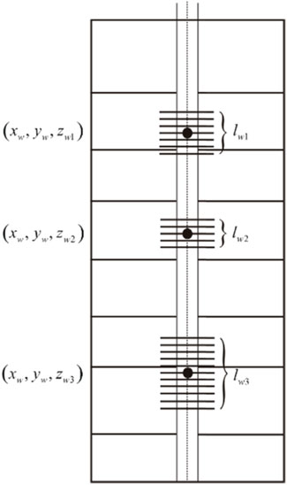
FIGURE 1. Schematic of perforations of a vertical well in multiple layers.
With regard to numerical simulation, in most commercial reservoir simulators, the set of well placement variables are often treated as integers since the simulators require wells to be assigned to discrete grid blocks in the model, namely “connecting gridblocks
The infill well is initially assumed to connect with each layer of the reservoir and then a guess WPI multiplier
Here,
Based on the parameterization method for well placement, the problem considered here can be given as the following formulation:
where
In the hydrocarbon production problems, the objective function can be any user-specified performance measure, such as cumulative oil production or recovery factor and net present value (NPV). This paper considers the negative of the reservoir NPV increment due to infilling wells as the minimization objective function
As for infill project, the outflows of cash include not only the operational costs of existing wells but also the capital expenditures associated with new wells drilled in the reservoir. The capital expenditures consist of the initial investment for drilling new wells and the need for additional surface facilities at the start of the infill project. The operational costs include costs of water treatment and disposal for production wells and water injection for injection wells in each time interval. The incoming cash flow is the profit of oil production from production wells. Thus, the net present value of the infill project can be further defined as the following equation:
where,
In this formulation, the NPV increment objective function depends on the oil production rate
The objective function is minimized using an approximate gradient method, SPSA, which has been used successfully for both well placement and well control optimization as discussed in the Introduction. This section first presents an overview of the general SPSA algorithm and its important properties. Then, based on the general SPSA algorithm, some particular procedures with respect to the problem of well placement optimization are illustrated. The last of this section presents an integrated framework that developed to couple the reservoir simulator with the SPSA algorithm to form an automatic optimization tool for infill well project in oil reservoir.
Assume that noisy measurement
where
The central finite difference method is usually used to approximate the gradient by perturbing the elements of the decision variable vector one at a time and evaluating the objective function for each perturbation, which can be written as
where
It is easy to see that 2p function evaluations are required to approximate the gradient using the finite-difference method, which makes the method increasingly inefficient for application as the problem dimension p grows. The SPSA algorithm provides an efficient alternative by perturbing all vector elements simultaneously to obtain a stochastic gradient approximation
where
The basic step of SPSA algorithm is that: 1) in any given iteration, generate a random perturbation vector
Although the gradient approximation in Eq. 11 requires less function evaluations, it is important to consider the number of iterations required for effective convergence of the algorithm. The SPSA algorithm converges to a local optimum point under some conditions on the SPSA parameters (gain sequences), smoothness of the objective function close to the optimum, and when the properties regarding the perturbation distribution
To satisfy the above conditions, Spall (Gao et al., 2007) provided some useful guidelines to select the perturbation size
where
In its basic form as outlined above, SPSA can only operate on unbounded continuous sets, and is thus unsuited for optimization on our bounded problem. Therefore, in order to enhance the applicability of the SPSA algorithm to solve the problem of well placement optimization, the basic SPSA was modified in this study. Additional treatments include a parameter scaling and constraint handling process, a simple line search procedure and a blocking step.
Firstly, because the well placement and completion optimization formulation is a constrained optimization problem and the elements of optimization variable set
where
In addition, as the gradients are stochastic and approximated, the descent direction might not have sufficient accuracy and the magnitudes of the gradient may change significantly for each new generation. To avoid this problem and guarantee an appropriate step size that minimizes the objective function, we also implement the averaged stochastic gradient as a search direction, i.e.
where each
When the optimization is start, a trial step size
Here,
The optimization algorithm presented above is integrated with the reservoir numerical simulation software Eclipse E100 using Matlab. Figure 2 is the flow chart demonstrating the required steps needed to be taken to run the optimization. For fix number and type of infill wells, well locations are chosen initially using quality map such as reservoir permeability, well productivity, remaining oil, etc. by engineers. Then oil and water flow are calculated using the reservoir flow simulator for the period of the infill program. Total oil and water production and water injection is simulated monthly and imported into Eq. 8 to calculate the net present value for the infill program. This value and the corresponding infill well locations are stored in a data file at each iteration step.

FIGURE 2. Flowchart of the optimization framework.
The next infill well locations are selected by the SPSA algorithm and assigned to new grids in the reservoir. Oil and water production and water injection are again calculated using the flow simulator and another net present value is calculated for new placements. This continuous procedure is an automatic-intelligent approach. The coupling of reservoir simulator and Matlab enables us to repeat this procedure automatically for numerous wells arrangements across the reservoir while the program intelligently produces new allocations.
The integrated framework was first validated with the standard five spot well placements in a synthetic reservoir with lateral homogeneous permeability. Then computationally expensive simulations were performed to attain the best distributions for infill wells intended to enhance development of a mature oil reservoir in China.
To examine the effectiveness of the integrated approach, a multiple-layer reservoir model was constructed on a 25 × 25×4 three-dimensional grid system. The reservoir model parameters used in this simulation are summarized in Table 1. Initial pressures and saturations were calculated by Eclipse’s equilibration facility. The simulation model involves a three-phase oil-water-gas flow without capillary pressure, running for 900 days. The well configuration consists of five wells, four of which are vertical producers with fixed locations at the corners of the reservoir and penetrate the first three layers. The fifth well is a vertical injector and the goal of this example is to find its best location and perforations. Thus, the number of optimization variables is equal to 6, two of which are well location coordinates (I and J) and the others are well production indexes (WPI) in each reservoir layer. The producers are set to maintain a constant liquid production rate of 500STB/day with a lower limit bottom-hole pressure (BHP) of 1 atm, and the injector is controlled using a constant injection rate of 2000 STB/day with a BHP limit of 4500psi.
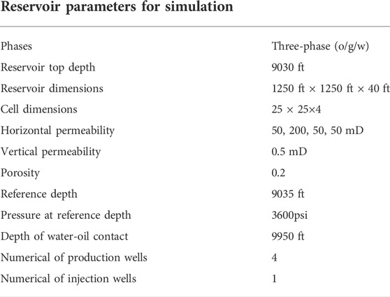
TABLE 1. Reservoir model parameters used in the synthetic model.
The injection well was initially located at grid (5, 5) and was assumed to penetrate each layer fully. Figure 3 represents the corresponding oil saturation distributions in each layer at the end of the simulation. Obviously, the initial guess is not an ideal candidate for the reservoir development. Then, the optimization run was started with a carefully chosen parameter set for SPSA algorithm as discussed above. Table 2 lists parameters used in the SPSA algorithm. We tried several average numbers in SPSA gradient calculation. The values for economic parameters
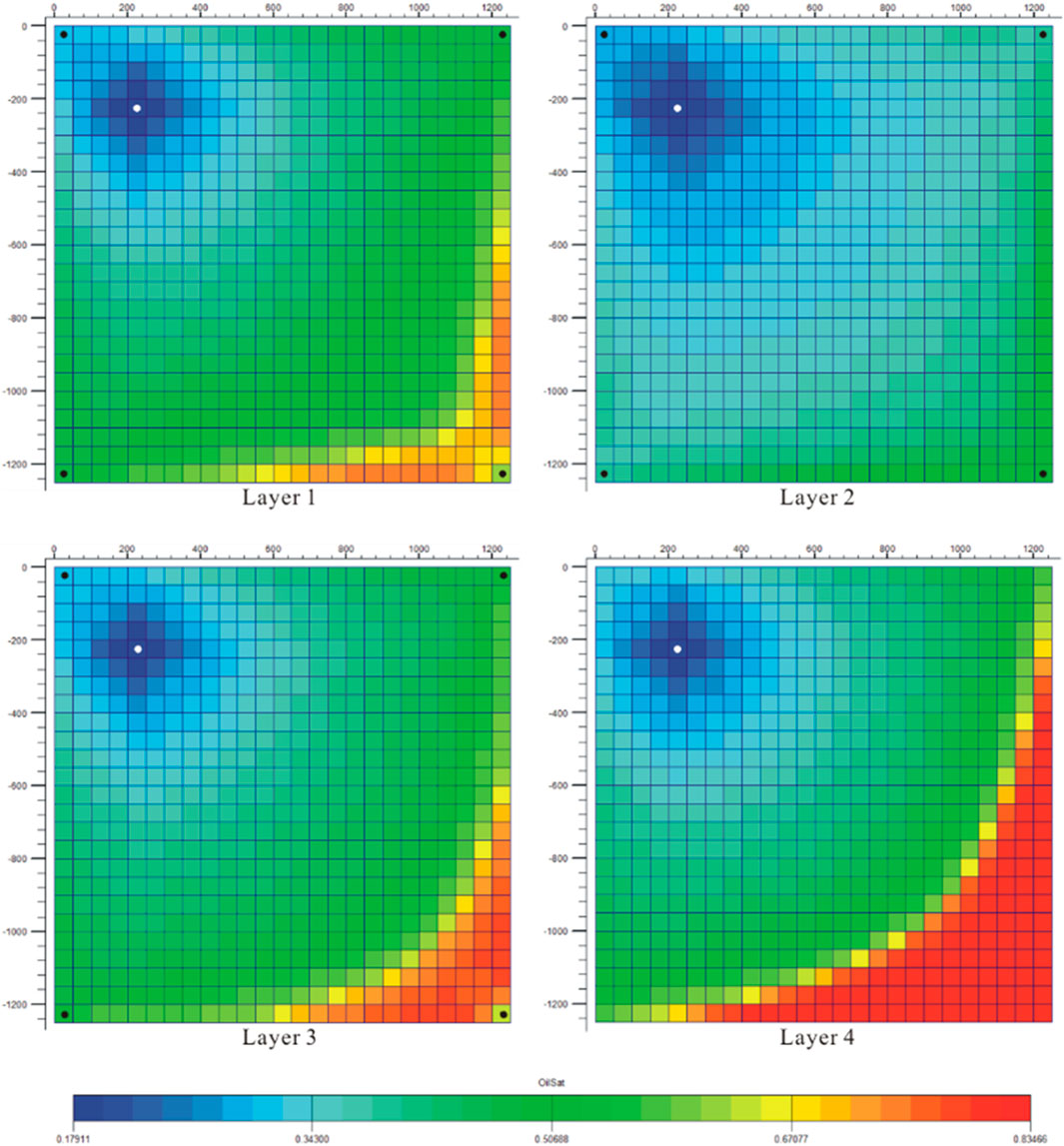
FIGURE 3. Initial well location and the corresponding final oil saturation profiles for the synthetic model.
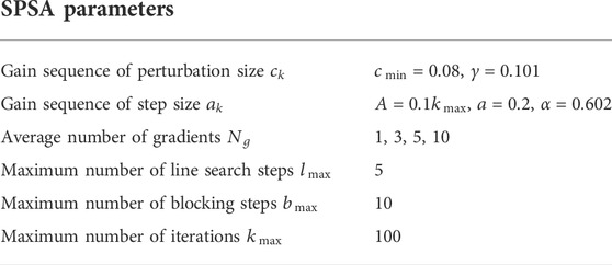
TABLE 2. The applied SPSA options for optimization.
Figure 4 shows the increase in net present value as the SPSA iteration proceeds with different average of the approximate gradients. Note that, in the right part of Figure 4, function evaluations consist of simulation runs for gradient calculation, line search and occasional blocking steps. As can be seen in this figure, within 100 iterations all algorithms converge to a local solution successfully. The algorithm with a single SPSA gradient converges to an NPV of USD 3.927×10⁷ in 86 iterations with approximately 1,000 simulation runs, which is obviously lower than the value obtained from the average SPSA gradient method. Among the three average SPSA methods, the algorithm with average of 10 SPSA gradients took the fewest iterations but the most simulation runs for convergence, while the algorithm with average of 3 SPSA gradients took the most iterations but the fewest simulation runs for convergence. The number of iterations are 64, 51and 41 and the number of simulation runs are 669, 773 and 912, respectively for the cases of
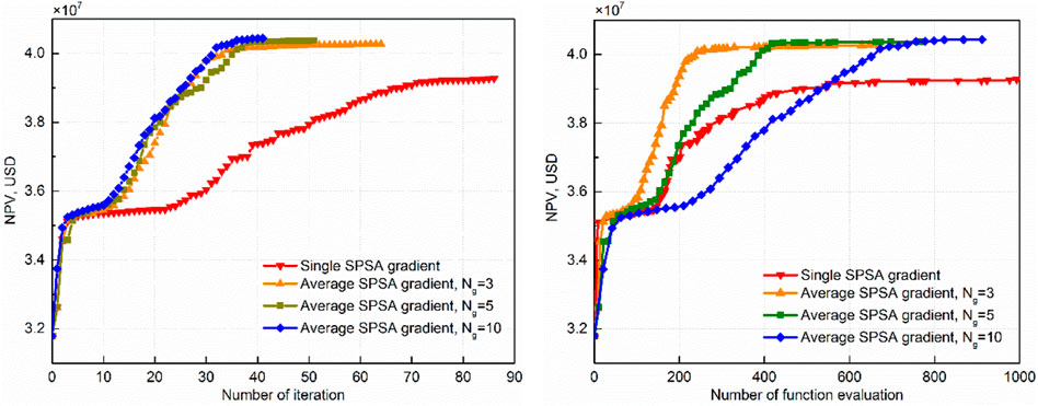
FIGURE 4. Iteration of the objective function for the synthetic model. Left: NPV as a function of iteration number; Right: NPV as a function of objective function evaluation numbers.
The optimal injection well location obtained with the single SPSA method is at grid (17, 13), while the others are all at grid (13, 13). As expected, the injection well is moved toward the center of the rectangle reservoir forming a standard inverted 5-spot pattern by all the optimization algorithms except the single SPSA method. Figure 5 and Figure 6 display the optimum well location that found by the algorithm with average of 10 SPSA gradients on maps of oil saturation distributions at the end of the simulation and the corresponding estimated open fraction of each perforation layer respectively. Note that in the injection well, the second layer is fully shut, while the other three simulation layers is partially open to flow. This is reasonable due to the significantly higher permeability of the second layer than others.
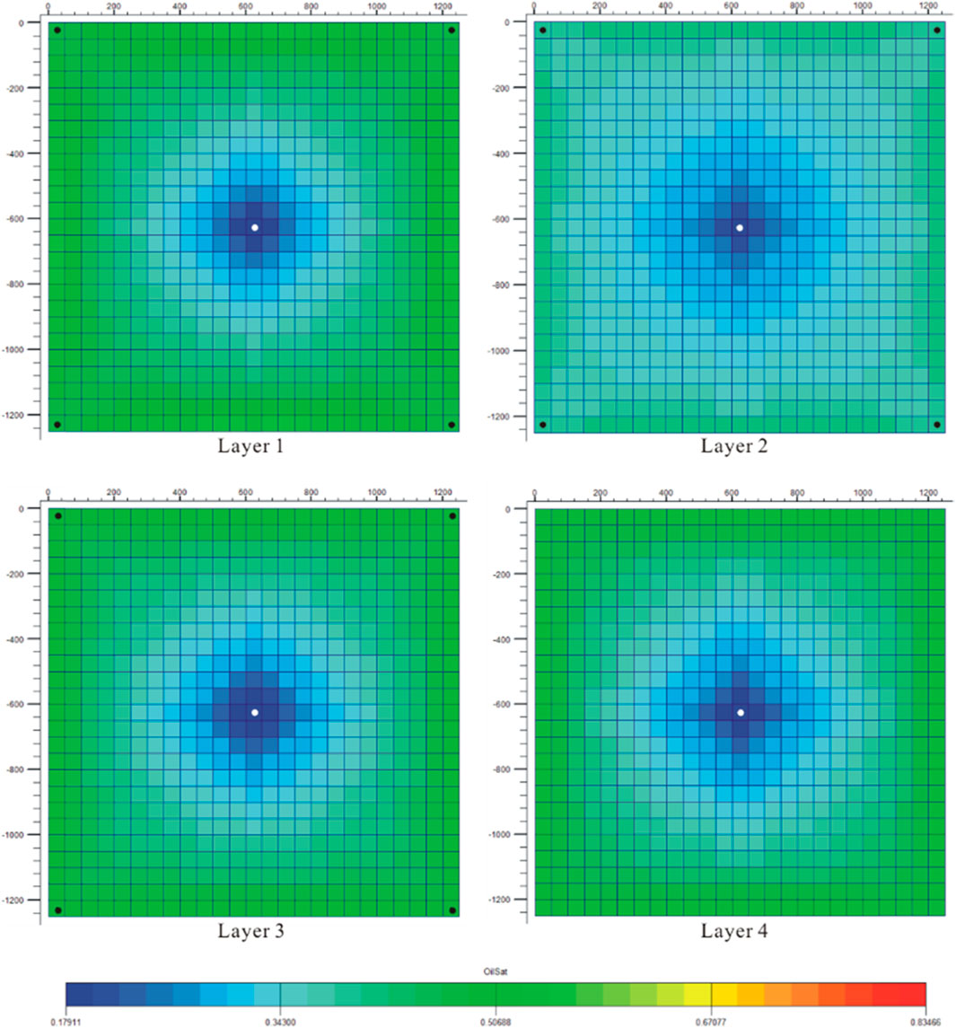
FIGURE 5. Optimized well location and the corresponding final oil saturation profiles for the synthetic model.

FIGURE 6. WPI multiplier for perforations of the injection well for the synthetic model.
It can be confirmed that the presented method is effective for the problem of identifying the optimal well placement or at least the local optimal one. However, the optimization results of the perforation schedule as shown in Figure 6 are more difficult to be verified exactly, because the generalized mix-integer multivariate optimization problem considered in this paper is expected to have very complex objective functions with multiple local solutions and thus the response surface of the objective function with respect to all possible well locations and completions cannot be plotted. For comparison, 10 possible trial well perforation schedules on the optimal well position were tested and the NPV values for the solutions are listed in Table 3.
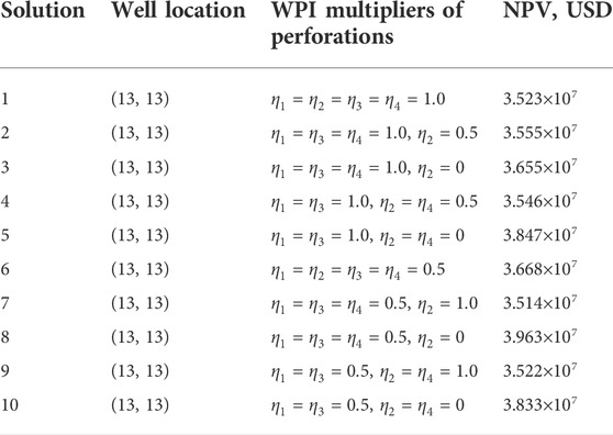
TABLE 3. NPV for some possible well completions.
The highest NPV for all the solutions tried is USD3.963×107 which is slightly lower than the estimated optimum automatically determined with the optimization algorithm. As a remark, we note that the well perforation schedule of solution 8 with the highest NPV is somewhat similar to the estimated: the second layer is shut and the other three layers are partially open to flow for both the two solutions. The results of the numerical experiments confirm the effectiveness of the optimization approach.
The integrated optimization framework was applied to optimize an infilling plan for the mature oil reservoir of Bin8-3 unit in Shengli Oilfield (China). Bin8-3 unit is a lithological reservoir located in Dongying Sag, Bohai Gulf basin, East China, with the Shahejie Formation of the Paleogene being the main petroliferous strata. Primary oil production is from the fourth section of the Shahejie Formation, which is divided into eight layers. The oil bearing area is 345.9acre with an average effective thickness of 91.8 ft. The reservoir has been developed for about 32 years and experienced three stages: Ⅰ. Natural energy drive; Ⅱ. Waterflooding with the basic well patterns (wide spacing inverted seven-spot well pattern); Ⅲ. Waterflooding with the uniformly infilled well patterns (dense spacing inverted seven-spot well pattern). As we can see from Figure 7, the recovery and the water-cut of the reservoir is about 29.5% and 83.1% respectively and the field oil rate continues to decline. A major redevelopment effort to sustain and improve production from this reservoir is selective infill drilling. For an infill plan, the locations and completions of additional wells should be intelligently found to maximize oil production while water production is minimized.
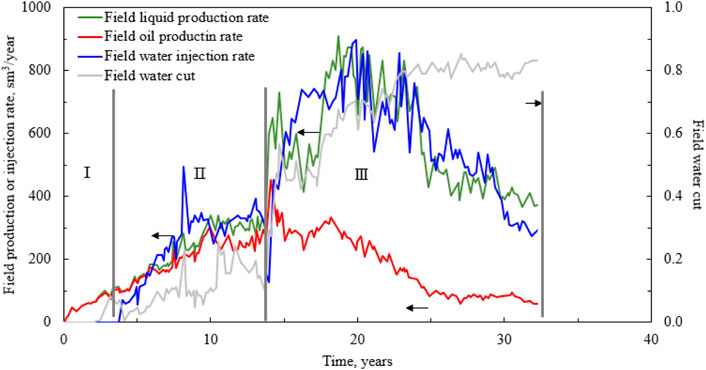
FIGURE 7. Production history curves of Bin8-3 unit in Shengli Oilfield (China).
The reservoir model is constructed from available well log, core analysis and seismic data of the area. There are 55 wells drilled in this reservoir and the wells placement are based on inverted seven-spot pattern. The structure model is made of 85 × 40×8 grid blocks with each cell having uniform planar dimensions of 100 ft × 100 ft but variable vertical dimensions of 2ft–85 ft to reflect the complex geologic structure. The property model (permeability and porosity) is created by using Sequential Gaussian Simulation method and shows extreme heterogeneity both in porosity and permeability distributions. Figure 8 shows the geologic structure of the reservoir and the permeability distribution. Table 4 records the statistical data of the lateral permeability distributions in each layer, including the maximum value, minimum value, average value and median value of each layer. We use variation coefficient, heterogeneity coefficient and max-min ratio of the permeability to characterize the degree of reservoir heterogeneity in each layer, where the three coefficients are defined as follows: variation coefficient is the ratio of the standard deviation of permeability to the mean value in a single layer, i.e.,
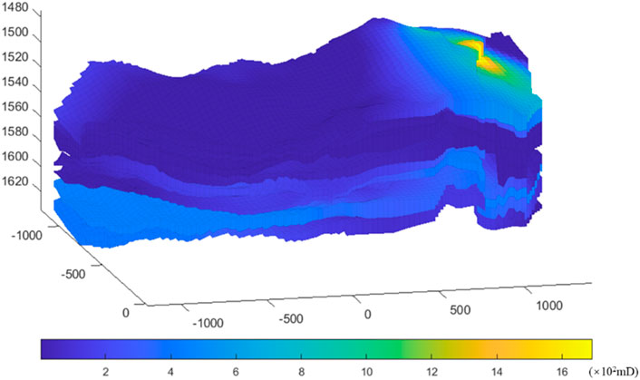
FIGURE 8. Geological structure and permeability field of Bin8-3 unit in Shengli Oilfield (China).
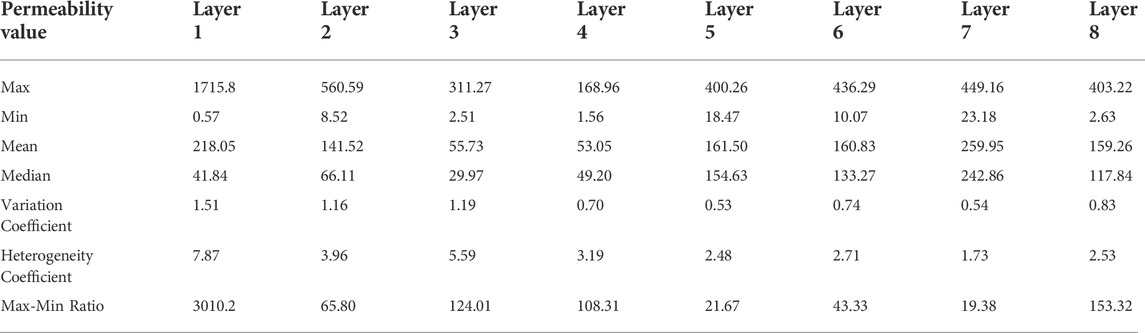
TABLE 4. Characteristics of lateral permeability heterogeneity.
According to the geological research reports of the oilfield, the reservoir lies in a fault-block and has a different oil-water system with the surrounding reservoirs. Thus, we use impermeable boundaries in the numerical model. The model is initialized by the equilibration facility of Eclipse E100. Table 5 lists the basic parameters used for the purpose of simulation. The oil-water and oil-gas relative permeability curves used for oil/water/gas flow simulation are presented in Figure 9A,B respectively.
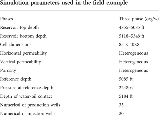
TABLE 5. Reservoir model parameters used in the field example.
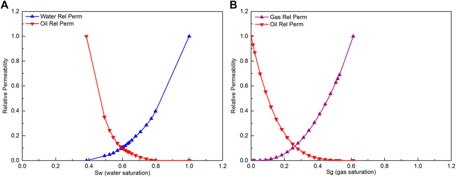
FIGURE 9. Relative permeability curves.
The reservoir model is then calibrated to the historical data available by using an iterative process with a hierarchic structure. In the history matching process, well historical controls are set to be liquid production rate for producers and water injection rate for injectors. The target is to match oil and water production rate of the field (FOPR and FWPR), as well as each producer. We first conduct experimental design to establish reasonable global level uncertainty parameters ranges and inspect their influences on reservoir and production. Then, field liquid production rate (FLPR) is matched to obtain rough estimates of global level pore volume and transmissibility ranges. After the field liquid matching is achieved, we adjust saturation profile to match FOPR and FWPR. While maintaining FOPR and FWPR, we move forward to the well level to improve pore volume and transmissibility ranges. We end the process when acceptable matching results are obtained in both global level and well level. Figure 10 shows a part of the validation results, on which the observation data are represented with circles and the prediction data are represented with curves. From Figure 10, one observes that both oil production (A) and water production (B) match closely with historical data. We use the calibrated numerical model to perform well placement optimization.
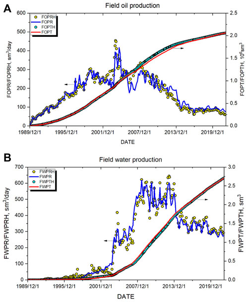
FIGURE 10. Field production history matching results.
To identify the initial locations of infill wells, we first examined the potential regions of poorly swept and poorly drained oil in the reservoir. Figure 11 is the final distribution of remaining oil pore volume after approximate 32 years’ production, which is generated by adding layer upon layer. It is observed that there are amount remaining oil scattered in the eastern part of the reservoir, mainly near the faults and the boundary of the reservoir. In order to boost oil production rate, we tried to place four new vertical production wells in the oil-rich regions and located them initially at the points marked with white circles in Figure 11. Then, the proposed optimization framework was used to find the optimal placements of the four new wells, including the locations and their completions in such a complex multi-layer reservoir. To get a more reliable solution, three cases of optimization work were carried out. In case 1, the well locations are fixed at the initial guess and only completions are optimized. This case with the initial configuration of the infill wells is used as the reference case because of the assumed potential oil productivity in the selected oil-rich regions. In case 2, the well location and the well completion are optimized simultaneously with the SPSA algorithm and we refer to it as simultaneous joint optimization problem. In case 3, the joint optimization problem is broken into two steps and we refer to it as sequential joint optimization framework. In the first step, the optimal well location problem is solved with the SPSA algorithm with the well penetrating all layers fully. After the optimal location of the wells is estimated, we perform the completion optimization step, in which, the well locations are fixed and specified and the completions of each well are optimized.
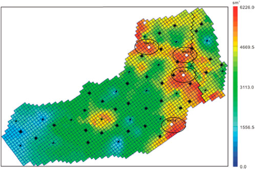
FIGURE 11. Initial locations of infill wells on map of remaining oil distribution at the end of production history.
To compare the results of the three cases, we performed the optimization runs with the same initial conditions. Besides, a simulation run without infill wells was also conducted for comparison. All infill wells are initially assumed to penetrate each layer fully and maintain a constant liquid production rate of 95STB/day with a lower limit bottom-hole pressure of 1 atm. The existing wells are set to continue to work in their last control mode. The duration of the infill project is set to 10 years. Algorithm with average of 5 SPSA gradients is used. The maximum allowed iteration times of the optimization algorithm is 500 and the optimization run is terminated ahead after it encountered 10 times of continuous trials of ineffectual iteration. Other parameters that related to the optimization are the same with the example of the synthetic model. The NPV value for the simulation run without infill wells is USD2.111×107 and the values for the optimization runs are shown in Figure 12. Results show that, even without optimization, the economic revenue of the infill project significantly surpasses the case of no infill wells. Optimization of infill well location and completions enhances the performance of the infill project. In case 1, the optimization converged after 311 algorithm iterations, and NPV increased from USD5.845×107 at the initial guess to USD6.992×107 at convergence. In case 2, the optimization converged after 39 algorithm iterations, and NPV increased to USD7.266×107 at convergence. In case 3, the optimization converged after 407 algorithm iterations which include 21 iterations for well location optimization and 386 iterations for well completion optimization, and NPV increased to USD8.577×107 at convergence. Comparing the NPV values for the optimization runs corresponding to case 2 and case 3 with the optimization run for case 1 shows that the optimization runs for well locations, regardless of the order of optimizing well completions, obtained higher NPV values than the optimization run for well completions only. Thus, it can be inferred that for the subject reservoir, NPV is more sensitive to the well location than to the completions of the wells.
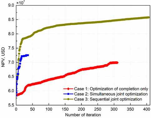
FIGURE 12. Objective function value versus number of iterations for three optimization cases in the field application.
It is also important to mention that in the case of simultaneous joint optimization (case 2), the algorithm iteration was stopped by the convergence criterion of allowance maximum number of blocking steps before it arrived at a real optimal solution. This can be justified by Figure 13, in which the optimization was continued with regard to well completions based on the obtained optimal well locations and as a result the NPV value increased from USD7.266 × 107 to USD7.872 × 107 after extra 205 algorithm iterations. The main reason that SPSA does not find the optimal well completions in case 2 is that the algorithm proceeded first to a solution with optimal well locations which is similar with the first plateau observed in the validation example, and in the following iterations, the increase of NPV value caused by perturbation of well completion parameters was offset by the decrease of NPV value caused by perturbation of well location parameters due to the natural property of simultaneous perturbation of SPSA algorithm. Based on these results, it is not unreasonable to recommend the sequential joint optimization, when using SPSA as the algorithm, as the optimization framework for obtaining the best scheme for the placement of infill wells.
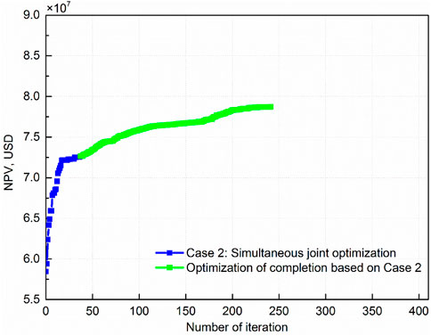
FIGURE 13. Objective function value versus number of iterations for continued optimization of completion based on Case 2.
As mentioned above, the convergence of the three cases requires 311, 39, 407 iterations respectively, and one iteration requires running 10 times of the model, and the time of running 1 time of the model is about 66 s. Therefore, in the current computer configuration, the convergence of the three cases take 57 h, 7.15 h, and 74.62 h, respectively.
Initial and final locations of the infill production wells for case 2 and case 3 are shown in Figure 14, where crosses represent for the results of Case 2 and pentagrams for the results of Case 3, respectively. The final WPI multipliers for perforations at the four infill wells are shown in Figure 15 for case 2 and Figure 16 for case 3, respectively. Since the initial locations of the infill wells are all in the oil-rich regions, we expect an optimum solution that has less adjustments with respect to the initial guess. However, our algorithm did not achieve this for all infill wells. For example, Well 1 is moved far away from its initial location to another oil-rich region both in case 2 and in case 3, and Well 3 is moved toward a margin region that is not controlled by the original well patterns in case 3. Although significant changes in the location of these wells occurred, a general trend can be observed that the infill production wells are moved far away from the injection wells to somewhere nearby the boundary of the reservoir or the faults where a considerable amount of oil remains. By contrast, changes in the completions of the wells are specialized and very dependent on the well location. Comparing the WPI multipliers of the four infill wells in case 2 shows that the best obtained completions of these wells are significantly different with each other because of the different obtained well locations for these four wells. The same result can be observed in case 3. However, comparing the best obtained completion of well 2 in case 2 and case 3 shows that very similar well completions are obtained because of the same well locations for these two cases.

FIGURE 14. Optimal locations of infill wells on the map of remaining oil distribution for two optimization cases in the field application.
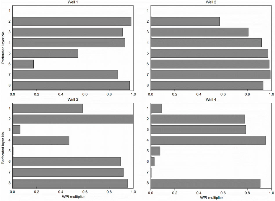
FIGURE 15. WPI multipliers for perforations of the four infill wells, Case 2.
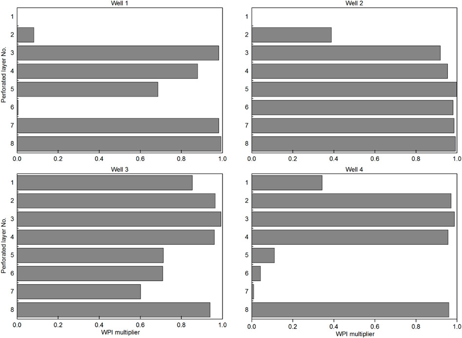
FIGURE 16. WPI multipliers for perforations of the four infill wells, Case 3.
Optimizing quality location and completions in the mature reservoir for infill well placement is a very complex function of various factors including reservoir properties such as permeability, porosity, net thickness and reservoir structure etc., well configuration and production control of existing producers and injectors, distribution of remaining oil and economic indexes. Undoubtedly, it is hard to set up a universally applicable principle to guard the well placement of infill wells. Although in practice locations and completions can be proposed by experienced reservoir engineers, the considerable difference between infill project revenues obtained by using optimization method and by selecting based on best engineering practice makes well placement across the reservoir a crucial practice and magnifies the need for employing the integrated framework to design infill well locations intelligently.
In this study, an integrated framework is developed to couple the reservoir flow simulator and a SPSA algorithm based optimizer to find optimal infill well locations and completions for enhancing waterflooding recovery of a mature oil reservoir. A synthetic reservoir model with four production wells located in the corners is created to validate the effectiveness of the integrated approach. The integrated framework is used to find the best obtained injection well location and also the completion in the reservoir. A complex heterogeneous reservoir model is then constructed by using the data of a mature oil reservoir in Shengli Oilfield in China to design an optimal 10 years infill drilling program. According to the remaining oil distributions, four new producers are placed in the oil-rich regions as the start of the optimizations. Since the potential regions are assumed to be the best candidates of infill wells, both only well completions optimization with the fixed initial locations and coupled well locations and completions optimization are performed by the integrated framework and the results are compared. The main conclusions of this study are as follows:
1) The well placement problem given here consists of joint optimization of the location and completion of a vertical well. Well location is parameterized in terms of discrete integral lattice variables and well completion is represented by WPI multiplier for the connection with each simulation layer. With this parameterization, the well placement problem is simplified and a variant of SPSA algorithm can be applied to obtain optimal well placement which is easy to implement and computationally feasible.
2) The algorithm with average SPSA gradients obtains better results than does the single SPSA gradient method. Although it needs more function evaluations to obtain the approximate gradients for a single recursion step, the algorithm with average SPSA gradients converges more quickly than the single SPSA gradient method.
3) The proposed framework is successfully applied for the optimization of infill well location and completion in a mature oilfield with high water-cut and heterogeneous reservoir properties. For the complex reservoir, the sequential optimization shows superior performance than the simultaneous optimization for jointly optimizing well location and well completion.
4) In joint optimization of well location and completion, the convergence for optimal well completion is significantly slower than for the optimal well location. Moreover, the NPV value is more sensitive to well location than to well completion parameters for extremely heterogeneous reservoir.
This work provides an initial attempt to formulate and solve a development optimization problem by focusing on well location and completion optimizations that frequently encountered in the redevelopment of mature oilfields. The more generalized problem may also involve the type and the number of infill wells, drilling schedule, production controls, and the reservoir life cycle. However, considering all of these decision variables while trying to maximize oil recovery in a real reservoir, turns into a complex optimization problem which is not only hard to describe in mathematical formulas but also hard to solve in an efficient way. On the other hand, it has been widely recognized that optimization by fixing some of the decision variables a priori must lead to the problem of suboptimality. Thus, more sophisticated treatment approaches and solution algorithms are required to tackle the complex problem. Besides, as any description of realistic objects, there is a large degree of uncertainty in describing the physical properties of the subsurface reservoirs which makes the problem further complicated. Geologic uncertainty should be considered to reduce the risk of an infill plan. In future work, we will first extend our approach to well placement optimization of more complicated wells, such as horizontal wells and multilateral wells. Then, we will try to combine well placement and control optimizations under geologic uncertainty to solve a more generalized problem. In addition, several other optimization algorithms may be compared in solving our problems.
The original contributions presented in the study are included in the article/Supplementary Material, further inquiries can be directed to the corresponding author.
CL: writing calculation programs, analyzing data and writing the paper. CF: Establishing the reservoir numerical simulation model YH: Model verification HZ: correcting language errors ZZ: Debug code SW: guiding the first author to write calculation programs and paper.
This work is supported by the National Science and Technology Major Project (Project No. 2017ZX05009005-004).
The authors would express their appreciation to the Project for contribution of research fund. Authors would also like to acknowledge reviewers for their constructive comments and careful revision of this paper.
CF is employed by CNPC Logging Company Limited Geological Research Institute.
YH and HZ are employed by CNPC Exploration and Development Research Institute of Changqing Oilfield Branch.
The remaining authors declare that the research was conducted in the absence of any commercial or financial relationships that could be construed as a potential conflict of interest.
All claims expressed in this article are solely those of the authors and do not necessarily represent those of their affiliated organizations, or those of the publisher, the editors and the reviewers. Any product that may be evaluated in this article, or claim that may be made by its manufacturer, is not guaranteed or endorsed by the publisher.
Algorithm 1. Modified SPSA algorithm for well placement optimization
Modified SPSA Algorithm.
Set iteration number
Initialize the optimization variable
While
Update
while
Cut gain step using
end
if
Accept the kthth iteration step;
end
if
Reject the kthth iteration step; Try a new set of
end
end.
Afshari, S., Aminshahidy, B., and Pishvaie, M. R. (2015). Well placement optimization using differential evolution algorithm. Iran. J. Chem. Chem. Eng. (IJCCE) 34 (2), 109–116.
Afshari, S., Pishvaie, M. R., and Aminshahidy, B. (2014). Well placement optimization using a particle swarm optimization algorithm, a novel approach. Petroleum Sci. Technol. 32 (2), 170–179. doi:10.1080/10916466.2011.585363
Awotunde, A. A. (2016). Generalized field-development optimization with well-control zonation. Comput. Geosci. 20 (1), 213–230. doi:10.1007/s10596-016-9559-2
Badru, O. (2003). Well-placement optimization using the quality map approach. Stanford University. MS. Thesis.
Bangerth, W., Klie, H., Wheeler, M. F., Stoffa, P. L., and Sen, M. K. (2006). On optimization algorithms for the reservoir oil well placement problem. Comput. Geosci. 10 (3), 303–319. doi:10.1007/s10596-006-9025-7
Beckner, B. L., and Song, X. (1995). “Field development planning using simulated annealing-optimal economic well scheduling and placement,” in SPE annual technical conference and exhibition, held in Dallas, U.S.A., October, 1995 (Dallas, TX: Society of Petroleum Engineers), 22–25.
Bellout, M. C., Echeverría Ciaurri, D., Durlofsky, L. J., Foss, B., and Kleppe, J. (2012). Joint optimization of oil well placement and controls. Comput. Geosci. 16, 1061–1079. doi:10.1007/s10596-012-9303-5
Bouzarkouna, Z., Ding, D. Y., and Auger, A. (2013). Partially separated metamodels with evolution strategies for well-placement optimization. SPE J. 18 (6), 1003–1011. doi:10.2118/143292-pa
Bouzarkouna, Z., Ding, D. Y., and Auger, A. (2012). Well placement optimization with the covariance matrix adaptation evolution strategy and meta-models. Comput. Geosci. 16 (1), 75–92. doi:10.1007/s10596-011-9254-2
Chang, Y., Petvipusit, K. R., and Devegowda, D. (2015). “Multi-objective optimization coupled with dimension-wise polynomial-based approach in smart well placement under model uncertainty,” in SPE reservoir simulation symposium (Houston, Texas, USA, February 2015 OnePetro). SPE-173291-MS
da Cruz, P. S., Horne, R. N., and Deutsch, C. V. (2004). The quality map: A tool for reservoir uncertainty quantification and decision making. SPE Reserv. Eval. Eng. 7 (1), 6–14. doi:10.2118/87642-pa
Do, S. T., Forouzanfar, F., and Reynolds, A. C. (2012). Estimation of optimal well controls using the augmented Lagrangian function with approximate derivatives. IFAC Proc. Vol. 45 (8), 1–6. doi:10.3182/20120531-2-no-4020.00021
Do, S. T., and Reynolds, A. C. (2013). Theoretical connections between optimization algorithms based on an approximate gradient. Comput. Geosci. 17 (6), 959–973. doi:10.1007/s10596-013-9368-9
Emerick, A. A., Silva, E., Messer, B., Almeida, L. F., Dilza, S., Pacheco, M. A. C., et al. (2009). “Well placement optimization using a genetic algorithm with nonlinear constraints,” in SPE reservoir simulation symposium The Woodlands, Texas February 2009 (Society of Petroleum Engineers). doi:10.2118/118808-MS
Forouzanfar, F., Poquioma, W. E., and Reynolds, A. C. (2016). Simultaneous and sequential estimation of optimal placement and controls of wells with a covariance matrix adaptation algorithm. SPE J. 21 (2), 501–521. doi:10.2118/173256-pa
Forouzanfar, F., and Reynolds, A. C. (2014). Joint optimization of number of wells, well locations and controls using a gradient-based algorithm. Chem. Eng. Res. Des. 92 (7), 1315–1328. doi:10.1016/j.cherd.2013.11.006
Forouzanfar, F., Reynolds, A. C., and Li, G. (2012). Optimization of the well locations and completions for vertical and horizontal wells using a derivative-free optimization algorithm. J. Petroleum Sci. Eng. 86, 272–288. doi:10.1016/j.petrol.2012.03.014
Forouzanfar, F., and Reynolds, A. C. (2013). Well-placement optimization using a derivative-free method. J. Petroleum Sci. Eng. 109, 96–116. doi:10.1016/j.petrol.2013.07.009
Gao, G., Li, G., and Reynolds, A. C. (2007). A stochastic optimization algorithm for automatic history matching. SPE J. 12 (2), 196–208. doi:10.2118/90065-pa
Guimaraes, M. S., Schiozer, D. J., and Maschio, C. (2005). “Use of streamlines and quality map in the optimization of production strategy of mature oil fields,” in SPE Latin American and Caribbean Petroleum Engineering Conference, Rio de Janeiro, Brazil, June, 2005 (Society of Petroleum Engineers). doi:10.2118/94746-MS
Han, D. K. (2010). On concepts, strategies and techniques to the secondary development of China's high water-cut oilfields. Petroleum Explor. Dev. 37 (5), 583–591. doi:10.1016/s1876-3804(10)60055-9
Han, D. K. (2007). Precisely predicting abundant remaining oil and improving the secondary recovery of mature oilfields. Acta Pet. Sin. 28 (2), 73–78.
Isebor, O. J., Durlofsky, L. J., and Ciaurri, D. E. (2014). A derivative-free methodology with local and global search for the constrained joint optimization of well locations and controls. Comput. Geosci. 18, 463–482. doi:10.1007/s10596-013-9383-x
Isebor, O. J., Echeverría Ciaurri, D., and Durlofsky, L. J. (2014). Generalized field-development optimization with derivative-free procedures. SPE J. 19 (5), 891–908. doi:10.2118/163631-pa
Jesmani, M., Bellout, M. C., Hanea, R., and Foss, B. (2016). Well placement optimization subject to realistic field development constraints. Comput. Geosci. 20 (6), 1185–1209. doi:10.1007/s10596-016-9584-1
Jesmani, M., Jafarpour, B., Bellout, M. C., and Hanea, R. G. (2016). “Application of simultaneous perturbation stochastic approximation to well placement optimization under uncertainty,” in ECMOR XV-15th European Conference on the Mathematics of Oil Recovery.
Kharghoria, A., Cakici, M., and Narayanasamy, R. (2003). “Productivity-based method for selection of reservoir drilling target and steering strategy,” in SPE/IADC Middle East Drilling Technology Conference and Exhibition, Abu Dhabi, United Arab Emirates, October, 2003 (Abu Dhabi: United Arab Emirates Society of Petroleum Engineers). doi:10.2118/85341-MS
Li, G., and Reynolds, A. C. (2011). Uncertainty quantification of reservoir performance predictions using a stochastic optimization algorithm. Comput. Geosci. 15 (3), 451–462. doi:10.1007/s10596-010-9214-2
Li, L., and Jafarpour, B. (2012). A variable-control well placement optimization for improved reservoir development. Comput. Geosci. 16, 871–889. doi:10.1007/s10596-012-9292-4
Li, L., Jafarpour, B., and Mohammad-Khaninezhad, M. R. (2013). A simultaneous perturbation stochastic approximation algorithm for coupled well placement and control optimization under geologic uncertainty. Comput. Geosci. 17, 167–188. doi:10.1007/s10596-012-9323-1
Montes, G., Bartolome, P., and Udias, A. L. (2001). “The use of genetic algorithms in well placement optimization,” in SPE Latin American and Caribbean Petroleum Engineering Conference, Buenos Aires, Argentina, March 2001 (Buenos Aires, Argentina: Society of Petroleum Engineers). doi:10.2118/69439-MS
Nwankwor, E., Nagar, A. K., and Reid, D. C. (2013). Hybrid differential evolution and particle swarm optimization for optimal well placement. Comput. Geosci. 17, 249–268. doi:10.1007/s10596-012-9328-9
Onwunalu, J. E., and Durlofsky, L. J. (2010). Application of a particle swarm optimization algorithm for determining optimum well location and type. Comput. Geosci. 14 (1), 183–198. doi:10.1007/s10596-009-9142-1
Ozdogan, U., and Horne, R. N. (2006). Optimization of well placement under time-dependent uncertainty. SPE Reserv. Eval. Eng. 9 (2), 135–145. doi:10.2118/90091-pa
Pouladi, B., Karkevandi-Talkhooncheh, A., Sharifi, M., Gerami, S., Nourmohammad, A., and Vahidi, A. (2020). Enhancement of SPSA algorithm performance using reservoir quality maps: Application to coupled well placement and control optimization problems. J. Petroleum Sci. Eng. 189, 106984. doi:10.1016/j.petrol.2020.106984
Salmachi, A., Sayyafzadeh, M., and Haghighi, M. (2013). Infill well placement optimization in coal bed methane reservoirs using genetic algorithm. Fuel 111, 248–258. doi:10.1016/j.fuel.2013.04.022
Sarma, P., and Chen, W. H. (2008). “Efficient well placement optimization with gradient-based algorithms and adjoint models,” in Intelligent Energy Conference and Exhibition , Amsterdam, The Netherlands, February 2008 (Amsterdam, Netherlands: Society of Petroleum Engineers). doi:10.2118/112257-MS
Spall, J. C. (2000). Adaptive stochastic approximation by the simultaneous perturbation method. IEEE Trans. Autom. Contr. 45 (10), 1839–1853. doi:10.1109/tac.2000.880982
Spall, J. C. (1994). “Developments in stochastic optimization algorithms with gradient approximations based on function measurements,” in Proceedings of the 26th conference on Winter simulation, held in Lake Buena Vista, FL, USA (Society for Computer Simulation International), 207–214. doi:10.1109/WSC.1994.717126
Spall, J. C. (1998). Implementation of the simultaneous perturbation algorithm for stochastic optimization. IEEE Trans. Aerosp. Electron. Syst. 34 (3), 817–823. doi:10.1109/7.705889
Spall, J. C. (1992). Multivariate stochastic approximation using a simultaneous perturbation gradient approximation. IEEE Trans. Autom. Contr. 37 (3), 332–341. doi:10.1109/9.119632
Taware, S. V., Park, H., Datta-Gupta, A., Shyamal, B., Tomar, A. K., and Rao, H. S. (2012). “Well placement optimization in a mature carbonate waterflood using streamline-based quality maps,” in SPE Oil and Gas India Conference and Exhibition, Mumbai, India, March, 2012 (Society of Petroleum Engineers). doi:10.2118/155055-MS
Temizel, C., Zhiyenkulov, M., Ussenova, K., and Tilek, K. (2018). “Optimization of well placement in waterfloods with optimal control theory under geological uncertainty,” in SPE Annual Technical Conference and Exhibition, Dallas, Texas, USA, September, 2018 (OnePetro). doi:10.2118/191660-MS
Vlemmix, S., Joosten, G. J. P., Brouwer, R., and Jansen, J. D. (2009). “Adjoint-based well trajectory optimization,” in EUROPEC/EAGE Conference and Exhibition, Amsterdam, The Netherlands, June, 2009 (Society of Petroleum Engineers). doi:10.2118/121891-MS
Wang, C., Li, G., and Reynolds, A. C. (2007). Optimal well placement for production optimization Eastern Regional Meeting. Lexington, Kentucky, USA, October 2007: Society of Petroleum Engineers.
Wang, C., Li, G., and Reynolds, A. C. (2009). Production optimization in closed-loop reservoir management. SPE J. 14 (3), 506–523. doi:10.2118/109805-pa
Yeten, B., Durlofsky, L. J., and Aziz, K. (2003). Optimization of nonconventional well type, location, and trajectory. SPE J. 8 (3), 200–210. doi:10.2118/86880-pa
Keywords: mature oilfields, secondary development, infill wells, well placement optimization, simultaneous perturbation stochastic approximation (SPSA)
Citation: Li C, Fang C, Huang Y, Zuo H, Zhang Z and Wang S (2022) Infill well placement optimization for secondary development of waterflooding oilfields with SPSA algorithm. Front. Energy Res. 10:1005749. doi: 10.3389/fenrg.2022.1005749
Received: 28 July 2022; Accepted: 27 October 2022;
Published: 16 November 2022.
Edited by:
Luis Puigjaner, Universitat Politecnica de Catalunya, SpainReviewed by:
Bicheng Yan, King Abdullah University of Science and Technology, Saudi ArabiaCopyright © 2022 Li, Fang, Huang, Zuo, Zhang and Wang. This is an open-access article distributed under the terms of the Creative Commons Attribution License (CC BY). The use, distribution or reproduction in other forums is permitted, provided the original author(s) and the copyright owner(s) are credited and that the original publication in this journal is cited, in accordance with accepted academic practice. No use, distribution or reproduction is permitted which does not comply with these terms.
*Correspondence: Shuoliang Wang, d2FuZ3NodW9saWFuZ0BjdWdiLmVkdS5jbg==
Disclaimer: All claims expressed in this article are solely those of the authors and do not necessarily represent those of their affiliated organizations, or those of the publisher, the editors and the reviewers. Any product that may be evaluated in this article or claim that may be made by its manufacturer is not guaranteed or endorsed by the publisher.
Research integrity at Frontiers
Learn more about the work of our research integrity team to safeguard the quality of each article we publish.