An Optimization-Based Method for the Explicit Production Data Analysis of Gas Wells

This work aims at the exploration of production data analysis (PDA) methods without iterations. It can overcome limitations of the advanced type curve analysis relying on the iterative calculation of material-balance pseudotime and current explicit methods reckoning on specific production schedule assumptions. The dynamic material balance equation (DMBE) is strictly proved by the integral variable substitution based on the gas flow equation under the boundary dominated flow (BDF) condition and the static material balance equation (SMBE) of a gas reservoir. We introduce the pseudopressure level function γ(p) and the recovery factor function R(p) to rewrite the DMBE in terms of observed variable Y and estimated variable Y_e; then the PDA can be transformed into an optimization problem of minimizing the error between Y and Y_e. An optimization-based method for the explicit production data analysis of gas wells (OBM-EPDA), therefore, is developed in the paper, capable of determining the BDF constant and gas reserves explicitly and accurately for variable rate and/or variable flowing pressure systems. Three stimulated cases demonstrate the applicability and validity of OBM-EPDA with small errors less than 1% for estimated values of both reserves and Y. Not second to previous studies, the field case analysis further proves its practicability. It is shown that the nonlinear relation of γ to R can be represented by a polynomial function merely dependent on the inherent properties of the gas production system even before sorting out the production data. The errors of observed variable Y provided by OBM-EPDA facilitate the data quality control, and the elimination of outliers not subject to the BDF condition improves the reliability of the analysis. For various gas systems producing whether at a constant rate, a constant bottomhole pressure (BHP), or under variable rate and variable BHP conditions, the proposed method gives insights into the well-controlled volume and production capacity of the gas well whether in a low-pressure or high-pressure gas reservoir, where the compressibilities of rock and bound water are considered.

Introduction

Reservoir engineers often rely on well testing (Chaudhry, 2003; Kamal, 2009; Spivey and Lee, 2013) to estimate parameters such as permeability, skin and average reservoir pressure, and use the measured static pressure data combined with the material balance equation (Moghadam et al., 2009; Moghadam et al., 2011; Ahmed and Meehan, 2012) to determine gas reserves. These means that entail well shut-ins or tests to obtain formation or gas well information, however, have been subject to the high cost. The past few decades have witnessed the development of low-cost production data analysis (PDA) methods (Mattar and Anderson, 2003; Sun, 2015; Behmanesh et al., 2018). PDA of gas wells refers to the utilization of daily recorded production data such as production, bottomhole pressure (BHP) and cumulative gas production to interpret the attributes of gas wells or gas reservoirs by an empirical or analytical model. It can determine the vital parameters such as well-controlled reserves and deliverability, even permeability, skin factor and other useful parameters at a low cost which could powerfully support the performance analysis and efficient development of gas reservoirs.

The research on PDA can be traced back to the production decline laws presented by Arps (1945). These empirical models are based on statistics, and the applicability to constant-BHP production systems was not proved rigorously at that time.

Combining Arps’ decline curves with the analytical solution of the constant-pressure case, Fetkovich (1980), Fetkovich et al. (1987) proposed the idea of using type curve fitting to analyze the changes in production rate. He proved that the production rate vs. time relationship under the constant BHP condition for liquid production systems satisfies the exponential decline law during the late BDF, which overcomes the empiricism of Arps’ curves.

Carter (1981), Carter (1985) introduced the variable λ [ = μ_iC_gi/(μC_g)] to explain the changes in gas viscosity and compressibility, so as to analyze the rate vs. time data of constant-BHP gas wells. The drawdown parameter λ in Carter’s curves represents the average value from bottomhole pressure p_wf to original formation pressure p_i, which does not vary with the decreasing reservoir pressure. Thus, it is only an approximate method for analyzing the constant-BHP data of gas wells.

Blasingame and Lee (1988) developed an iteration method for PDA based on the previous BDF liquid solution (Blasingame and Lee, 1986), termed “variable-rate reservoir limits testing of gas wells,” by introducing the material balance pseudotime and pseudopressure functions. This approach entails the iterations on average reservoir pressure, material balance pseudotime, BDF slope (m_bdf) and BDF constant (b) on the basis of the transformation of pseudovariables and the static material balance equation (SMBE) of constant-volume gas reservoirs, where variations of production schedule and change in gas properties are considered. Its theory has gradually become the basis of many following PDA methods. The introduction of material balance pseudotime function makes it possible to analyze variable-rate data, but its iterative calculation also seems unavoidable on account of the implied average reservoir pressure.

Blasingame et al. (1991) proposed a method for PDA of variable pressure drop/variable flowrate systems using constant BHP solution, which depends on the conversion between the constant pressure analog time function and the constant rate function. For gas wells, however, the analysis still involves the implementation of the iterative process of Blasingame and Lee (1988) to determine the BDF slope m_bdf and the BDF constant b.

Palacio and Blasingame (1993) proposed a type-curve analysis method for gas well production data (Agarwal et al., 1998; Agarwal et al., 1999) based on the gas flow equation during BDF (Blasingame and Lee, 1988). It is proved that the relation between decline curve dimensionless rate q_dD and dimensionless time t_dD defined by the pseudopressure and the material balance pseudotime follows the harmonic decline law in the BDF stage. Blasingame’s type curve is a representative of modern rate transient analysis (RTA) methods. In addition, other type-curve analysis methods such as Agarwal-Gardner curve (Agarwal et al., 1998; Agarwal et al., 1999) and normalized pressure integral (NPI) (Blasingame et al., 1989) have the similar analysis procedure, but the plot functions are different.

Canard (1994) and Callard and Schenewerk (1995) applied the diagnostic type-curve, which incorporates the instantaneous BHP to both the production rate and the cumulative production for PDA. The concept of viscosity-compressibility normalized cumulative was proposed for the first time, and the production data of gas wells can be analyzed by using the slightly compressible liquid solution through pseudopressure and viscosity-compressibility normalization.

Mattar and McNeil (1995), Mattar and McNeil (1998) pointed out that the ratio of pressure to Z-factor (p/Z) at BHP can be used to replace the p/Z value at the average formation pressure to perform the material balance analysis of constant-volume gas reservoirs, and presented the flowing material balance procedure for the estimation of gas in place. In fact, the slope of the linear relationship between p/Z and cumulative gas production G_p under the BHP condition, however, is not equal to the result under the average reservoir pressure condition. Therefore, this method has certain theoretical defects and may not be suitable for gas wells with variable rate or strong compressibility effects.

Ansah et al. (1996), Ansah et al. (2000) correlated the gas viscosity-compressibility product μ⋅C_g with p/Z, and used first-order polynomial, exponential formula and general polynomial to approximately delineate the relationship between the two corresponding dimensionless variables in three cases: low pressure, high pressure and general cases, respectively. They reinterpreted the stabilized flow equation in the form of type curves and applied it to the gas well performance analysis.

Knowles (1999) derived the relations of pressure vs. time, rate vs. time, and rate vs. cumulative based on the first-order polynomial function characterizing the λ vs. (p/Z)/(p_i/Z_i) relationship proposed by Ansah et al. (1996). These relationships are the approximate solutions under BDF for relatively low-pressure gas reservoirs (p_i<6,000 psi) and can be used for the explicit analysis of gas wells with constant BHP.

Buba (2003) and Blasingame and Rushing (2005) mainly analyzed the quadratic polynomial relationship between rate and cumulative production developed by (Knowles, 1999), and constructed three new plot functions for linear data analysis by introducing the cumulative production averaged rate function. Note that these explicit analysis methods are subject to the assumption of constant-BHP production schedule in low-pressure gas reservoirs.

Mattar and Anderson (2005) and Mattar et al. (2006) modified the previous flowing material balance procedure (Mattar and McNeil, 1995; Mattar and McNeil, 1998) by use of pseudo-variables and presented the dynamic material balance procedure (or variable rate flowing material balance) to handle the variable flowrate case. Derived from the stabilized gas flow equation and the SMBE of constant-volume gas reservoirs, this approach is dependent on the determination of material balance pseudotime t_ca and BDF constant b. The iterations on t_ca and b, nevertheless, are also inevitable for the estimation of gas reserves.

Ye and Ayala H. (2012) linearized the gas flow governing equation by using the pseudotime factor (β, defined by the viscosity-compressibility ratio λ) and the density function (ρ, a counterpart equivalent to the pseudopressure ignoring the viscosity term). They sated that the dimensionless reservoir radius r_eD can be estimated by matching the liquid solution to the gas well data in the early stage when changes in gas property are relatively small, and then the time series values of λ and β can also be determined by the mismatching between them during BDF. The λ^1/B vs. G_p plot is employed to calculate the gas reserves based on the λ vs. ρ approximate relationship. This method requires that the slope of μ⋅C_g vs. ρ log-log plot could be approximated to a constant -B.

Mohammed and Enty (2013) put forward the concept of “pseudocumulative” based on the “viscosity-compressibility normalization of cumulative production” defined by Canard (1994) and Callard and Schenewerk (1995), and transformed the traditional material balance pseudotime into the “rate normalized pseudocumulative,” but they are the same in essence. They pointed out that two straight lines will appear on the q/Δp_p ∼ G_p/Δp_p curve during BDF when substituting the pseudocumulative G_pn with actual cumulative production G_p, and the gas reserves can be preliminarily inferred by the early straight line; and then the profile of average reservoir pressure can be estimated by the SMBE, so the viscosity-compressibility product μ⋅C_t and the pseudocumulative G_pn can also be determined. Finally, the desired parameters (such as gas in place G and BDF constant b) are determined again by using the relationship curve of q/Δp_p vs. G_pn/Δp_p.

Molokwu and Onyekonwu (2016) expressed semi-analytically the gas viscosity-compressibility ratio λ as a polynomial function of the cumulative gas production G_p based on the research of Ansah et al. (1996), Ansah et al. (2000), and developed a nonlinear flowing material balance which is quite different from the work of Mattar and McNeil (1995) and Mattar and McNeil (1998). The selection of polynomial degree, unfortunately, has a great impact on its calculation results. Furthermore, its derivation implies the assumption that the bottom hole pressure is constant, so the method may fail to apply to the variable BHP case.

Stumpf and Ayala (2016) deduced the analytical expression of decline index n under the constant BHP condition from the Arps’ hyperbolic decline model and the relation of the pseudopressure at BHP to the pseudopressure at average reservoir pressure, and proposed a straight-line analysis method for determining reserves by using the production data within the hyperbolic window (or during early BDF). The inconvenient type-curve matching, however, is ineluctable for locating the start and end of the hyperbolic window. This approach, moreover, is only suitable for those gas wells producing at constant BHP in the volumetric gas reservoirs under the BDF condition, though it could dispense with the determination of material balance pseudotime.

Alom et al. (2017) adopted the same concept of “pseudo-cumulative production” as Mohammed and Enty (2013) and Canard (1994), Callard and Schenewerk (1995), and used a method similar to Blasingame’s type curve analysis to handle gas well data. They pointed out that the analysis process avoids iterations and data extrapolation; but actually, the calculation of the pseudo-cumulative production function needs the determination of the average formation pressure first. Thus it seems impossible to fit the gas viscosity-compressibility ratio vs. actual cumulative production [μ_iC_gi/(μC_g) vs. G_p] curve by a polynomial when the average reservoir pressure profile is unknown.

Wang and Ayala (2020) extended the hyperbolic decline model for gas wells with constant BHP presented by Stumpf and Ayala (2016) to a specific variable-BHP condition, that is, the ratio of bottomhole pseudopressure to average reservoir pseudopressure can approximate to a constant. They rederived the decline exponent in a similar way and delivered the same linear analysis method as Stumpf (2016), namely, the gas in place is determined by the harmonic type curve fitting and q¹⁻ⁿ vs. G_p^* linear relationship. This method can be applied to all data during BDF instead of those within the hyperbolic window thus reducing the difficulty of identifying the selected data. It is, however, worth mentioning that the decline exponent should be a function of average reservoir pressure from the analytical formulas, but Stumpf (2016) and Wang (2020) used the integral average value from bottomhole pseudopressure to initial pseudopressure when calculating the decline exponent. In addition, although both techniques avoid the pseudotime transformation, they are still limited to the idealized assumptions concerning BHP.

Jongkittinarukorn et al. (2021) also derived the analytical expressions of decline rate and decline exponent based on the viscosity-compressibility ratio λ defined by Carter (1981), Carter (1985) and the stabilized gas flow equation proposed by Ansah et al. (1996), Ansah et al. (2000), and presented an explicit methodology to find gas reserves by means of the relationship between production rate, decline rate, decline exponent, and “d (lnλ)/dp_D” where p_D=(p/Z)/(p_i/Z_i). This method considers changes in the decline exponent during BDF for a gas well under the constant BHP condition, but it may cause large errors to infer the profiles of decline rate and decline exponent from the polynomial fitting based on the production rate vs. time data.

In summary, implicit methods for the PDA of the gas well are mainly dependent on the iteration of material balance pseudotime t_ca. Even if the integral variable t in t_ca is replaced by the cumulative gas production G_p, the viscosity-total compressibility product (μ⋅C_t) in the integrand function still needs to be evaluated at the average formation pressure. The iterative steps, therefore, seems inevitable concerning the material balance pseudotime, average formation pressure, BDF constant, and reserves. On the other hand, the explicit methods circumvent the repeated calculations of pseudotime, however, they are still subject to the specific production schedule assumptions which may be incompatible with the actual production data, or are limited by other iterative procedures. These methods, furthermore, usually do not take into account the compressibility effects of rock and bound water for relatively high-pressure gas reservoirs.

In view of the problems existing in the current PDA methods, this paper explores an explicit methodology for production data analysis of gas wells based on the optimization principle, which combines the respective advantages of implicit and explicit methods - it not only avoids iterations, but also can deal with the fluctuations in production schedule - and considers the influence of pore and bound water compressibility.

Explicit Methodology

Gas Flow Equation for Boundary Dominated Flow

The governing equation of unsteady gas flow through porous media is expressed as:

$\nabla \cdot \left(\frac{p}{\mu Z}\nabla p\right)=\frac{{\varphi }_{\mathrm{i}}\mu C_{\mathrm{t}}}{K}\cdot \frac{p}{\mu Z}\frac{\partial p}{\partial t}(1)$

$C_{\mathrm{t}}\left(p\right)=e^{{\mathrm{C}}_{\varphi }\left(p-p_{\mathrm{i}}\right)}\left[\left(1-S_{\mathrm{w}\mathrm{c}}\right)\left(C_{\mathrm{g}}+C_{\varphi }\right)+S_{\mathrm{w}\mathrm{c}}\left(C_{\mathrm{w}}+C_{\varphi }\right)\right](2)$

$S_{\mathrm{w}\mathrm{c}}=S_{\mathrm{w}\mathrm{c}\mathrm{i}}\cdot e^{-\left(C_{\mathrm{w}}+C_{\varphi }\right)\left(p-p_{\mathrm{i}}\right)}(3)$

where p (Pa) denotes pressure and p_i (Pa) is the initial reservoir pressure; K (m²) is effective permeability, μ (Pa⋅s) denotes gas viscosity, and Z represents gas deviation factor (or Z-factor); ϕ is porosity and ϕ_i represents the porosity under initial reservoir condition; t (s) is time; C_ϕ (Pa⁻¹) denotes rock compressibility, C_g (Pa⁻¹) denotes gas isothermal compressibility, C_w (Pa⁻¹) is water compressibility, and C_t (Pa⁻¹) represents the total compressibility function; S_wc is irreducible water saturation and S_wci denotes the initial bound water saturation.

By introducing the pseudopressure (Russell et al., 1966) and pseudotime (Meunier et al., 1984; Meunier et al., 1987), Eq. 1 can be transformed into the same form as the liquid flow model:

${\nabla }^2{p}_p=\frac{{\varphi }_{\mathrm{i}}{\mu }_{\mathrm{i}}{C}_{\mathrm{t}\mathrm{i}}}{K}\cdot \frac{\partial p_{\mathrm{p}}}{\partial t_{\mathrm{a}}}(4)$

$p_p=p_{\mathrm{i}}+\frac{{\mu }_{\mathrm{i}}}{{\rho }_{\mathrm{g}\mathrm{i}}}{\displaystyle \underset{p_{\mathrm{i}}}{\overset{p}{\int }}\frac{{\rho }_g\left(\xi \right)}{\mu \left(\xi \right)}d\xi }=p_{\mathrm{i}}+\frac{{\mu }_{\mathrm{i}}{Z}_{\mathrm{i}}}{p_{\mathrm{i}}}{\displaystyle \underset{p_{\mathrm{i}}}{\overset{p}{\int }}\frac{\xi }{\mu \left(\xi \right)Z\left(\xi \right)}\mathrm{d}\xi }(5)$

$t_{\mathrm{a}}={\mu }_{\mathrm{i}}{C}_{\mathrm{t}\mathrm{i}}{\displaystyle \underset{0}{\overset{t}{\int }}\frac{1}{\mu C_{\mathrm{t}}}\mathrm{d}t}(6)$

where p_p (Pa) is the pseudopressure function and t_a (s) is the pseudotime function; μ_i, Z_i, ρ_gi, and C_ti denote gas viscosity, deviation factor, density, and total compressibility at p_i, respectively.

If the gas well is produced at a constant flowrate, the liquid solution can be directly applied to the gas flow model, and its BHP is represented by:

$\begin{array}{c}\frac{2\pi Kh\left(p_{p_{\mathrm{i}}}-p_{p_{\mathrm{wf}}}\right)}{q{\mu }_{\mathrm{i}}{B}_{\mathrm{g}\mathrm{i}}}=\frac{2}{r_{\mathrm{e}\mathrm{D}}^2-1}\cdot \frac{K}{{\varphi }_{\mathrm{i}}{\mu }_{\mathrm{i}}{\mathrm{C}}_{\mathrm{t}\mathrm{i}}{\mathrm{r}}_{\mathrm{w}}^2}{t}_{\mathrm{a}}+\frac{4r_{\mathrm{e}\mathrm{D}}^4\ln r_{\mathrm{e}\mathrm{D}}-3r_{\mathrm{e}\mathrm{D}}^4+2\left(r_{\mathrm{e}\mathrm{D}}^2-1\right)+2r_{\mathrm{e}\mathrm{D}}^2+1}{4{\left(r_{\mathrm{e}\mathrm{D}}^2-1\right)}^2}\\ -\pi {\displaystyle \sum _{n=1}^{\infty }\frac{{\mathrm{e}}^{-{\lambda }_n^2\cdot \frac{K}{{\varphi }_{\mathrm{i}}{\mu }_{\mathrm{i}}{C}_{\mathrm{t}\mathrm{i}}{r}_{\mathrm{w}}^2}{t}_a}\cdot {\mathrm{J}}_1^2\left(r_{\mathrm{e}\mathrm{D}}{\lambda }_n\right)\left[{\mathrm{Y}}_1\left({\lambda }_n\right){\mathrm{J}}_0\left({\lambda }_n\right)-{\mathrm{J}}_1\left({\lambda }_n\right){\mathrm{Y}}_0\left({\lambda }_n\right)\right]}{{\lambda }_n\cdot \left[{\mathrm{J}}_1^2\left(r_{\mathrm{e}\mathrm{D}}{\lambda }_n\right)-{\mathrm{J}}_1^2\left({\lambda }_n\right)\right]}}\end{array}(7)$

where λ_n is the root of the equation “J₁ (r_eDλ)Y₁(λ)-Y₁ (r_eDλ)J₁(λ) = 0” and r_eD is the dimensionless radial boundary; J₁ and J₀ are first-order and zero-order Bessel functions of the first kind, respectively; Y₁ and Y₀ are first-order and zero-order Bessel functions of the second kind, respectively; h (m) is the net reservoir thickness, q (m³/s) is the surface production rate, and r_w (m) denotes wellbore radius; B_gi (m³/m³) is the formation volume factor of natural gas at p_i.

Considering

${\mathrm{Y}}_0\left(x\right){\mathrm{J}}_1\left(x\right)-{\mathrm{Y}}_1\left(x\right){\mathrm{J}}_0\left(x\right)=\frac{2}{\pi }\cdot \frac{1}{x}(8)$

Eq. 7 can be transformed into:

$\frac{p_{p_{\mathrm{i}}}-p_{p_{\mathrm{w}\mathrm{f}}}}{q}=\frac{{\mu }_{\mathrm{i}}{B}_{\mathrm{g}\mathrm{i}}}{2\pi Kh}\left\{\begin{array}{c}\frac{2}{r_{\mathrm{e}\mathrm{D}}^2-1}\cdot \frac{K}{{\varphi }_{\mathrm{i}}{\mu }_{\mathrm{i}}{C}_{\mathrm{t}\mathrm{i}}{r}_{\mathrm{w}}^2}{t}_a+\frac{4r_{\mathrm{e}\mathrm{D}}^4\ln r_{\mathrm{e}\mathrm{D}}-3r_{\mathrm{e}\mathrm{D}}^4+4r_{\mathrm{e}\mathrm{D}}^2-1}{4{\left(r_{\mathrm{e}\mathrm{D}}^2-1\right)}^2}\\ -\mathrm{\pi }{\displaystyle \sum _{n=1}^{\infty }\frac{{\mathrm{e}}^{-{\lambda }_n^2\cdot \frac{K}{{\varphi }_{\mathrm{i}}{\mu }_{\mathrm{i}}{C}_{\mathrm{t}\mathrm{i}}{r}_{\mathrm{w}}^2}{t}_a}\cdot {\mathrm{J}}_1^2\left(r_{\mathrm{e}\mathrm{D}}{\lambda }_n\right)\cdot \left(-\frac{2}{\mathrm{\pi }}\cdot \frac{1}{{\lambda }_n}\right)}{{\lambda }_n\cdot \left[{\mathrm{J}}_1^2\left(r_{\mathrm{e}\mathrm{D}}{\lambda }_n\right)-{\mathrm{J}}_1^2\left({\lambda }_n\right)\right]}}\end{array}\right\}(9)$

From Eq. 9, it follows

$\begin{array}{c}\frac{p_{p_{\mathrm{i}}}-p_{p_{\mathrm{w}\mathrm{f}}}}{q}=\frac{B_{\mathrm{g}\mathrm{i}}}{\pi \left(r_{\mathrm{e}}^2-r_{\mathrm{w}}^2\right)h{\varphi }_{\mathrm{i}}{C}_{\mathrm{t}\mathrm{i}}}\cdot t_a+\frac{{\mu }_{\mathrm{i}}{B}_{\mathrm{g}\mathrm{i}}}{2\pi Kh}\cdot \frac{4r_{\mathrm{e}\mathrm{D}}^4\ln r_{\mathrm{e}\mathrm{D}}-3r_{\mathrm{e}\mathrm{D}}^4+4r_{\mathrm{e}\mathrm{D}}^2-1}{4{\left(r_{\mathrm{e}\mathrm{D}}^2-1\right)}^2}\\ +\frac{{\mu }_{\mathrm{i}}{B}_{\mathrm{g}\mathrm{i}}}{2\pi Kh}\cdot {\displaystyle \sum _{n=1}^{\infty }\frac{2}{{\lambda }_n^2}\cdot \frac{{\mathrm{e}}^{-{\lambda }_n^2\cdot \frac{K}{{\varphi }_{\mathrm{i}}{\mu }_{\mathrm{i}}{\mathrm{C}}_{\mathrm{t}i}{r}_{\mathrm{w}}^2}{t}_a}\cdot {\mathrm{J}}_1^2\left(r_{\mathrm{e}\mathrm{D}}{\lambda }_n\right)}{{\mathrm{J}}_1^2\left(r_{\mathrm{e}\mathrm{D}}{\lambda }_n\right)-{\mathrm{J}}_1^2\left({\lambda }_n\right)}}\end{array}(10)$

Given there are m times’ rate fluctuations during the gas production period and the pseudopressure superposition principle is valid, the relationship between the pseudopressure at BHP and the production rate is given by

$\begin{array}{c}\frac{p_{p_{\mathrm{i}}}-p_{p_{\mathrm{w}\mathrm{f}}}}{q_m}=\frac{B_{\mathrm{g}\mathrm{i}}}{\pi \left(r_{\mathrm{e}}^2-r_{\mathrm{w}}^2\right)h{\varphi }_{\mathrm{i}}{C}_{\mathrm{t}\mathrm{i}}}{t}_{\mathrm{c}\mathrm{a}}+\frac{{\mu }_{\mathrm{i}}{B}_{\mathrm{g}\mathrm{i}}}{2\pi Kh}\cdot \frac{4r_{\mathrm{e}\mathrm{D}}^4\ln r_{\mathrm{e}\mathrm{D}}-3r_{\mathrm{e}\mathrm{D}}^4+4r_{\mathrm{e}\mathrm{D}}^2-1}{4{\left(r_{\mathrm{e}\mathrm{D}}^2-1\right)}^2}\\ +\frac{{\mu }_{\mathrm{i}}{B}_{\mathrm{g}\mathrm{i}}}{2\pi Kh}{\displaystyle \sum _{i=1}^m\frac{q_i-q_{i-1}}{q_m}}\left[{\displaystyle \sum _{n=1}^{\infty }\frac{2}{{\lambda }_n^2}\cdot \frac{e^{-{\lambda }_n^2\cdot \frac{K}{{\varphi }_{\mathrm{i}}{\mu }_{\mathrm{i}}{C}_{\mathrm{t}\mathrm{i}}{r}_{\mathrm{w}}^2}\left(t_a-t_{a,i-1}\right)}{\mathrm{J}}_1^2\left(r_{\mathrm{e}\mathrm{D}}{\lambda }_n\right)}{{\mathrm{J}}_1^2\left(r_{\mathrm{e}\mathrm{D}}{\lambda }_n\right)-{\mathrm{J}}_1^2\left({\lambda }_n\right)}}\right]\end{array}(11)$

$t_{\mathrm{c}\mathrm{a}}=\frac{{\mu }_{\mathrm{i}}{C}_{\mathrm{t}\mathrm{i}}}{q\left(t\right)}{\displaystyle \underset{0}{\overset{t}{\int }}\frac{q\left(t\right)}{\mu \left(p_{\mathrm{a}\mathrm{v}\mathrm{e}}\right)C_{\mathrm{t}}\left(p_{\mathrm{a}\mathrm{v}\mathrm{e}}\right)}\mathrm{d}\mathrm{t}}(12)$

where q_i (m³/s) denotes the production rate during ith production phase, p_ave (Pa) represents the average reservoir pressure, and t_ca (s) is the material balance pseudotime function.

Therefore, Eqs. 10, 11 can be uniformly expressed as:

$\frac{p_{p_{\mathrm{i}}}-p_{p_{\mathrm{w}\mathrm{f}}}}{q}=\frac{\Delta p_{\mathrm{p}}}{q}=m_{\mathrm{b}\mathrm{d}\mathrm{f}}\cdot t_{\mathrm{c}\mathrm{a}}+b(13)$

$m_{\mathrm{b}d\mathrm{f}}=\frac{B_{gi}}{\pi \left(r_{\mathrm{e}}^2-r_{\mathrm{w}}^2\right)h{\varphi }_{\mathrm{i}}{C}_{\mathrm{t}\mathrm{i}}}=\frac{1}{G}\cdot \frac{1-S_{\mathrm{w}\mathrm{c}\mathrm{i}}}{C_{\mathrm{t}\mathrm{i}}}(14)$

where r_e (m) is the reservoir limit, Δp_p (Pa) denotes pseudopressure drop, and G (m³) is gas in place or gas reserves.

Eq. 13 is called the gas flow equation during BDF where m_bdf is the slope of Δp_p/q vs. t_ca straight line and b is its intercept also termed “boundary dominated flow (BDF) constant”. The BDF constant b, in reality, is a function of gas reservoir boundary r_eD and time t; nevertheless, it can be regarded as a constant for its much slow change with time during the evaluation period.

Dynamic Material Balance by Pseudotime Transformation

Under the isothermal conditions, the static material balance equation (SMBE) of a gas reservoir (Zhang et al., 2019; Zhang et al., 2021) can be expressed as:

$g\left(p_{\mathrm{a}\mathrm{v}\mathrm{e}}\right)=\frac{p_{\mathrm{i}}}{Z_{\mathrm{i}}}\left(1-\frac{G_{\mathrm{p}}}{G}\right)(15)$

$G_p\left(t\right)={\displaystyle {\int }_0^{t}q\left(t\right)dt}(16)$

$g\left(p\right)=\frac{p}{Z\left(p\right)}\cdot \frac{e^{C_{\varphi }\left(p-p_{\mathrm{i}}\right)}-S_{\mathrm{w}\mathrm{c}\mathrm{i}}{e}^{-C_{\mathrm{w}}\left(p-p_{\mathrm{i}}\right)}}{1-S_{\mathrm{w}\mathrm{c}\mathrm{i}}}(17)$

where g(p) denotes the elastic effect function dependent on C_ϕ, C_w, and pressure p; G_p (m³) represents cumulative gas production.

From the chain rule, the derivative of average reservoir pressure with respect to time can be written as

$\frac{\mathrm{d}{p}_{\mathrm{a}\mathrm{v}\mathrm{e}}}{\mathrm{d}t}=\frac{\mathrm{d}{p}_{\mathrm{a}\mathrm{v}\mathrm{e}}}{\mathrm{d}g\left(p_{\mathrm{a}\mathrm{v}\mathrm{e}}\right)}\cdot \frac{\mathrm{d}g\left(p_{\mathrm{a}\mathrm{v}\mathrm{e}}\right)}{\mathrm{d}t}(18)$

Differentiating g(p) (Eq. 17) with respect to pressure, we obtain

$\frac{\mathrm{d}g\left(p\right)}{\mathrm{d}p}=\frac{C\left(p\right)}{1-S_{\mathrm{w}\mathrm{c}\mathrm{i}}}\cdot \frac{p}{Z\left(p\right)}(19)$

$C\left(p\right)={\mathrm{e}}^{C_{\varphi }\left(p-p_{\mathrm{i}}\right)}\left[C_{\mathrm{g}}\left(p\right)+C_{\varphi }\right]+S_{\mathrm{w}\mathrm{c}\mathrm{i}}{e}^{-C_{\mathrm{w}}\left(p-p_{\mathrm{i}}\right)}\left[C_{\mathrm{w}}-C_{\mathrm{g}}\left(p\right)\right](20)$

$C_{\mathrm{t}}\left(p\right)=e^{C_{\varphi }\left(p-p_{\mathrm{i}}\right)}\left[\left(1-S_{\mathrm{w}\mathrm{c}}\right)C_{\mathrm{g}}+C_{\varphi }+S_{\mathrm{w}\mathrm{c}}{C}_{\mathrm{w}}\right](21)$

where C(p) in Eq. 20 is another expression of the total compressibility actually equivalent to Eqs. 2, 21.

From Eq. 19, it follows

$\frac{\mathrm{d}{p}_{\mathrm{a}\mathrm{v}\mathrm{e}}}{\mathrm{d}g\left(p_{\mathrm{a}\mathrm{v}\mathrm{e}}\right)}=\frac{1-S_{\mathrm{w}\mathrm{c}\mathrm{i}}}{C\left(p_{\mathrm{a}\mathrm{v}\mathrm{e}}\right)}\cdot \frac{Z\left(p_{\mathrm{a}\mathrm{v}\mathrm{e}}\right)}{p_{\mathrm{a}\mathrm{v}\mathrm{e}}}(22)$

Taking the derivative of g (p_ave) in Eq. 15 with respect to time, we have

$\frac{\mathrm{d}g\left(p_{\mathrm{a}\mathrm{v}\mathrm{e}}\right)}{\mathrm{d}t}=-\frac{p_{\mathrm{i}}}{Z_{\mathrm{i}}G}\cdot q(23)$

Substituting Eqs. 22, 23 into Eq. 18 gives

$\frac{\mathrm{d}{p}_{\mathrm{a}\mathrm{v}\mathrm{e}}}{\mathrm{d}t}=\left(-\frac{p_{\mathrm{i}}}{Z_{\mathrm{i}}G}q\right)\cdot \left[\frac{1-S_{\mathrm{w}\mathrm{c}\mathrm{i}}}{C\left(p_{\mathrm{a}\mathrm{v}\mathrm{e}}\right)}\cdot \frac{Z\left(p_{\mathrm{a}\mathrm{v}\mathrm{e}}\right)}{p_{\mathrm{a}\mathrm{v}\mathrm{e}}}\right](24)$

From Eq. 24, it follows

$\mathrm{d}t=-\frac{Z_{\mathrm{i}}G}{p_{\mathrm{i}}\cdot q}\cdot \frac{p_{\mathrm{a}\mathrm{v}\mathrm{e}}\cdot C\left(p_{\mathrm{a}\mathrm{v}\mathrm{e}}\right)}{\left(1-S_{\mathrm{w}\mathrm{c}\mathrm{i}}\right)\cdot Z\left(p_{\mathrm{a}\mathrm{v}\mathrm{e}}\right)}\cdot \mathrm{d}{p}_{\mathrm{a}\mathrm{v}\mathrm{e}}(25)$

Substituting Eq. 25 into Eq. 12 yields

$t_{\mathrm{c}\mathrm{a}}=\frac{G{C}_{\mathrm{t}\mathrm{i}}}{q\cdot \left(1-S_{\mathrm{w}\mathrm{c}\mathrm{i}}\right)}\cdot \frac{{\mu }_{\mathrm{i}}{Z}_{\mathrm{i}}}{p_{\mathrm{i}}}{\displaystyle {\int }_{p_{\mathrm{a}\mathrm{v}\mathrm{e}}}^{p_{\mathrm{i}}}\frac{p}{\mu Z}\mathrm{d}p}(26)$

By putting Eq. 26 into Eq. 13, the gas flow equation during BDF becomes

$\frac{p_{p_{\mathrm{i}}}-p_{p_{\mathrm{w}\mathrm{f}}}}{q}=\frac{1}{G}\cdot \frac{1-S_{\mathrm{w}\mathrm{c}\mathrm{i}}}{C_{\mathrm{t}\mathrm{i}}}\cdot \frac{G{C}_{\mathrm{t}\mathrm{i}}}{q\cdot \left(1-S_{\mathrm{w}\mathrm{c}\mathrm{i}}\right)}\cdot \frac{{\mu }_{\mathrm{i}}{Z}_{\mathrm{i}}}{p_i}{\displaystyle {\int }_{p_{\mathrm{a}\mathrm{v}\mathrm{e}}}^{p_{\mathrm{i}}}\frac{p}{\mu Z}\mathrm{d}p}+b(27)$

According to the definition of pseudopressure given by Eq. 5, Eq. 27 can be rewritten as:

$p_{p_{\mathrm{a}\mathrm{v}\mathrm{e}}}=p_{p_{\mathrm{w}\mathrm{f}}}+q\cdot b(28)$

Eq. 28, termed “dynamic material balance equation” (DMBE) (Zhang et al., 2021), can be derived from the gas flow equation during BDF and the SMBE, as shown above. The DMBE reveals the relationship between the bottomhole pseudopressure and the average pseudopressure. Eq. 28 can also be transformed into:

$\frac{p_{p_{\mathrm{a}\mathrm{v}\mathrm{e}}}}{p_{p_{\mathrm{i}}}}-\frac{b}{p_{p_{\mathrm{i}}}}\cdot q=\frac{1}{p_{p_{\mathrm{i}}}}\cdot p_{p_{\mathrm{w}\mathrm{f}}}(29)$

Explicit Production Data Analysis

To facilitate the explicit production data analysis, we introduce two dimensionless variables γ(p) and R(p) defined as

$\gamma \left(p\right)=\frac{p_p\left(p\right)}{p_{p_{\mathrm{i}}}}(30)$

$R\left(p\right)=1-g_D\left(p\right)(31)$

$g_{\mathrm{D}}\left(p\right)=g\left(p\right)\cdot \frac{Z_{\mathrm{i}}}{p_{\mathrm{i}}}(32)$

where γ(p) is the pseudopressure level function, R(p) denotes the recovery factor function, and g_D(p) represents the dimensionless elastic effect function.

Then the SMBE (Eq. 15) can be rewritten as

$R\left(p_{\mathrm{a}\mathrm{v}\mathrm{e}}\right)=1-g_{\mathrm{D}}\left(p_{\mathrm{a}\mathrm{v}\mathrm{e}}\right)=\frac{G_{\mathrm{p}}}{G}(33)$

When the pressure p is taken as the average reservoir pressure p_ave, γ(p_ave) reflects the maintenance level of formation pressure compared with the original formation pressure p_i while R (p_ave) represents the corresponding recovery factor of the gas reservoir, which shows a negative correlation between γ(p_ave) and R (p_ave). Once such property parameters as initial reservoir pressure, reservoir temperature, molecular weight M_g or gas gravity γ_g are given, the γ vs. R relationship can be determined which depends on the properties of the gas well production system itself and has nothing to do with the production schedules and production data.

Figure 1 shows the influences of original formation pressure (p_i) on γ vs. R relationships with the formation temperature (T) of 90°C and the gas gravity (γ_g) of 0.6. Figure 2 displays the effects of reservoir temperature on γ vs. R correlations when the original formation pressure is 70 MPa and the gas gravity is 0.6. The effects of gas gravity on the curves (of γ vs. R) are illustrated in Figure 3.

FIGURE 1

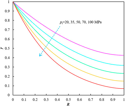
FIGURE 1. The effects of initial reservoir pressure on γ vs. R relationships (T = 90°C and γ_g = 0.6).10 Data Availability Statement [not available in Crossref]

FIGURE 2

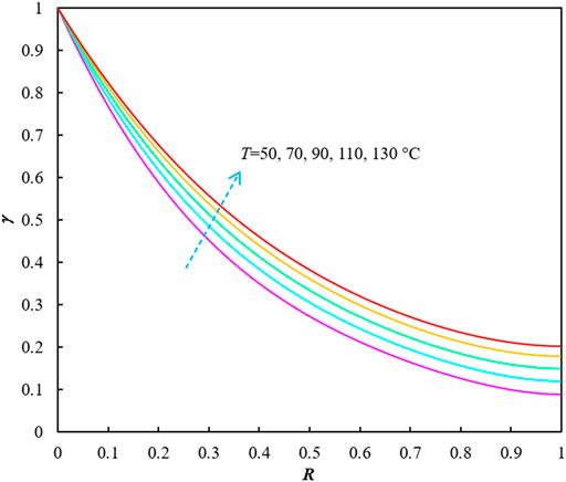
FIGURE 2. The effects of reservoir temperature on γ vs. R relationships (p_i = 70 MPa and γ_g = 0.6).

FIGURE 3

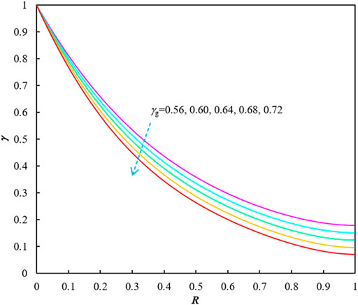
FIGURE 3. The effects of gas gravity on γ vs. R relationships (p_i = 70 MPa and T = 90°C).

Since γ and R are both monotonic functions of pressure and γ decreases monotonically with R, the nonlinear relationship between γ and R can be readily represented by a high order polynomial:

$\gamma \left(p\right)={\displaystyle \sum _{i=0}^n{d}_i\cdot {\left[R\left(p\right)\right]}^i}=d_0+d_1\cdot R+d_2\cdot R^2+d_3\cdot R^3+\mathrm{...}+d_n\cdot R^n(34)$

By substituting Eq. 34 into Eq. 29, we have

$\frac{1}{p_{p_{\mathrm{i}}}}\cdot p_{p_{\mathrm{w}\mathrm{f}}}+\frac{b}{p_{p_{\mathrm{i}}}}\cdot q=\frac{p_{p_{\mathrm{a}\mathrm{v}\mathrm{e}}}}{p_{p_{\mathrm{i}}}}={\displaystyle \sum _{i=0}^n{d}_i\cdot {\left[R\left(p_{\mathrm{a}\mathrm{v}\mathrm{e}}\right)\right]}^i}(35)$

Substituting Eq. 33 into Eq. 35 gives

$\frac{1}{p_{p_{\mathrm{i}}}}\cdot p_{p_{\mathrm{w}\mathrm{f}}}={\displaystyle \sum _{i=0}^n{d}_i\cdot {\left(\frac{G_{\mathrm{p}}}{G}\right)}^i}-\frac{b}{p_{p_{\mathrm{i}}}}\cdot q(36)$

Eq. 36 reveals the relationship between p_wf, q, and G_p during BDF. The left side of Eq. 36 is the measurable variable denoted by “Y” dependent on the bottomhole pressure p_wf, and the right side is termed the estimated variable denoted by “Y_e” where the production rate q and cumulative gas production G_p are measurable production data, nonetheless the gas reserves G and BDF constants b are unknown.

$Y\left(p_{\mathrm{w}\mathrm{f}}\right)=\frac{1}{p_{p_{\mathrm{i}}}}\cdot p_{p_{\mathrm{w}\mathrm{f}}}(37)$

$Y_{\mathrm{e}}\left(G_p,q;G,b\right)={\displaystyle \sum _{i=0}^n{d}_i\cdot {\left(\frac{G_{\mathrm{p}}}{G}\right)}^i}-\frac{b}{p_{p_{\mathrm{i}}}}\cdot q(38)$

The observed values of Y and the estimated values of Y_e are equal in the BDF stage, therefore the production data analysis (p_wf, q, and G_p) of a gas well can be transformed into seeking the optimal combination of (G, b) that minimizes the overall difference between the measurable variable Y and its estimated variable Y_e. This optimization problem can be summarized as:

$\begin{array}{l}\min \mathrm{s}\mathrm{u}\mathrm{m}\left[{\left(Y_{\mathrm{e}}-Y\right)}^2\right]\\ \begin{array}{cc}s.t.& \{\begin{array}{l}G>{\left(G_{\mathrm{p}}\right)}_{\max }\hfill \\ b>0\hfill \end{array}\end{array}\end{array}(39)$

The problem can be solved by the computer programming according to the optimization method without any iterative process. There are three useful functions (“fmincon,” “nlinfit,” and “lsqnonlin”) in Matlab capable of finding the optimal solution to the optimization problem represented by Eq. 39. And they can all generate the desirable results. The last two are adopted in the paper. The resulting gas reserves G reflects the drainage volume controlled by the gas well, while the BDF constant b embodies the deliverability of the gas well. The smaller the value of b, the stronger the production capacity. After determining the optimal G and b, further performance analyses can also be performed such as estimation of average formation pressure, production prediction, and so on. This new optimization-based method for the explicit production data analysis of gas wells is abbreviated to “OBM-EPDA” in the paper. Several examples are used to illustrate its applicability and validity in the ensuing paragraphs.

Case Studies

Cases 1 to 3 are numerical examples where the production data are generated by the numerical simulator; Case 4 is a field example that has been analyzed in the literature. We employ Sutton (2005), Sutton (2007) formulas to estimate the pseudo-critical temperature T_pc and pseudocritical pressure p_pc of the natural gas. The gas viscosity μ can be calculated by the empirical equations presented by Londono et al. (2002), Londono et al. (2005), and the Z-factor and gas compressibility C_g can be determined by the equation of state developed by Hall and Yarborough (1973).

For the numerical examples, we set the gas molecular weight of 17.378400 g/mol (γ_g = 0.6), then Sutton (2005), Sutton (2007) formulas give a pseudo-critical temperature of 197.142 K and a pseudocritical pressure of 4.600 MPa. The initial reservoir pressure is 70 MPa and the formation temperature is 90°C with g (p_i) of 49.167 MPa. The radial grids with a grid number of “300 × 120×1” are used to simulate the single-phase gas flow. The gas well is located in the center of the gas reservoir with a boundary radius of 405 m and a formation thickness of 6 m. Table 1 shows the relevant property parameters of the gas reservoir and natural gas for numerical examples.

TABLE 1

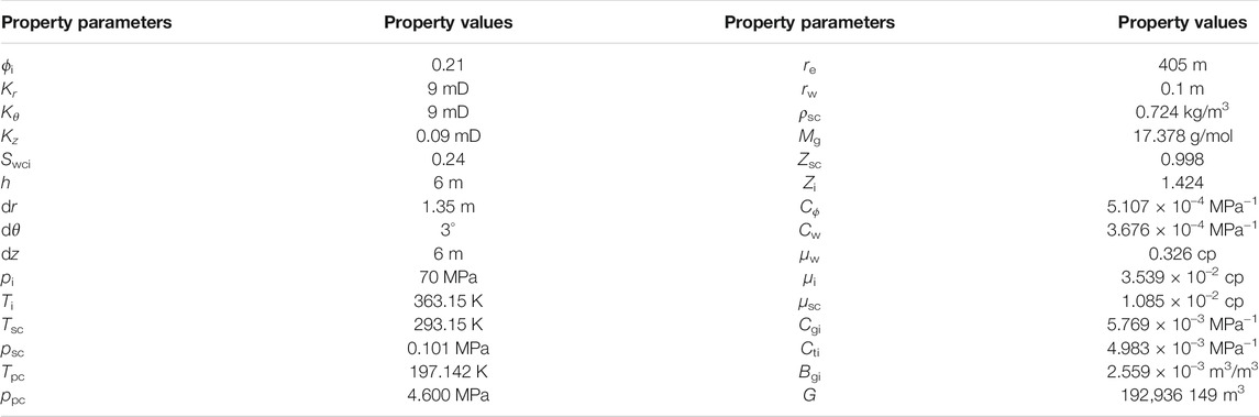
TABLE 1. Property parameters for numerical simulations.

Figure 4 shows the relationship between pseudopressure p_p defined in Eq. 5 and pressure, and the relation of the elastic effect function g(p) defined in Eq. 17 to pressure. The relationship curve of γ(p) vs. R(p) is displayed in Figure 5 where the dotted line represents the γ vs. R relationship generated by the polynomial γ_pol, and ε denotes the fitting error. In practice, Figure 5 can be determined before sorting out the production data of the gas well because the γ vs. R relationship is merely dependent on the properties of the production system (original pressure, temperature, and gas properties) while independent of the production conditions.

$\gamma \approx {\gamma }_{\mathrm{p}\mathrm{o}\mathrm{l}}=4.626681\times {10}^{-1}{R}^4-1.501173R^3+2.399663R^2-2.212882R+1(40)$

$\epsilon =\frac{{\gamma }_{\mathrm{p}\mathrm{o}\mathrm{l}}-\gamma }{\gamma }\times 100\%(41)$

FIGURE 4

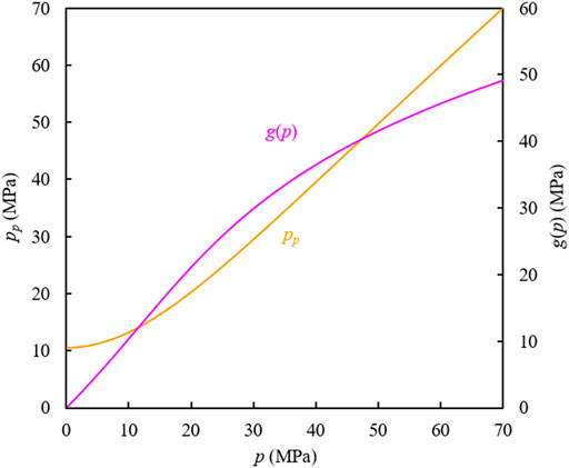
FIGURE 4. p_p and g(p) vs. p for numerical cases.

FIGURE 5

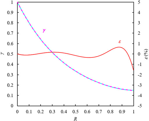
FIGURE 5. γ and ε vs. R for numerical cases.

Case 1: Constant BHP Condition

Case 1 is characterized by the constant BHP of 44.4363 MPa and the production profile within 2000 days is shown in Figure 6A).

FIGURE 6

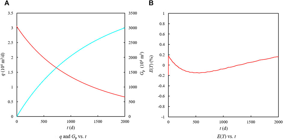
FIGURE 6. q, G_p and E(Y) vs. t for the constant-BHP case.

By solving Eq. 39, we have “G = 1.945959 × 10⁸ m³ and b = 8.504859 MPa⋅(10⁴ m³/d)⁻¹” with a reserves error of 0.860%. Then the estimated variable Y_e defined in Eq. 38 can be calculated. Figure 6B) shows the changes in the difference between Y_e and Y over time, where E(Y) is defined as:

$E\left(Y\right)=\frac{Y_{\mathrm{e}}-Y}{Y}\times 100\%(42)$

As can be seen from Figure 6B), the absolute value of E(Y) is less than 1% during the whole production period, which shows that the values of G and b estimated by the optimization method meet the dynamic material balance equation and the estimations are reliable.

Case 2: Constant Rate Condition

The production schedule of the gas well for Case 2 is changed to the constant rate of 1.5 × 10⁴ m³/d, and the changes in bottomhole pressure and cumulative gas production with time are shown in Figure 7A).

FIGURE 7

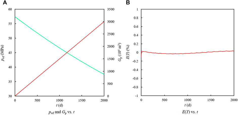
FIGURE 7. p_wf, G_p and E(Y) vs. t for the constant-rate case.

The calculation results of OBM-EPDA that minimizes the differences between Y and Y_e are: G = 1.944803 × 10⁸ m³ and b = 8.471493 MPa⋅(10⁴ m³/d)⁻¹ with a reserves error of 0.800%. Figure 7B) illustrates the corresponding estimation error of Y which demonstrates the effectiveness of OBM-EPDA for the constant-rate production system.

Case 3: Variable-Rate and Variable-BHP Conditions

The production schedule fluctuations of the gas well are simulated by repeatedly modifying the BHP and production rate specifications. The production history of Case 3 is shown in Figure 8A) and Figure 8B).

FIGURE 8

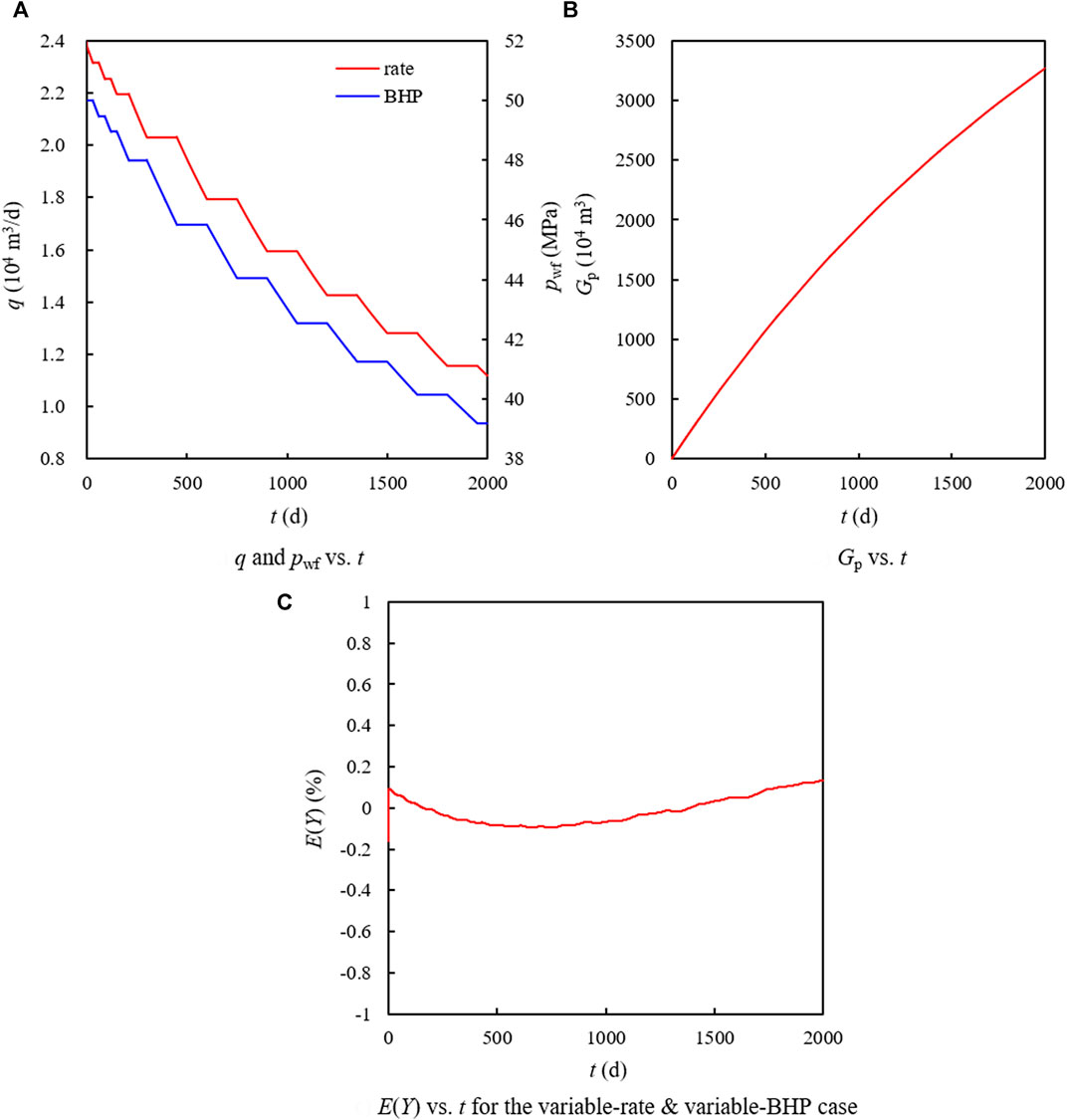
FIGURE 8. The profiles of production rate, BHP, G_p and E(Y) for the variable-rate and variable-BHP case.

For the variable-rate and variable-BHP case, the proposed method gives the gas in place of 1.946829 × 10⁸ m³ and the BDF constant of 8.494877 MPa⋅(10⁴ m³/d)⁻¹ with an error in G of 0.905%. The error statistics of measurable variable Y are displayed in Figure 8C) which indicates the accuracy of the estimated results and the capability of OBM-EPDA to analyze the variable-rate and variable-BHP data.

The optimization-based method for the explicit production data analysis of gas wells (OBM-EPDA) provides the accurate estimates of reserves and boundary dominated flow constants for all the above three numerical examples, and the error statistics also prove the effectiveness and applicability of this method for various gas production systems under the BDF condition. It’s found that the values of b in the three examples have little difference, which shows that the production capacity of the gas well almost remains unaltered despite the changes in production schedule for Cases 1 through 3. OBM-EPDA does not need to iteratively calculate the material balance pseudotime function and can be applied to the complex production system as long as the production data meet the BDF condition, that is, the dynamic material balance equation (DMBE) hold true. A field example that has been widely analyzed is used to further demonstrate the validity and practicability of the presented method in the following paragraphs.

Case 4: Field Case - Gas Well A

Case 4 is taken from a gas reservoir example analyzed by Fetkovich et al. (1987) and Fraim and Wattenbarger (1987). The initial reservoir pressure of Well A in West Virginia is 28.785612 MPa (=4,175 psi) and the formation temperature is 71.11°C. The bottomhole pressure presented by Fetkovich et al. (1987) is 3.447379 MPa (=500 psi), nevertheless Fraim and Wattenbarger (1987) adjusted the BHP to 4.895278 MPa (=710 psi) for the determination of pseudotime. We glean the cumulative production data of the well from Mohammed and Enty (2013) and Alom et al. (2017).

On the basis of the gas gravity of 0.57, the pseudo-critical parameters are determined by Sutton (2005, 2007) correlations (Sutton, 2005; Sutton, 2007), that is, p_pc = 4.605 MPa and T_pc = 191.219 K. The reservoir parameters of Well A are shown in Table 2.

TABLE 2

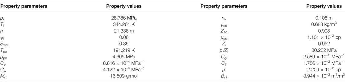
TABLE 2. Reservoir and gas properties for the field case.

Figure 9 shows the changes in p_p and g(p) with pressure p. The relationship between γ and R is displayed in Figure 10 in which the polynomial represented by the dotted line is given by

$\gamma \approx {\gamma }_{\mathrm{p}\mathrm{o}\mathrm{l}}=2.898659\times {10}^{-1}{R}^4-5.778683\times {10}^{-1}{R}^3+9.153651\times {10}^{-1}{R}^2-1.271014R+1(43)$

FIGURE 9

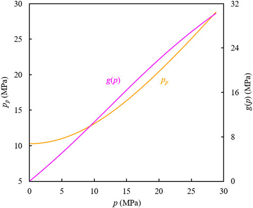
FIGURE 9. p_p and g(p) vs. p for the field case.

FIGURE 10

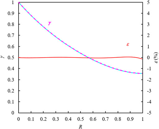
FIGURE 10. λ and ε vs. R for the field case.

Figure 11 shows the production history of Well A, which indicates the frequent fluctuations in production rate and even in BHP.

FIGURE 11

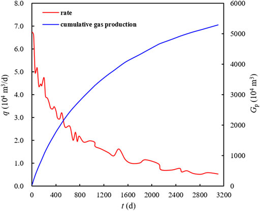
FIGURE 11. Production history of Well A for the field case.

Referring to the practices of most researchers, we take p_wf to be 4.895278 MPa and obtain the analysis results by using OBM-EPDA to minimize the overall difference between Y and Y_e, i.e., G = 7.136728 × 10⁷ m³ and b = 2.960034 MPa⋅(10⁴ m³/d)⁻¹. The error statistics of the measurable variable Y are shown in Figure 12A).

FIGURE 12

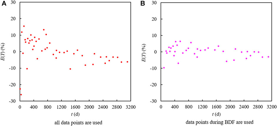
FIGURE 12. E(Y) vs. t for the field case (p_wf = 4.895278 MPa).

The researcher can set a threshold value for E(Y), such as 10%, to determine whether the corresponding data points meet the boundary dominated flow condition (Eq. 28). Those data points not subject to the BDF condition (i.e., E(Y) > 10%), therefore, ought to be removed. It is not difficult to observe from Figure 12A) that the differences between the observed variable and the estimated variable at some data points exceed 10% especially for early period, an indication that these points may not satisfy the BDF condition. After excluding them, the analysis results of OBM-EPDA obtained by using the remaining data are: G = 7.522597 × 10⁷ m³ and b = 3.167751 MPa⋅(10⁴ m³/d)⁻¹ with all the values of E(Y) less than 10% as shown in Figure 12B).

The exclusion of outliers from the target data contributes much to boosting the analyst’s confidence in data selection and thus enhances the confidence level of the performance analysis. The error estimates in Figure 12B), for instance, are superior to the results when all data points are used as illustrated in Figure 12A). The error analysis given by OBM-EPDA helps researchers to judge whether the data points in the evaluation period meet the BDF condition, so as to perform more reasonable production data analysis and improve the reliability of the analysis results.

Table 3 lists the analysis results of the field example in the existing literature based on different methods. The estimated values of G and b by OBM-EPDA are slightly different from them and most consistent with the results presented by Blasingame and Lee (1988). It is worth mentioning that the estimates of G and b have certain uncertainty since the compressibilities of rock and bound water and the pseudo-critical properties of the natural gas are determined by empirical formulas instead of measurements; nonetheless, the error analysis in this paper can improve the reliability of the research results. Therefore, the authors have full confidence in the calculation results of the explicit method in the paper.

TABLE 3

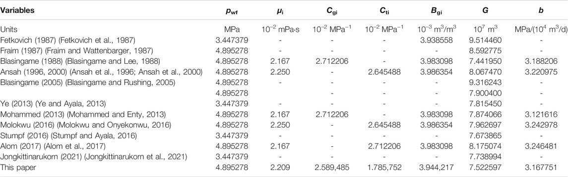
TABLE 3. Comparison with existing calculation results for the field case.

Conclusion

Based on the gas flow equation for BDF derived from the mathematical model of gas seepage and the SMBE of a gas reservoir, this paper strictly proves the dynamic material balance equation. Then on this basis, an optimization-based method for the explicit production data analysis of gas wells (OBM-EPDA) is proposed by introducing the pseudopressure level function γ(p) and the recovery factor function R(p). The following understandings and conclusions are drawn:

1) The relationship between γ and R is an inherent attribute of a gas reservoir which is dependent on the initial reservoir pressure p_i, reservoir temperature T, and gas pseudocritical parameters (T_pc, p_pc), but independent of production schedules or quantity of production data.

2) A polynomial function can be employed to delineate the nonlinearity of γ vs. R relationship and the quartic polynomial is generally accurate enough.

3) OBM-EPDA can quickly and efficiently analyze the production data of a gas well under constant BHP, constant production rate, and variable-rate/variable-BHP conditions for estimation of gas reserves G and BDF constant b, and thus provide information about the control area and production capacity of the gas well.

4) The error of the observed Y at each data point obtained by the proposed method allows reservoir engineers to identify the appropriate data set which ought to satisfy the BDF condition, and hence enhance the credibility of the analysis results.

5) OBM-EPDA avoids any iterative process and is proved to be effective in analyzing the variable rate and variable BHP data, which overcomes the respective defects of existing implicit and explicit PDA methods.

Data Availability Statement

The original contributions presented in the study are included in the article/Supplementary Material, further inquiries can be directed to the corresponding author.

Author Contributions

LZ: Conceptualization, Methodology, Software, Validation, Formal Analysis, Investigation, Writing—Original Draft. YL: Resources, Supervision, Writing—Review and Editing. XS: Supervision, Project administration. MW: Writing—Review and Editing. YY: Software. YH: Software, Validation. ZZ: Data Curation, Visualization. CL: Formal Analysis.

Funding

This work is supported by the National Science and Technology Major Project of China (Grant No. 2017ZX05030003 and 2016ZX05015002). This study has been supported by the Department of Middle East E and P and the Department of Asia-Pacific E and P, Research Institute of Petroleum Exploration and Development (RIPED), PetroChina.

Conflict of Interest

LZ, YL, XS, YY, ZZ are employed by Research Institute of Petroleum Exploration and Development, PetroChina. Y-xH is employed by Bohai Oilfield Research Institute, Tianjin Branch of CNOOC (China) Limited. CL is employed by CNPC Bohai Drilling Engineering Company Limited. The authors declare that this study received funding from Research Institute of Petroleum Exploration and Development (RIPED), PetroChina. The funder had the following involvement in the study: decision to publish.

Publisher’s Note

All claims expressed in this article are solely those of the authors and do not necessarily represent those of their affiliated organizations, or those of the publisher, the editors and the reviewers. Any product that may be evaluated in this article, or claim that may be made by its manufacturer, is not guaranteed or endorsed by the publisher.

Acknowledgments

We gratefully acknowledge financial support from RIPED. Our thanks also go to Jinyu Guo and Lang Li for revision suggestions.

References

Agarwal, R. G., Gardner, D. C., Kleinsteiber, S. W., and Fussell, D. D. (1998). Analyzing Well Production Data Using Combined Type Curve and Decline Curve Analysis Concepts. Louisiana 2, 585–598. doi:10.2118/49222-MS

CrossRef Full Text | Google Scholar

Agarwal, R. G., Gardner, D. C., Kleinsteiber, S. W., and Fussell, D. D. (1999). Analyzing Well Production Data Using Combined-Type-Curve and Decline-Curve Analysis Concepts. SPE Reservoir Eval. Eng. 2 (5), 478–486. doi:10.2118/57916-PA

CrossRef Full Text | Google Scholar

Ahmed, T., and Meehan, D. N. (2012). Advanced Reservoir Management and Engineering. 2nd Edition. Waltham, MA: Gulf Professional Publishing, 301–325.

Google Scholar

Alom, M. S., Tamim, M., and Rahman, M. M. (2017). Decline Curve Analysis Using Rate Normalized Pseudo-cumulative Function in a Boundary Dominated Gas Reservoir. J. Pet. Sci. Eng. 150, 30–42. doi:10.1016/j.petrol.2016.11.006

CrossRef Full Text | Google Scholar

Ansah, J., Knowles, R. S., and Blasingame, T. A. (1996). “A Semi-analytic (P/z) Rate-Time Relation for the Analysis and Prediction of Gas Well Performance,” in presented at the SPE Mid-Continent Gas Symposium, Amarillo, Texas, 28-30 April, 1–19. doi:10.2118/35268-MS

CrossRef Full Text | Google Scholar

Ansah, J., Knowles, R. S., and Blasingame, T. A. (2000). A Semi-analytic (P/z) Rate-Time Relation for the Analysis and Prediction of Gas Well Performance. SPE Reservoir Eval. Eng. 3 (6), 525–533. doi:10.2118/66280-PA

CrossRef Full Text | Google Scholar

Arps, J. J. (1945). Analysis of Decline Curves. Trans. AIME 160 (1), 228–247. doi:10.2118/945228-G

CrossRef Full Text | Google Scholar

Behmanesh, H., Mattar, L., Thompson, J. M., Anderson, D. M., Nakaska, D. W., and Clarkson, C. R. (2018). Treatment of Rate-Transient Analysis during Boundary-Dominated Flow. SPE J. 23 (4), 1145–1165. doi:10.2118/189967-PA

CrossRef Full Text | Google Scholar

Blasingame, T. A., Johnston, J. L., and Lee, W. J. (1989). “Type-Curve Analysis Using the Pressure Integral Method,” in presented at the SPE California Regional Meeting, Bakersfield, California, 5-7 April, 525–538. doi:10.2118/18799-MS

CrossRef Full Text | Google Scholar

Blasingame, T. A., and Lee, W. J. (1986). “Variable-Rate Reservoir Limits Testing,” in Permian Basin Oil and Gas Recovery Conference, Midland, Texas, 13-15 March, 361–369. doi:10.2118/15028-MS

CrossRef Full Text | Google Scholar

Blasingame, T. A., and Lee, W. J. (1988). ““Variable-rate Reservoir Limits Testing of Gas wells,”,” in presented at the SPE Gas Technology Symposium, Dallas, Texas, 13-15 June, 43–56. doi:10.2118/17708-MS

CrossRef Full Text | Google Scholar

Blasingame, T. A., McCray, T. L., and Lee, W. J. (1991). ““Decline Curve Analysis for Variable Pressure Drop/variable Flowrate Systems,”,” in presented at the SPE Gas Technology Symposium, Houston, Texas, 22-24 January, 1–17. doi:10.2118/21513-MS

CrossRef Full Text | Google Scholar

Blasingame, T. A., and Rushing, J. A. (2005). “A Production-Based Method for Direct Estimation of Gas in Place and Reserves,” in presented at the SPE Eastern Regional Meeting, Morgantown, West Virginia, 14-16 September, 1–17. doi:10.2118/98042-MS

CrossRef Full Text | Google Scholar

Buba, I. M. (2003). “Direct Estimation of Gas Reserves Using Production Data,” (College Station, TX: Texas A&M University). Master’s Thesis.

Google Scholar

Callard, J. G., and Schenewerk, P. A. (1995). “Reservoir Performance History Matching Using Rate/cumulative Type-Curves,,” in presented at the SPE Annual Technical Conference and Exhibition, Dallas, Texas, 22-25 October, 947–956. doi:10.2118/30793-MS

CrossRef Full Text | Google Scholar

Canard, J. G. (1994). “Reservoir Performance History Matching Using Type-Curves,” (Baton Rouge: Louisiana State University). Dissertation.

Google Scholar

Carter, R. D. (1981). “Characteristic Behavior of Finite Radial and Linear Gas Flow Systems - Constant Terminal Pressure Case,” in SPE/DOE Low Permeability Gas Reservoirs Symposium, Denver, Colorado, 27-29 May, 527–539. doi:10.2118/9887-MS

CrossRef Full Text | Google Scholar

Carter, R. D. (1985). Type Curves for Finite Radial and Linear Gas-Flow Systems: Constant-Terminal-Pressure Case. Soc. Pet. Eng. J. 25 (5), 719–728. doi:10.2118/12917-PA

CrossRef Full Text | Google Scholar

Chaudhry, A. U. (2003). Gas Well Testing Handbook. Burlington, MA: Gulf Professional Publishing, 340–353.

Google Scholar

Fetkovich, M. J. (1980). Decline Curve Analysis Using Type Curves. J. Pet. Tech. 32 (6), 1065–1077. doi:10.2118/4629-PA

CrossRef Full Text | Google Scholar

Fetkovich, M. J., Vienot, M. E., Bradley, M. D., and Kiesow, U. G. (1987). Decline Curve Analysis Using Type Curves: Case Histories. SPE Formation Eval. 2 (4), 637–656. doi:10.2118/13169-PA

CrossRef Full Text | Google Scholar

Fraim, M. L., and Wattenbarger, R. A. (1987). Gas Reservoir Decline-Curve Analysis Using Type Curves with Real Gas Pseudopressure and Normalized Time. SPE Formation Eval. 2 (4), 671–682. doi:10.2118/14238-PA

CrossRef Full Text | Google Scholar

Hall, K. R., and Yarborough, L. (1973). A New Equation of State for Z-Factor Calculations. Oil Gas J. 71 (25), 82–85. Available at: https://www.researchgate.net/publication/284299884.

Google Scholar

Jongkittinarukorn, K., Last, N., Escobar, F. H., and Srisuriyachai, F. (2021). A Straight-Line DCA for a Gas Reservoir. J. Pet. Sci. Eng. 201, 108452. doi:10.1016/j.petrol.2021.108452

CrossRef Full Text | Google Scholar

Kamal, M. M. (2009). Transient Well Testing. Richardson, TX: Society of Petroleum Engineers.

Google Scholar

Knowles, R. S. (1999). “Development and Verification of New Semi-analytical Methods for the Analysis and Prediction of Gas Well Performance,” (College Station, TX: Texas A&M University). Master’s Thesis.

Google Scholar

Londono, F. E., Archer, R. A., and Blasingame, T. A. (2005). Correlations for Hydrocarbon Gas Viscosity and Gas Density - Validation and Correlation of Behavior Using a Large-Scale Database. SPE Reservoir Eval. Eng. 8 (6), 561–572. doi:10.2118/75721-PA

CrossRef Full Text | Google Scholar

Londono, F. E., Archer, R. A., and Blasingame, T. A. (2002). “Simplified Correlations for Hydrocarbon Gas Viscosity and Gas Density - Validation and Correlation of Behavior Using a Large-Scale Database,” in presented at the SPE Gas Technology Symposium, Calgary, Alberta, 30 April-2 May, 1–16. doi:10.2118/75721-MS

CrossRef Full Text | Google Scholar

Mattar, L., and Anderson, D. (2005). “Dynamic Material Balance(Oil or Gas-In-Place without Shut-Ins,” in presented at the Canadian International Petroleum Conference, Calgary, Alberta, 7-9 June, 1–9. doi:10.2118/2005-113

CrossRef Full Text | Google Scholar

Mattar, L., and Anderson, D. M. (2003). “A Systematic and Comprehensive Methodology for Advanced Analysis of Production Data,” in SPE Annual Technical Conference and Exhibition, Denver, Colorado, October, 1-14, 5–8. doi:10.2118/84472-MS

CrossRef Full Text | Google Scholar

Mattar, L., Anderson, D., and Stotts, G. (2006). Dynamic Material Balance-Oil-Or Gas-In-Place without Shut-Ins. J. Can. Pet. Tech. 45 (11), 7–10. doi:10.2118/06-11-TN

CrossRef Full Text | Google Scholar

Mattar, L., and McNeil, R. (1998). The "flowing" Gas Material Balance. J. Can. Pet. Tech. 37 (2), 52–55. doi:10.2118/98-02-06

CrossRef Full Text | Google Scholar

Mattar, R., and McNeil, R. (1995). “The "Flowing" Material Balance Procedure,” in Annual Technical Meeting, Banff in Alberta, 14-17 May, 1–6. doi:10.2118/95-77

CrossRef Full Text | Google Scholar

Meunier, D. F., Kabir, C. S., and Wittmann, M. J. (1984). “Gas Well Test Analysis: Use of Normalized Pressure and Time Functions,” in presented at the SPE Annual Technical Conference and Exhibition, Houston, Texas, 16-19 September, 1–16. doi:10.2118/13082-MS

CrossRef Full Text | Google Scholar

Meunier, D. F., Kabir, C. S., and Wittmann, M. J. (1987). Gas Well Test Analysis: Use of Normalized Pseudovariables. SPE Formation Eval. 2 (4), 629–636. doi:10.2118/13082-PA

CrossRef Full Text | Google Scholar

Moghadam, S., Jeje, O., and Mattar, L. (2011). Advanced Gas Material Balance in Simplified Format. J. Can. Pet. Tech. 50 (1), 90–98. doi:10.2118/139428-PA

CrossRef Full Text | Google Scholar

Moghadam, S., Jeje, O., and Mattar, L. (2009). “Advanced Gas Material Balance, in Simplified Format,” in presented at the Canadian International Petroleum Conference, Calgary, Alberta, 16-18 June, 1–10. doi:10.2118/2009-149

CrossRef Full Text | Google Scholar

Mohammed, S., and Enty, G. S. (2013). “Analysis of Gas Production Data Using Flowing Material Balance Method,” in Annual International Conference and Exhibition, Lagos, Nigeria, 5-7 August, 1–22. doi:10.2118/167504-MS

CrossRef Full Text | Google Scholar

Molokwu, V. C., and Onyekonwu, M. O. (2016). “A Nonlinear Flowing Material Balance for Analysis of Gas Well Production Data,” in Annual International Conference and Exhibition, Lagos, Nigeria, 2-4 August, 1–22. doi:10.2118/184258-MS

CrossRef Full Text | Google Scholar

Palacio, J. C., and Blasingame, T. A. (1993). UNAVAILABLE - Decline-Curve Analysis with Type Curves - Analysis of Gas Well Production Data. Denver, Colorado: Society of Petroleum Engineers, 26–28. April, 1-30. doi:10.2118/25909-MS

CrossRef Full Text | Google Scholar

Russell, D. G., Goodrich, J. H., Perry, G. E., and Bruskotter, J. F. (1966). Methods for Predicting Gas Well Performance. J. Pet. Tech. 18 (1), 99–108. doi:10.2118/1242-PA

CrossRef Full Text | Google Scholar

Spivey, J. P., and Lee, W. J. (2013). Applied Well Test Interpretation. Richardson, TX: Society of Petroleum Engineers.

Google Scholar

Stumpf, T. N., and Ayala, L. F. (2016). Rigorous and Explicit Determination of Reserves and Hyperbolic Exponents in Gas-Well Decline Analysis. SPE J. 21 (5), 1843–1857. doi:10.2118/180909-PA

CrossRef Full Text | Google Scholar

Sun, H. D. (2015). Advanced Production Decline Analysis and Application. Waltham, MA: Gulf Professional Publishing, 95–167.

Google Scholar

Sutton, R. P. (2005). “Fundamental PVT Calculations for Associated and Gas-Condensate Natural Gas Systems,” in presented at the SPE Annual Technical Conference and Exhibition, Dallas, Texas, 9-12 October, 1–20. doi:10.2118/97099-MS

CrossRef Full Text | Google Scholar

Sutton, R. P. (2007). Fundamental PVT Calculations for Associated and Gas/condensate Natural-Gas Systems. SPE Reservoir Eval. Eng. 10 (3), 270–284. doi:10.2118/97099-PA

CrossRef Full Text | Google Scholar

Wang, Y., and Ayala, L. F. (2020). Explicit Determination of Reserves for Variable-Bottomhole-Pressure Conditions in Gas Rate-Transient Analysis. SPE J. 25 (1), 369–390. doi:10.2118/195691-PA

CrossRef Full Text | Google Scholar

Ye, P., and Ayala H., L. F. (2012). A Density-Diffusivity Approach for the Unsteady State Analysis of Natural Gas Reservoirs. J. Nat. Gas Sci. Eng. 7, 22–34. doi:10.1016/j.jngse.2012.03.004

CrossRef Full Text | Google Scholar

Ye, P., and Ayala, L. (2013). Straightline Analysis of Flow Rate vs. Cumulative-Production Data for the Explicit Determination of Gas Reserves. J. Can. Pet. Tech. 52 (4), 296–305. doi:10.2118/165583-PA

CrossRef Full Text | Google Scholar

Zhang, L., He, Y., Guo, C., and Yu, Y. (2021). Dynamic Material Balance Method for Estimating Gas in Place of Abnormally High-Pressure Gas Reservoirs. Lithosphere 2021, 6669012. doi:10.2113/2021/6669012

CrossRef Full Text | Google Scholar

Zhang, L. X., Guo, C. Q., and Jiang, H. (2019). Gas in Place Determination by Material Balance-Quasipressure Approximation Condition Method. Acta Petrolei Sinica 40 (3), 337–349. doi:10.7623/syxb201903008

CrossRef Full Text | Google Scholar