 Huajin Li
 Jiahao Deng
 Peng Feng1
 Dimuthu D. K. Arachchige
95% of researchers rate our articles as excellent or good
Learn more about the work of our research integrity team to safeguard the quality of each article we publish.
Find out more
ORIGINAL RESEARCH article
Front. Energy Res. , 26 October 2021
Sec. Wind Energy
Volume 9 - 2021 | https://doi.org/10.3389/fenrg.2021.780928
This article is part of the Research Topic Advanced Anomaly Detection Technologies and Applications in Energy Systems View all 64 articles
To maximize energy extraction, the nacelle of a wind turbine follows the wind direction. Accurate prediction of wind direction is vital for yaw control. A tandem hybrid approach to improve the prediction accuracy of the wind direction data is developed. The proposed approach in this paper includes the bilinear transformation, effective data decomposition techniques, long-short-term-memory recurrent neural networks (LSTM-RNNs), and error decomposition correction methods. In the proposed approach, the angular wind direction data is firstly transformed into time-series to accommodate the full range of yaw motion. Then, the continuous transformed series are decomposed into a group of subseries using a novel decomposition technique. Next, for each subseries, the wind directions are predicted using LSTM-RNNs. In the final step, it decomposed the errors for each predicted subseries to correct the predicted wind direction and then perform inverse bilinear transformation to obtain the final wind direction forecasting. The robustness and effectiveness of the proposed approach are verified using data collected from a wind farm located in Huitengxile, Inner Mongolia, China. Computational results indicate that the proposed hybrid approach outperforms the other single approaches tested to predict the nacelle direction over short-time horizons. The proposed approach can be useful for practical wind farm operations.
Wind energy generation is expanding with about 12% of world’s electricity to be supplied by 2020 (Kodama and Burls 2019). Compared with the traditional form of power generation, wind energy has the advantages of zero pollution and low operation cost. Hence, it has become one of the fastest growing renewable energy power supplies globally (Duan et al., 2021).
Although it has obvious advantages over others, wind energy still faces technical challenges due to the characteristics of chaos, randomness, and intermittence which make the wind data complex. The wind direction is one of the most complex aspect of the wind data due to its high dynamics in both spatial and temporal domains. To follow the wind direction, the nacelle of a wind turbine orientes the controlling of yaw and maximizes the energy output. For most efficient energy extraction, the nacelle orientation of a wind turbine needs to agree with wind direction which calls for accurate and prediction of the wind direction (Hu et al., 2016).
According to literature review, statistical approaches based on meteorological and geographic information are widely applied to forecast wind direction (Mcwilliams and Sprevak 1982; Castino et al., 1998; Erdem and Shi 2011). Liu et al. (2010) applied a neural Kriging method to spacially estimate the distribubiton of wind directions. Erdem and Shi (2011) developed autoregressive moving average (ARMA) model to forecast the short-term wind directions. Masseran et al. (2013) used a mixture of Von Mises models to fit the wind direction series.
Therefore, machine learning adoptions for wind direction forecasting have evolved from the classic approach to deep learning, which is then improved in this study (Mohandes et al., 2004; Bilgili et al., 2007). In the wind direction forecasting sector, Zhou et al. (2011) selected least-square support vector machines (LS-SVM) to predict the wind directions. Tagliaferri et al. (2015) developed artificial neural networks to forecast the short-term wind directions. Khosravi et al. (2018) developed an adaptive neuro-fuzzy inference system to predict the wind directions. Amin et al. (2018) improved the wind direction forecasting using the echo state network (ESN) which is a deep-learning algorithm. Tang et al. (2021) integrated the ESN network with IFPA optimization algorithm and developed a two-step deep-learning wind direction framework.
Considering the complexity and high dynamics of the wind direction series, additional measures are essential to study in the pattern inside. Even though deep learning algorithms have achieved promising results in the field of time-series prediction, it is still challenging for a single deep-learning approach to adapt all wind direction patterns. To further improve the prediction performance, hybrid prediction models are considered to be the mainstream since last year. The signal decomposition is one of the most popular components within the hybrid models published. It contains wavelet decomposition (Liu et al., 2014), empirical mode decomposition (EMD) (Santhosh et al., 2018), complete ensemble empirical model decomposition (CEEMD) (Zhang et al., 2017), complete EEMD with adaptive noise (CEEMDAN) (Yang and Wang 2018), and the improved CEEMDAN (ICEEMDAN) (Rong et al., 2019). In particular, the ICEEMDAN has demonstrated its superior performance in decomposing a complex signal into a finite number of intrinsic mode functions with transient frequencies. The decomposed subseries contains the detailed characteristics of the signal and can essentially reflect the spatial and temporal patterns of the wind direction series (Kou et al., 2020).
Based on the above considerations, in this research, we propose a new hybrid approach combining ICEEMDAN and error correction methods for short-term wind direction forecasting. First, the angular wind direction data has been transformed via bilinear transformation. Then, the transformed wind direction series are decomposed into a series of relatively simple subseries by the ICEEMDAN modules. Next, the LSTM-RNN is established as the prediction module to predict each sub-series. After that, the prediction errors are obtained and decomposed by ICEEMDAN modules. The statistical ARIMA model is used to predict the error subsequence and compute the prediction error. In the last step, the final prediction of the wind direction is made by summing all predicted subseries together with current predicted error and then transformed into angular data by inverse bilinear transformation.
The major contribution of this research can be summarized as follows: First, the wind direction forecasting system based on ICEEMDAN decomposition, LSTM-RNN and error correction has been proposed; Second, the comparative analysis is performed against other benchmarking deep-learning algorithm; Third, the experiments were performed in different seasons to explore seasonal patterns of wind directions.
The remainder of the manuscript is configured as follows. In Section “dataset description and transformation”, it summarizes the data collection process and patterns inside the wind direction dataset. In Section “methodologies”, it introduces the ICEEMDAN decomposition, LSTM-RNN, error correction, benchmarking deep-learning algorithms, and error correction procedures. The experimental results are provided in Section “experimental results” and the Conclusion is made in Section “conclusions” respectively.
In this study, the data has been collected during the year of 2020 from a wind farm namely Huitengxile wind power plant in Inner Mongolia, Northern China. It is one of the largest wind farms in Asian and it’s located in the suburbs between Chaha’er youyi zhongqi and Ulanqab city. The whole wind farm has multiple wind turbines that are distributed in an open flat grassland which provides rich wind resources. The prevailing wind directions are northwest and southeast which are very stable in recent years. The location and the annual wind rose diagrams has been illustrated in Figure 1 below.
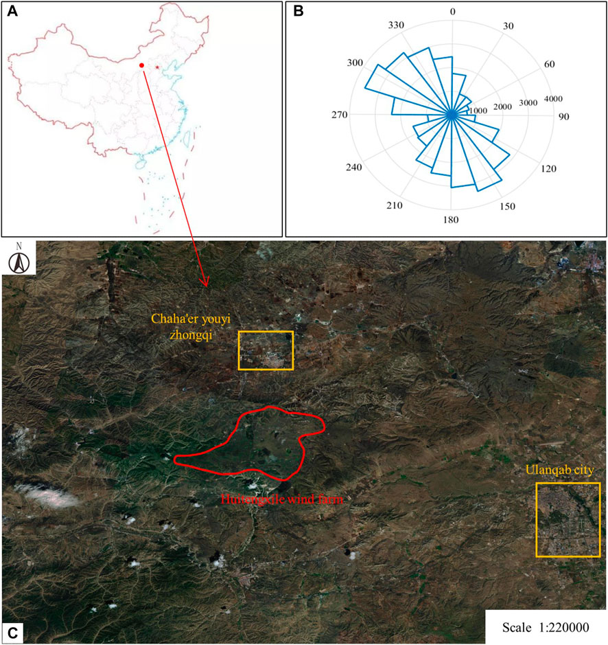
FIGURE 1. Location of the Huitengxile wind farm.
According to Figure 1B, the two prevailing wind directions, around 180° and 315° are visible. The geographic center coordinate is 112°40′E and 41°05′N. It’s annual average wind speed at 10 m height is 7.2 m/s and its annual average wind speed at 40 m height is 8.8 m/s. In the wind farm, the annual average air density is 1.07 kg/m and it contains an effective wind speed of 5–25 m/s with strong stability and high quality.
The data used in this research has been collected by the supervisory control and data acquisition (SCADA) system. Usually, data on more than 100 parameters at 10 s intervals is collected and stored in a SCADA system. The SCADA collected data of individual wind turbines is streamed to a central computer for condition monitoring, performance evaluation, and other forms of analysis.
In this research, the SCADA data collected at 20 wind turbines over the period of 2020 has been analyzed. According to Figure 1B, there are two annual prevailing wind directions and it can be partitioned into four seasons independently as illustrated with the wind roses in Figure 2. In the fall and spring, two prevailing wind directions around 150° and 315°are observed. In the winter and summer, one prevailing wind direction is noted. Since the wind direction data is captured as a discrete angular variable, it needs to be transformed for modeling. A bilinear transformation of the angular wind direction is applied in the next section.
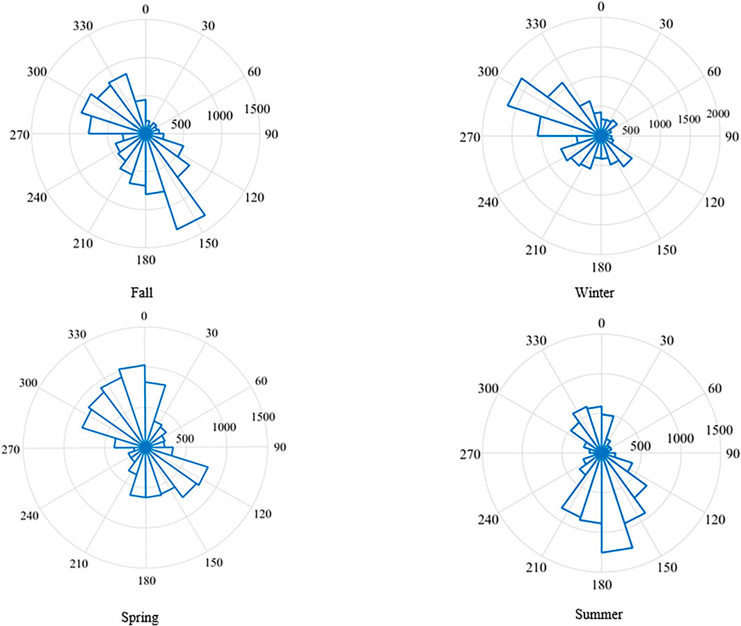
FIGURE 2. Wind rose diagrams for four seasons.
The value of wind direction ranges from 0° to 360°. It is likely that the wind direction may change from the interval, i.e (0°, 10°) to (350°, 360°). Practice shows that bilinear transformation is a better way for transforming discrete wind direction data to continuous data than the sine and cosine transformation (Peng et al., 2020). Geometrically, the two intervals are close to each other and therefore this change would lead to a large prediction error (Bilgili et al., 2007). To avoid such error, transformation of the discrete angular variable into a standardized continuous variable is essential. One option is to use a sine and cosine transformation which is not the best approach due to two variables needed for prediction which enlarges the prediction errors. A better option is to apply a bilinear transformation (Jury 1973).
The bilinear transformation maps the analog plane (s-plane) into the digital plane (z-plane) (Groutage et al., 2003) (see Figure 3). The transformation function, the ratio of two polynomials (Davies 1974), is expressed in Eq. 1.
where: s is the original value of angular variable in s-plane; T is the time interval of the transformation. The bilinear transformation expressed the angular variable between 0° and 360° as continuous and normalized. The inverse bilinear transformation is expressed in Eq. 2.
where: s is the inversed value of angular variable in s-plane; and H(s)z is the transformed angular variable.
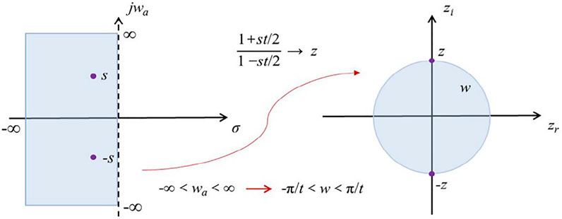
FIGURE 3. Illustration of the bilinear transformation.
Since the wind direction data is noisy, a bilinear transformation function acting as a low-pass filter in the continuous-time domain reduces the noise (Davies 1974). A prediction model developed with the transformed data is more accurate than the model based on the discrete time-series angular data.
The use of deep learning algorithms in regression, multi-class classification, collaborative filtering, and graphic learning is growing (Lecun et al., 2015). The concept of deep learning originates from research in neural networks and it avoids the local optima dilemma. However, any single deep learning algorithms can offer limited extraction of patterns inside the dataset. Hybrid frameworks containing multiple deep learning algorithm is becoming the new mainstream in academia.
In this research, the improved complete ensemble empirical mode decomposition with adaptive noise (ICEEMDAN) is served as the major module in the hybrid forecasting framework. It is considered as an improvement on empirical mode decomposition (EMD) which decomposes the wind directions in the temporal domain (Colominas et al., 2014).
The time-series of wind direction can be expressed as the sum of multiple IMFs and the residual after the ICEEMDAN decomposition which can be expressed in Eq. 3 as follows:
The amplitude energy
where N denotes the total number of sampling points of the jth IMF. Assuming that the energy carried by r(t) can be ignored, the total energy of the transformed direction series can be expressed as Eq. 5 as follows:
To remain the data in the same magnitude, the amplitude of the IMFs is normalized to facilitate the subsequent calculations and the impact of singular data has been reduced. Hence, the energy entropy of the ICEEMDAN framework can be expressed as Eq. 6 below:
Compared with other decomposition methods, the ICEEMDAN can not only reduce the noise in the original time-series data but also reduce the residual spurious pattern problems based by signal overlap. Thus, the decomposed subseries gains more orthogonality among each other and it can provide more accurate reconstruction of the original series.
To integrate the wind direction series with the ICEEMDAN modules, the implementations are introduced as follows (Duan et al., 2021):
Step 1: Compute the local means of realizations using the EMD algorithm described in Eq. 7:
where
Step 2: Compute residual term R1 in the first component using Eq. 8:
Step 3: Compute the first mode at the first stage (k = 1) using Eq. 9:
Step 4: Estimate the second residue as the average of local means of the realizations
Step 5: For the other terms (k = 3, … ,K) of residuals, they can be computed by Eq. 11:
Step 6: Compute the other terms (k = 3, … ,K) of the mode by Eq. 12:
Step 7: Implement step 4 for the next iteration.
For the transformed wind direction series, the IMF components are obtained via the above steps which can be illustrated by the diagram presented in Figure 4.
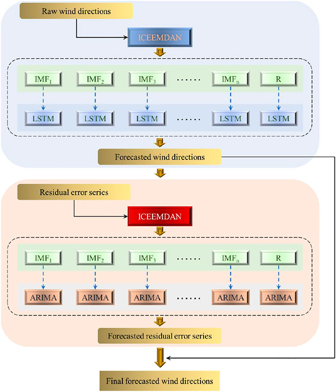
FIGURE 4. Diagrams of ICEEMDAN modules.
A major drawback of the classical deep neural networks is that they do not have memory of the past periods. The time series information such as the past clusters of seasonal patterns and seasonal trend may not be reflected (Lee et al. 1993). Introduced by Hochreiter and Schmidhuber (1997) and Gers et al. (2003), the long-short-term memory recurrent neural network (LSTM-RNN) matches the needs and it is used in this paper to predict wind direction.
The long-short-term memory recurrent neural network (LSTM-RNN) contains units called memory blocks composed of memory cells with self-connections storing temporal states. Each memory block includes an input and output gate. The input gate controls the flow of input data into the cell. The output gate controls the output data flow into the rest of the network (Sak et al. 2014). In addition, the LSTM-RNN has peephole connections (Gers et al. 2003) from its internal cells to the gates in the same cell to learn precise timing of the output. The architecture of LSTM-RNN is illustrated in Figure 5.
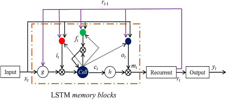
FIGURE 5. Autocorrelation analysis of time-series wind direction data.
With a long-short-term memory recurrent neural network (LSTM-RNN) architecture, the mapping from an input to an output layer is iteratively computed from Eqs 13–18 (Gers et al. 2003).
where: W are the weight matrices (i.e., Wix is the weight matrix from the input to the input layer; Wic, Wfc, Woc are diagonal weight matrices of the peephole connections (Gers et al., 2003)); bi,bf,bo, and bc are the bias vectors; m is the cell output activation vector; sig () is the sigmoid function; i, f, o, and c are the input gate, forget gate, output gate, and cell activation vectors, respectively, with all having the same size as the cell output activation vector m;
Comparative analysis is performed in this research against the other benchmarking popular deep learning algorithms. All algorithms tested here are using the same ICEEMDAN framework as described in Section “Short-term Wind Direction Forecasting using ICEEMDAN”. The benchmarking deep learning algorithms compared includes deep neural network (DNN) (Xu et al., 2018; Sun et al., 2020; Yi and Xu, 2020), deep belief network (DBN) (Ouyang et al., 2019; Li et al., 2020), kernel-based extreme learning machine (KELM) (Li et al., 2018; Ouyang et al., 2018), and gated recurrent unit network (GRU) (Pan et al., 2019; Tang and Zhang, 2019).
The DNN is a fully connected feedforward network that consists of a cascade of multiple layers and hidden units. It’s structure with multiple processing layers enables it to handle highly nonlinear patterns inside the dataset. The deep temporal representations in the temporal domain can be effectively extracted by DNN.
Similar to DNN, the DBN consists of multiple layers of restricted Boltzmann machines (RBMs). It also contains a supervised regression layer stacked on the top of all RMBs for classification or regression tasks. Inside each RBM, it contains an input layer and a hidden layer with hidden-to-all-visible connections.
The ELM is a single hidden layer feedforward network. Instead of conventional back-propagation, it uses Penn-Moore pseudo-inverse to compute the wights between the hidden layer and output layer. The KELM is the improvement of vanilla ELM which uses the kernel matrix to replace the randomly initialized weights between the input layer and output layer. The most popular applied kernel functions include RBF, linear function, and polynomial function.
The GRU is another type of recurrent neural network other than LSTM-RNN proposed by Cho et al. (2014). In a typical GRU unit, it has one less gate than the LSTM unit and consists of two gates: the reset gate and the update gate. Hence, the GRU is also popular in modeling time-series dataset.
To assess prediction accuracy of the proposed deep learning model, four metrics are computed: the MAE [Mean absolute error (Eq. 19)], the MAPE [Mean absolute percentage error (Eq. 20)], the MSE [Mean square error (Eq. 21)], and the RMSE [Root mean square error (Eq. 22)].
where: oj is the jth predicted wind direction; tj is the jth measured wind direction; and N denotes total number of samples.
To improve the forecasting accuracy, the error correction is implemented in this research. First, after the forecasting outcome produced by each LSTM-RNN, the error series E(t) of the training dataset can be computed by comparing the original transformed wind direction series. The step can be expressed in Eq. 23 as follows:
where
The forecasted errors of wind direction series E(t) are oscillatory in the time-series domain (Wasynczuk et al., 1981). The relationship between oscillatory and decaying property of the wind direction errors can be represented by an ARIMA model which predicts the errors. In detail, the ARIMA can be constructed by computing autocorrelation expressed with the autocorrelation factor (ACF) (See. Eq. 24) and the partial autocorrelation factor (PACF)) (See. Eq. 25). Here, Cov() denotes the covariance; Var() denotes the variance; and Corr () denotes the Pearson’s correlation coefficient.
For each IMF, an ARIMA model is developed and then all outcomes of each ARIMA are integrated to obtain the final error series. Last, as illustrated in Figure 4, the final prediction is achieved by Eq. 26 as follows:
where
In this section, computational experience with models predicting wind direction is presented. Wind data from four seasons, spring, summer, fall, and winter are used. Prediction of wind direction is conducted using dataset at 10, 20, and 30 s resolution. The prediction horizons are 2, 5, 10 min, and 1 h. The prediction model is expressed in Eqs 27–29.
where: f(D) represents the whole framework illustrated in Figure 4; Dt-i is the ith lagged vector containing 1 hour of the historical wind direction data; and
The wind speed and wind direction are 10 s data. One hour of data (360 data points) is used as the input vector. The six-time lagged vectors containing 1 hour of the historical wind direction data are selected as the input vectors. The wind direction of the 2, 5, 10 min, and 1 h horizon is predicted. The input vector is normalized beforehand and the predicted values are inverse-normalized.
Based on the training strategy stated in Section “Training Strategies”, experiments with the five selected algorithms have been performed. In all experiments, the wind direction has been predicted for the next 2, 5, 10 min, and 1 h. Experiments have been conducted in each of the four seasons of 2020.
The prediction accuracy results in Figure 6 demonstrate that the long-short-term memory recurrent neural network (LSTM-RNN) performs better over short-term horizons than the other algorithms. Since the LSTM-RNN contains long/short term memory, it produces smaller prediction errors than the DNN, DBN, KELM, and GRU. For the short-term horizons (i.e., 2 and 5 min), prediction accuracy of all five algorithms is similar. However, the LSTM-RNN provides more promising results for longer-term predictions (i.e., 10 min and 1 h) of wind direction.
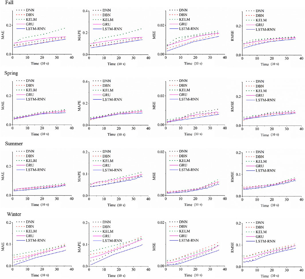
FIGURE 6. Performance of all measurement metrices with various prediction horizons in four seasons.
The prediction accuracy in four seasons varies. In the fall and spring season, the prediction errors are larger than the errors in the summer and winter season. This is due to a larger variability of the wind direction over short-term horizons. Hence, training specific prediction models in different seasons is necessary.
Table 1 provide the MAPE for different resolution data (i.e., 10, 20, 30 s) and different prediction horizons (i.e., 2, 5, 10 min, and 1 h) before the error correction. Obviously, the MAPE errors are smaller for the 10 s data than for 20 and 30 s. With the increase of the prediction horizon, the MAPEs increase. The LSTM-RNN algorithm has the smallest MAPE at all resolutions and all prediction horizons. Therefore, it is an effective algorithm for wind direction prediction at short-term horizons.
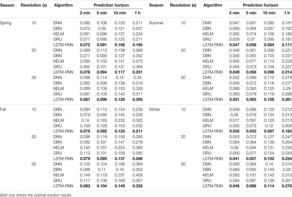
TABLE 1. Mape of the five algorithms for 2020 before error correction.
To correct the errors made by the ICEEMDAN modules, the ARIMA model has been developed to forecast the errors. In the second part of Figure 4, To illustrate this step, the forecasted errors using ARIMA versus the actual errors produced by LSTM-RNNs are visualized in Figure 7. It is obvious that the aggregated results from ARIMAs can represent the temporal trend of the forecasted errors produced from the first component of the proposed framework.
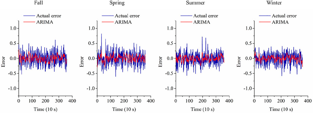
FIGURE 7. Actual error versus forecasted error by ARIMA models.
Table 2 provides the MAPE for different resolution data (i.e., 10, 20, 30 s) and different prediction horizons (i.e., 2, 5, 10 min, and 1 h) after the error correction. There exists significant performance for all algorithms tested with respect to the MAPE computed before and after error correction. It validates the effectiveness of implementing error correction in improving the forecasting accuracy of time-series dataset. Meanwhile, the LSTM produces the smallest errors which also demonstrates its superior performance in forecasting wind directions.
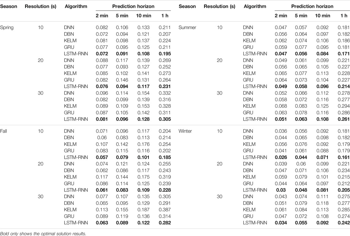
TABLE 2. Mape of the five algorithms for 2020 after error correction.
The experiments reported in Section “Short-term Predictions” have been conducted using the transformed wind direction data from four seasons. An inverse bilinear transformation, expressed in Eq. 2, is applied to transform the predicted transformed wind direction into the original angular range [0°, 360°]. The actual angular values versus the forecasted angular values by the proposed framework using ICEEMDAN and LSTM-RNN are presented in Figure 8. It can be seen that the majority of the forecasted values fall within a relatively small range with respect to the actual values. It demonstrates the proposed framework can sufficiently provide accurate forecasting performances.
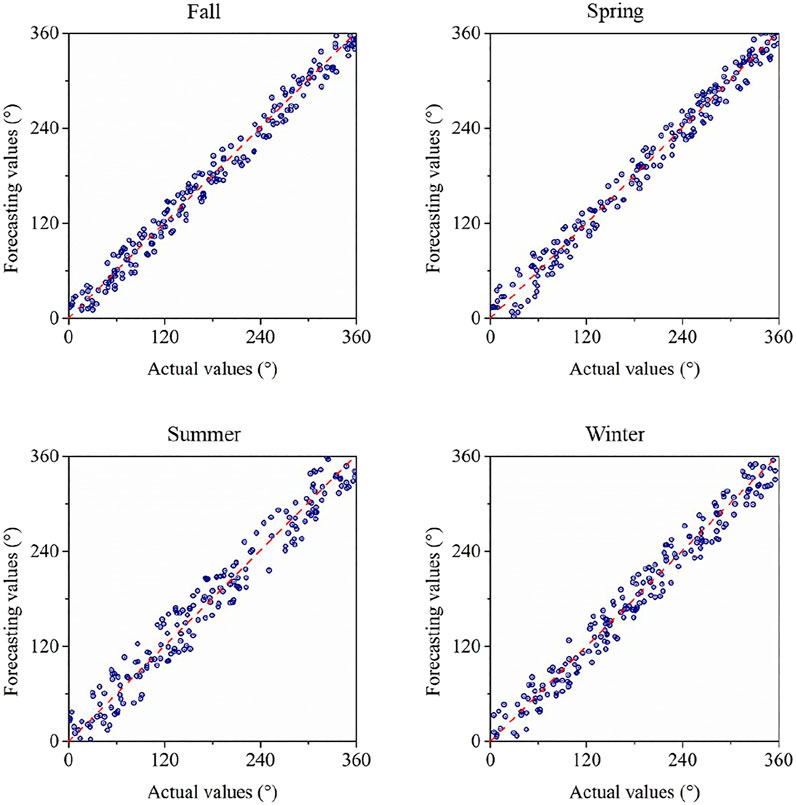
FIGURE 8. Actual angular values versus forecasting angular values.
In this section, performance of the ICEEMDAN framework integrated with the long-short-term memory recurrent neural network (LSTM-RNN) for prediction of wind direction at four seasons is discussed. The prediction error of the inverse transformed wind direction at 2, 5, 10 min, and 1 h horizons are presented in Table 3. The mean absolute error (MAE) and mean absolute percentage error (MAPE) of wind direction are smaller in the summer and winter.
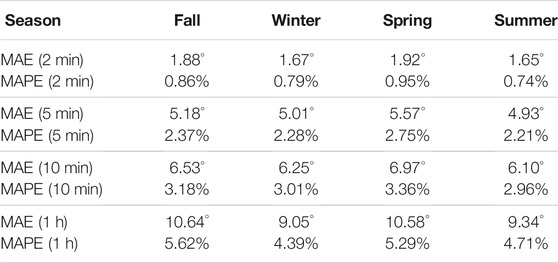
TABLE 3. Angular prediction error at four seasons.
The wind direction error shows less variability over short horizons. The changes of a nacelle position are usually made within 5 min and the prediction error should be under 3% (Ouyang et al., 2017). A control chart is applied to monitor the prediction error and facilitate changing the nacelle position. A control chart with lower and upper limits enables monitoring the yaw error. Any prediction error that exceeds the bound (i.e., 3%) may trigger a change of the nacelle position. The final forecasting errors in the angular perspectives are illustrated in Figure 9.

FIGURE 9. Wind rose of the prediction errors for the four seasons of interest in 2020.
The long-short-term memory recurrent neural network (LSTM-RNN) has been demonstrated to perform better than other algorithms. To validate the effectiveness and robustness of the LSTM-RNN, the data collected from another wind farm located in Shandong Province in the year 2020 has been used. The experiments are conducted following the similar training strategies as described in Section “Data Analysis”. The computational results are presented in Table 4.
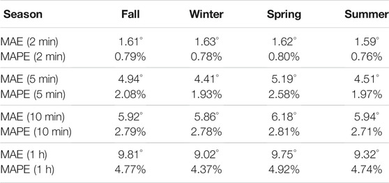
TABLE 4. Angular prediction error at four seasons.
The prediction error (see Table 4) in winter and summer seasons of 2020 from the wind farm in Shandong Province produced by the LSTM-RNN is similar to the one based on the 2020 data (see Table 3) in the wind farm in Inner Mongolia. More accurate performance has been observed in the fall and spring seasons with two prevailing wind directions. The favorable prediction error validates the effectiveness and robustness of the LSTM-RNN to predict the nacelle orientation.
A hybrid short-term forecasting framework to orient nacelle based on the predicted wind direction was presented. Industrial data collected from a wind farm in Inner Mongolia, China was utilized to train and validate the prediction models. A bilinear transformation was applied to transform the wind direction data from an angular variable into a continuous time-series. The forecasting framework was developed using ICEEMDAN integrated with LSTM-RNN. Also, the error corrections are implemented to improve the forecasting accuracy. The wind direction was predicted at short-term horizons, i.e., 2, 5, 10 min, and 1 h. Five algorithms, the deep neural network, deep belief network, kernel-based extreme learning machine, gated recurrent unit network, and long-short-term memory recurrent neural network were applied to predict wind direction at short-term horizons. The results of performance analysis of the five algorithms at four seasons were reported.
It was demonstrated that the long-short-term memory recurrent neural network outperformed the other four algorithms tested to predict wind direction. The results presented are of paramount importance in yaw control and can improve the efficiency of energy extraction process.
The raw data supporting the conclusions of this article will be made available by the authors, without undue reservation.
HL conceptualized the study, contributed to the study methodology, and wrote the original draft. JD contributed to the study methodology, data curation and investigation. PF contributed to data analysis and investigation. HL contributed to software and formal analysis. CP and DA contributed to investigation and writing-original draft. QC contributed to editing. All authors have read and agreed to the published version of the manuscript.
This research is supported by the “Miaozi project” of scientific and technological innovation in Sichuan Province, China (Grant No. 2021090), the National Key Research and Development Program of China (2018YFC1505105), the Opening fund of State Key Laboratory of Geohazard Prevention and Geoenvironment Protection (Chengdu University of Technology) (Grant No. SKLGP 2021K014), and the Project from Sichuan Mineral Resources Research Center (SCKCZY2021-YB009) the Project of remote sensing identification and monitoring of geological hazards in Sichuan province, CN (2020) (Grant No. 510201202076888).
Frontiers Media SA remains neutral with regard to jurisdictional claims in published maps and institutional affiliations.
The authors declare that the research was conducted in the absence of any commercial or financial relationships that could be construed as a potential conflict of interest.
All claims expressed in this article are solely those of the authors and do not necessarily represent those of their affiliated organizations, or those of the publisher, the editors and the reviewers. Any product that may be evaluated in this article, or claim that may be made by its manufacturer, is not guaranteed or endorsed by the publisher.
Amin, C. M., Sami, F. M., and Trzynadlowski, A. M. (2018). Wind Speed and Wind Direction Forecasting Using echo State Network with Nonlinear Functions. Renew. Energ. 131 (2), 879–889. doi:10.1016/j.renene.2018.07.060
Bilgili, M., Sahin, B., and Yasar, A. (2007). Application of Artificial Neural Networks for the Wind Speed Prediction of Target Station Using Reference Stations Data. Renew. Energ. 32 (14), 2350–2360. doi:10.1016/j.renene.2006.12.001
Castino, F., Festa, R., and Ratto, C. F. (1998). Stochastic Modelling of Wind Velocities Time Series. J. Wind Eng. Ind. Aerodynamics 74-76, 141–151. doi:10.1016/s0167-6105(98)00012-9
Cho, K., Van Merriënboer, B., Gulcehre, C., Bahdanau, D., Bougares, F., Schwenk, H., et al. (2014). Learning Phrase Representations Using RNN Encoder-Decoder for Statistical Machine Translation. doi:10.3115/v1/D14-1179
Colominas, M. A., Schlotthauer, G., and Torres, M. E. (2014). Improved Complete Ensemble EMD: A Suitable Tool for Biomedical Signal Processing.. Biomed. Signal Proce. Contr. 146, 19–29.
Davies, A. (1974). Bilinear Transformation of Polynomials. IEEE Trans. Circuits Syst. 21 (6), 792–794. doi:10.1109/tcs.1974.1083929
Duan, J., Zuo, H., Bai, Y., Duan, J., Chang, M., and Chen, B. (2021). Short-term Wind Speed Forecasting Using Recurrent Neural Networks with Error Correction. Energy 217, 119397. doi:10.1016/j.energy.2020.119397
Erdem, E., and Shi, J. (2011). ARMA Based Approaches for Forecasting the Tuple of Wind Speed and Direction. Appl. Energ. 88 (4), 1405–1414. doi:10.1016/j.apenergy.2010.10.031
Gers, F. A., Schraudolph, N. N., and Schmidhuber, J. (2003). Learning Precise Timing with Lstm Recurrent Networks. J. Machine Learn. Res. 3 (1), 115–143.
Groutage, F., Volfson, L., and Schneider, A. (2003). S-plane to Z-Plane Mapping Using a Simultaneous Equation Algorithm Based on the Bilinear Transformation. IEEE Trans. Automatic Control. 32 (7), 635–637. doi:10.1109/TAC.1987.1104664
Hochreiter, S., and Schmidhuber, J. (1997). Long Short-Term Memory. Neural Comput. 9 (8), 1735–1780. doi:10.1162/neco.1997.9.8.1735
Hu, Q., Zhang, R., and Zhou, Y. (2016). Transfer Learning for Short-Term Wind Speed Prediction with Deep Neural Networks. Renew. Energ. 85 (JAN), 83–95. doi:10.1016/j.renene.2015.06.034
Jury, E. (1973). Remarks on "The Mechanics of Bilinear Transformation". IEEE Trans. Audio Electroacoust. 21 (4), 380–382. doi:10.1109/tau.1973.1162485
Khosravi, A., Koury, R. N. N., Machado, L., and Pabon, J. J. G. (2018). Prediction of Wind Speed and Wind Direction Using Artificial Neural Network, Support Vector Regression and Adaptive Neuro-Fuzzy Inference System. Sustainable Energ. Tech. Assessments 25, 146–160. doi:10.1016/j.seta.2018.01.001
Kodama, K., and Burls, N. J. (2019). An Empirical Adjusted Enso Ocean Energetics Framework Based on Observational Wind Power in the Tropical pacific. Clim. Dyn. 53 (5), 3271–3288. doi:10.1007/s00382-019-04701-8
Kou, Z., Yang, F., Wu, J., and Li, T. (2020). Application of ICEEMDAN Energy Entropy and AFSA-SVM for Fault Diagnosis of Hoist Sheave Bearing. Entropy 22 (12), 1347. doi:10.3390/e22121347
Lecun, Y., Bengio, Y., and Hinton, G. (2015). Deep Learning. Nature 521 (7553), 436–444. doi:10.1038/nature14539
Lee, T.-H., White, H., and Granger, C. W. J. (1993). Testing for Neglected Nonlinearity in Time Series Models. J. Econom. 56 (3), 269–290. doi:10.1016/0304-4076(93)90122-l
Li, H., Xu, Q., He, Y., and Deng, J. (2018). Prediction of Landslide Displacement with an Ensemble-Based Extreme Learning Machine and Copula Models. Landslides 15 (10), 2047–2059. doi:10.1007/s10346-018-1020-2
Li, H., Xu, Q., He, Y., Fan, X., and Li, S. (2020). Modeling and Predicting Reservoir Landslide Displacement with Deep Belief Network and EWMA Control Charts: a Case Study in Three Gorges Reservoir. Landslides 17 (3), 693–707. doi:10.1007/s10346-019-01312-6
Liu, D., Niu, D., Wang, H., and Fan, L. (2014). Short-term Wind Speed Forecasting Using Wavelet Transform and Support Vector Machines Optimized by Genetic Algorithm. Renew. Energ. 62, 592–597. doi:10.1016/j.renene.2013.08.011
Liu, H., Shi, J., and Erdem, E. (2010). Prediction of Wind Speed Time Series Using Modified Taylor Kriging Method. Energy 35 (12), 4870–4879. doi:10.1016/j.energy.2010.09.001
Masseran, N., Razali, A. M., Ibrahim, K., and Latif, M. T. (2013). Fitting a mixture of von Mises distributions in order to model data on wind direction in Peninsular Malaysia. Energ. Convers. Manag. 72, 94–102. doi:10.1016/j.enconman.2012.11.025
Mcwilliams, B., and Sprevak, D. (1982). The Simulation of Hourly Wind Speed and Direction. Mathematics Comput. Simulation 24 (1), 54–59. doi:10.1016/0378-4754(82)90050-7
Mohandes, M. A., Halawani, T. O., Rehman, S., and Hussain, A. A. (2004). Support Vector Machines for Wind Speed Prediction. Renew. Energ. 29 (6), 939–947. doi:10.1016/j.renene.2003.11.009
Ouyang, T., He, Y., and Huang, H. (2018). Monitoring Wind Turbines' Unhealthy Status: a Data-Driven Approach. IEEE Trans. Emerging Top. Comput. Intelligence 3 (2), 163–172. doi:10.1109/TETCI.2018.2872036
Ouyang, T., He, Y., Li, H., Sun, Z., and Baek, S. (2019). Modeling and Forecasting Short-Term Power Load with Copula Model and Deep Belief Network. IEEE Trans. Emerg. Top. Comput. Intell. 3 (2), 127–136. doi:10.1109/tetci.2018.2880511
Ouyang, T., Kusiak, A., and He, Y. (2017). Predictive Model of Yaw Error in a Wind Turbine. Energy 123, 119–130. doi:10.1016/j.energy.2017.01.150
Pan, C., Yi, J., Yin, C., Yu, J., and Li, X. (2019). Joint 3D UAV Placement and Resource Allocation in Software-Defined Cellular Networks with Wireless Backhaul. IEEE Access 7, 104279–104293. doi:10.1109/access.2019.2927521
Peng, G., Si, C. A., Jc, B., and Di, C. (2020). Wind Direction Fluctuation Analysis for Wind Turbines. Renew. Energ. 162, 1026–1035. doi:10.1016/j.renene.2020.07.137
Rong, H., Gao, Y., Guan, L., Zhang, Q., Zhang, F., and Li, N. (2019). Gam-based Mooring Alignment for Sins Based on an Improved Ceemd Denoising Method. Sensors 19 (16), 3564. doi:10.3390/s19163564
Sak, H., Senior, A., and Beaufays, F. (2014). Long Short-Term Memory Based Recurrent Neural Network Architectures for Large Vocabulary Speech Recognition. arXiv preprint arXiv:1402.1128
Santhosh, M., Venkaiah, C., and Vinod Kumar, D. M. (2018). Ensemble Empirical Mode Decomposition Based Adaptive Wavelet Neural Network Method for Wind Speed Prediction. Energ. Convers. Manag. 168, 482–493. doi:10.1016/j.enconman.2018.04.099
Sun, Z., He, Y., Gritsenko, A., Lendasse, A., and Baek, S. (2020). Embedded Spectral Descriptors: Learning the point-wise Correspondence Metric via Siamese Neural Networks. J. Comput. Des. Eng. 7 (1), 18–29. doi:10.1093/jcde/qwaa003
Tagliaferri, F., Viola, I. M., and Flay, R. G. J. (2015). Wind Direction Forecasting with Artificial Neural Networks and Support Vector Machines. Ocean Eng. 97, 65–73. doi:10.1016/j.oceaneng.2014.12.026
Tang, Z., and Zhang, Z. (2019). The Multi-Objective Optimization of Combustion System Operations Based on Deep Data-Driven Models. Energy 182, 37–47. doi:10.1016/j.energy.2019.06.051
Tang, Z., Zhao, G., and Ouyang, T. (2021). Two-phase Deep Learning Model for Short-Term Wind Direction Forecasting. Renew. Energ. 173, 1005–1016. doi:10.1016/j.renene.2021.04.041
Wasynczuk, O., Man, D. T., and Sullivan, J. P. (1981). Dynamic Behavior of a Class of Wind Turbine Generators during Random Wind Fluctuations. IEEE Power Eng. Rev. PER-1 (6), 47–48. doi:10.1109/mper.1981.5511593
Xu, W., Yi, J., Dasgupta, S., Cai, J. F., Jacob, M., and Cho, M. (2018). “Sepration-free Super-resolution from Compressed Measurements Is Possible: an Orthonormal Atomic Norm Minimization Approach,” in 2018 IEEE International Symposium on Information Theory (ISIT) (IEEE), 76–80.
Yang, Z., and Wang, J. (2018). A Hybrid Forecasting Approach Applied in Wind Speed Forecasting Based on a Data Processing Strategy and an Optimized Artificial Intelligence Algorithm. Energy 160, 87–100. doi:10.1016/j.energy.2018.07.005
Yi, J., and Xu, W. (2020). Necessary and Sufficient Null Space Condition for Nuclear Norm Minimization in Low-Rank Matrix Recovery. IEEE Trans. Inform. Theor. 66 (10), 6597–6604. doi:10.1109/tit.2020.2990948
Zhang, W., Qu, Z., Zhang, K., Mao, W., Ma, Y., and Fan, X. (2017). A Combined Model Based on CEEMDAN and Modified Flower Pollination Algorithm for Wind Speed Forecasting. Energ. Convers. Manag. 136, 439–451. doi:10.1016/j.enconman.2017.01.022
Keywords: wind direction, bilinear transformation, ICEEMDAN, LSTM-RNN, error correction
Citation: Li H, Deng J, Feng P, Pu C, Arachchige DDK and Cheng Q (2021) Short-Term Nacelle Orientation Forecasting Using Bilinear Transformation and ICEEMDAN Framework. Front. Energy Res. 9:780928. doi: 10.3389/fenrg.2021.780928
Received: 22 September 2021; Accepted: 12 October 2021;
Published: 26 October 2021.
Edited by:
Tinghui Ouyang, National Institute of Advanced Industrial Science and Technology (AIST), JapanReviewed by:
Jirong Yi, The University of Iowa, United StatesCopyright © 2021 Li, Deng, Feng, Pu, Arachchige and Cheng. This is an open-access article distributed under the terms of the Creative Commons Attribution License (CC BY). The use, distribution or reproduction in other forums is permitted, provided the original author(s) and the copyright owner(s) are credited and that the original publication in this journal is cited, in accordance with accepted academic practice. No use, distribution or reproduction is permitted which does not comply with these terms.
*Correspondence: Jiahao Deng, amRlbmc1QGRlcGF1bC5lZHU=
Disclaimer: All claims expressed in this article are solely those of the authors and do not necessarily represent those of their affiliated organizations, or those of the publisher, the editors and the reviewers. Any product that may be evaluated in this article or claim that may be made by its manufacturer is not guaranteed or endorsed by the publisher.
Research integrity at Frontiers
Learn more about the work of our research integrity team to safeguard the quality of each article we publish.