 Bijay P Sharma
 T. Edward Yu
 Burton C. English
 Christopher N. Boyer2
- 1Institute for Sustainability, Energy and Environment, University of Illinois, Urbana-Champaign, IL, United States
- 2Department of Agricultural and Resource Economics, University of Tennessee, Knoxville, TN, United States
Sustainable aviation fuel (SAF) has been considered as a potential means to mitigate greenhouse gas (GHG) emissions from the aviation sector, which is projected to continuously expand. This study examines the impact of developing a SAF sector along with carbon credits on carbon equivalent emissions from aviation using a Stackelberg leader-follower model that accounts for economic interaction between SAF processor and feedstock producers. The modeling framework is applied to an ex-ante optimization of commercial scale SAF production for the Memphis International Airport from the switchgrass-based alcohol-to-jet pathway. Results suggest that supplying 136 million gallons of SAF to the Memphis International Airport annually could reduce 62.5% of GHG emissions compared to conventional jet fuel (CJF). Incorporating with carbon credits, SAF could lower GHG emissions by about 65% in total from displacing CJF and generate additional welfare gains ranging between $12 and $51 million annually compared to the case without carbon credits. In addition, sensitivity analysis suggests advancing SAF conversion rate from biomass could lower the SAF break-even considerably and enhance the competitiveness of SAF over CJF.
Introduction
There is mounting evidence that has documented the negative impacts of increasing cumulative anthropogenic greenhouse gas (GHG) emissions on human and environmental health [United States Environmental Protection Agency (EPA) 2017; Intergovernmental Panel on Climate Change Intergovernmental Panel on Climate Change (IPCC) 2014; Intergovernmental Panel on Climate Change (IPCC) 2018]. Lowering the atmospheric GHG concentration calls for actions that stabilize the atmospheric carbon content, which has been endorsed by numerous governments and private sectors across the world. One such action that has been a primary focus of researchers is lowering GHG emissions from the aviation sector (Grote et al., 2014). The International Air Transport Association (IATA) established goals of carbon neutral growth by 2020 and 50% GHG emissions reduction relative to the 2005 level by 2050 (IATA, 2015). Among various potential approaches to mitigate GHG emissions, utilizing renewable jet fuels (RJF) or sustainable aviation fuels (SAF) produced from agricultural and forestry residues, energy crops, or municipal wastes could have a crucial role in meeting the GHG emissions reduction goal (Fellet, 2016). As a “drop-in” fuel, SAF can be used in existing aircrafts without modifying engine designs or other engineering aspects (IATA, 2017).
The volume of SAF purchased by the U.S. aviation sector has increased from nearly zero in 2015 [U.S. Federal Aviation Administration (FAA), 2017] to about 4.5 million gallons in 2020 based on U.S. EPA’s Renewable Jet Fuel renewable identification numbers (RINs) data (Brown, 2021). In September 2021, the U.S. government announced a SAF Grand Challenge with the proposed goals to reach 3 billion gallons of SAF domestic production annually by 2030, and 35 billion gallons year−1 by 2050. Provision of tradable carbon credits could be a means to promote the use of SAF (Luo and Miller, 2013). Those carbon credits could be structured like RIN credits that are bought by registered blenders to ensure the compliance of a target or mandate. For example, the federal agency may issue GHG emission permits to the SAF processors and those permits can be traded in carbon market for credits.
Economic feasibility is considered as a key factor to expedite SAF production, thus studies related to SAF/RJF have primarily focused on the holistic economic assessment of various conversion technologies of SAF. Those studies estimated the break-even or minimum selling price (MSP) of SAF subject to conversion technologies and feedstock choices. Zhao et al. (2015) applied stochastic dominance rank study to identify the MSP for SAF at $3.11 gallon−1 of gasoline equivalent. Using stochastic dominance approach, Yao et al. (2017) found the mean break-even prices of $3.65 to 5.21 gallon−1 from various feedstock using the alcohol-to-jet (ATJ) pathway; whereas (Tao et al., 2017) estimated the MSP of $4.20 to $6.14 gallon−1 of SAF associated with the ethanol-to-jet (ETJ) upgrading technique. Bann et al. (2017) calculated the MSPs of Hydro-processed Esters and Fatty Acids (HEFA) and Fischer-Tropsch (FT) conversion pathways, and determined the MSP price ranging between $2.50 and 5.38 gallon−1 of SAF.
In addition to economic evaluations, a number of studies have examined the life cycle GHG emissions of SAF or RJF and indicated that replacing conventional jet fuel (CJF) with SAF/RJF could lower GHG emissions by 16–73% subject to feedstock choice and conversion pathways (Han et al., 2017). Specifically, Staples et al. (2018) indicated that SAF have the potential to reduce life cycle GHG emissions from aviation industry up to 68% in 2050 only if the policies were introduced to incentivize using bioenergy and waste feedstocks for SAF production over other alternative uses. The pathways of generating the SAF have substantial impacts on the GHG savings (O’Connell et al., 2019). Few studies have integrated carbon life cycle analysis (LCA) with economic analysis for SAF. Staples et al. (2014) calculated GHG footprint of SAF produced from Advanced Fermentation (AF) pathway and suggested RJF’s GHG emissions in the range of −27.0 to 89.8 gCO2e MJ−1 given the MSPs of $0.61 to $6.30 liter−1 ($2.31 to $23.85 gallon−1) from different feedstocks, compared to 90.0 gCO2e MJ−1 of CJF. Winchester et al. (2013) assessed the implicit subsidy required for SAF production from oilseed rotation crops via HEFA pathway, the cost of abating CO2 tonne−1 from the aviation from adopting SAF ranges between $50 and $400. Similarly, Winchester et al. (2015) evaluated the implicit subside for SAF produced via the AF pathway from perennial energy crops, and suggested the cost of abating CO2 equivalent could be from $42 to $652 tonne−1.
Despite the numerous studies on the economic assessment and LCA related to SAF, one key element generally neglected in these economic analyses of SAF is the potential interaction between feedstock producers and SAF processors. The biomass feedstock, such as perennial grass, cover crops, or forest residues, are not currently traded in the market. Therefore, it is important to incorporate feedstock producers’ decision process in allocating their scarce resources, such as land, when assessing the potential feasibility of SAF. Feedstock producers make decisions primarily based on their profit margins that account for a large portion of processors’ variable costs of SAF production (Agusdinata et al., 2011). As a result, the market price of SAF produced from a given feedstock-based conversion technology is a consequence to competition among the supply chain participants. Such interaction between the participants is influential to the optimization of bioethanol supply chains (Bai et al., 2012).
Another missing piece in the research on SAF production is the welfare analysis of SAF production and the probable policy mechanism. In order to achieve the determined target of the SAF Grand Challenge (3 billion gallons by 2030, 35 billion gallons by 2050) from the current level (∼4.5 million gallons in 2020), understanding the welfare implications to the related entities in the SAF supply chain could encourage more SAF production. In addition, how a GHG emissions policy or provision, such as carbon credits, may affect the optimization of SAF supply chain, net GHG emissions, and associated welfare for SAF processors and feedstock producers will provide important insights of policy mechanism on aviation GHG emissions reduction.
This study thus aims to contribute to the literature of SAF in two dimensions: first, the competitive interaction among the feedstock producers and the SAF processor is incorporated to determine the impacts of commercial-scale SAF production on farmland allocation, processing facility configuration, and GHG emissions using high resolution spatial data. Second, the impact of tradable carbon credits, a policy instrument for incentivizing the GHG emission reductions, on the welfare of the SAF processor and feedstock producers is assessed while addressing the economic interaction in the supply chain.
A Stackelberg leader-follower model is applied to capture the interaction of the SAF processor and feedstock producers and their location decision for biorefinery and feedstock draw area. As the follower, the feedstock producers are assumed to maximize their individual profits competing amongst each other in land use decision to fulfill the derived demand. The SAF processor, on the other hand, is the leader that maximizes its profit nesting the profit maximizing behavior of the individual feedstock producers. Under this circumstance, multiple decision makers from upstream to downstream of the supply chain are involved in the decisions of resource (farmland) allocation and site selection. Such sequential decision process can be formulated as a bi-level optimization problem (Lim and Ouyang, 2016), which indicates that the leader (SAF processor) considers the follower’s (feedstock producer) optimization outcome when optimizing its goals (Sinha et al., 2018).
The modeling framework is applied to an ex-ante optimization of supplying switchgrass as feedstock for SAF production to meet 50% of the aviation fuel use in the Memphis International Airport (MEM). Switchgrass is selected as the feedstock given its suitability to the soil and weather condition in the southeastern region (Wright and Turhollow, 2010). Given the selected biomass feedstock, the ATJ pathway is selected for the analysis since it is one of the technical feasible technologies to convert biomass to SAF (Yao et al., 2017). The findings from this study should provide researchers, the industry, and policy makers more insights of the potential economic and environmental impacts of developing a commercial scale SAF for the aviation industry. The modeling framework can be applied to alternative feedstock and the associated SAF pathways in different regions.
Analytical Methods
A supply chain framework entailing game-theoretic competition between the feedstock producers and the SAF processor is implemented to analyze the economic and environmental metrics of the SAF supply chain. Following (Bai et al., 2012), the interactive decision process is modeled as a Stackelberg leader-follower game with farmland use and facility location decisions. Illustrated in Figure 1, the SAF processor (leader) select farmers for contracts based on the types of lands with a predetermined payment under the situation with carbon credit (the Baseline) and without the credit (alternative scenarios), and farmers (follower) choose to accept or decline the offer price for converting their current land use to supply feedstock. Farmers compete for the contracts without cooperative arrangements. Since there is no well-established market for large volume switchgrass transaction, land use changes are the primary decisions that go into the profit maximization problem of the feedstock producers. The “take it or leave it” feedstock price is exogenously determined by the processor based on the quantity of SAF to be produced. Since the SAF price is exogenously determined as a contractual agreement between the processor and the airlines rather than a market clearing mechanism, the processor’s profit maximization is essentially a cost minimization problem.
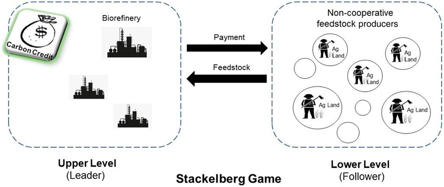
FIGURE 1. The Stackelberg leader-follower game of the SAF feedstock supply chain. Note: Figure is adapted from Figure 2 in Yao et al. (2019).
The model assumes that the SAF processor determines the break-even price for the SAF before accepting the airlines’ offered price leading to an offtake agreement1. The SAF processor then decides the feedstock price and offers an identical price to all feedstock producers in the region. An individual feedstock producer’s decision to accept the offered price for producing biomass feedstock is determined by whether the offered price meets the producer’s minimal profits expectation or not. Essentially, the processor chooses a processing capacity for the potential plant with its spatial configuration along with a price offered to the feedstock producers that minimizes its feedstock procurement and the SAF processing costs. Finally, a premium above the break-even price obtained from the processor’s bi-level optimization is assumed as the contract price between airlines and the SAF processor to satisfy the profit of the processor.
Feedstock Producer’s Profit Maximization
Feedstock producers decide on biomass supply quantities to maximize their profits based on the exogenous feedstock price offered from the processing facility subject to land availability and SAF demand. Feedstock producers’ objective is generalized as:
where
The first summation term in Eq. 1 presents the revenues from feedstock supply subtracting transportation costs during harvest season, while the second summation term represents the revenues after deducting feedstock transportation and storage costs during the off-harvest season. The third component sums up annualized feedstock establishment, harvest, maintenance, and the opportunity costs of land use change. Opportunity cost is defined as either net return from existing land use or land rent, whichever is higher (Yu et al., 2016), given by:
where
The profit maximization problem is subject to certain constraints presented in Eqs. 2–8 below. Eq. 2 limits feedstock production area to the available agricultural land. Eq. 3 assures that total harvested biomass equals the total biomass production. Eq. 4 models the competitive relationship between the individual feedstock producers and assures that biomass supplied by profit maximizing feedstock producers together does not exceed the production capacity of the processing facility. Eqs 5, 6 are mass balance/flow constraints. Eqs 7, 8 are the non-negativity constraints imposed on the continuous decision variables.
where
Processor’s Bi-level Optimization Problem
The SAF processor also aims to maximize profit assuming the final SAF price is a contract between the processor and the airlines once the processor determines its break-even level and its profit margins. Thus, the processor needs to decide on biomass procurement price and the configuration of facilities to minimize its costs as its break-even level subject to the anticipated optimal behavior of the feedstock producers. The processor’s profit maximization objective is thus converted to a cost minimization objective as:
where
Eqs 10–15 below define the constraints imposed on the cost minimization problem. Eq. 10 ensures that the amount of biomass transported during each season is all converted into SAF by processing facility. Eq. 11 guarantees SAF sent to airport in each season meets the seasonal demand of SAF by the airlines. Eq. 12 limits the number of processing plants at each site. Eqs 13, 14 denote the domains of the binary and continuous decision variables. Eq. 15 assures that profit of individual feedstock producers to be at least
Solution Approach to Bi-level Optimization
Since the profit maximization problem of the feedstock producers (lower-level problem) is linear, the typical approach to solving the bi-level optimization is to convert it into a single-level optimization by replacing the original constraints of the lower-level including the objective function by its corresponding Karush-Kuhn-Tucker (KKT) conditions. The KKT conditions guarantee the objective function and all the constraints corresponding to individual feedstock producer’s profit maximization problem are satisfied. The KKT transformation is a non-convex non-linear problem which is often difficult to solve (Gümüş and Floudas, 2005). These KKT constraints are thus reformulated as disjunctions with the introduction of slack variables, and converted into mixed-integer constraints using the Big-M and binary variables (Gümüş and Floudas, 2005). The resulting problem then becomes linear and is solved using the CPLEX solver of the General Algebraic Modeling System (GAMS) 24.2 (Rosenthal, 2008).
GHG Emissions, SAF Co-products and RIN Credits
The LCA-based GHG emissions from SAF2 is estimated to evaluate the environmental impact of SAF. The estimated total supply-chain GHG emissions include GHG emissions from land use change into switchgrass; energy use emissions from switchgrass production, harvest, and storage; emissions from energy use during transportation of biomass and SAF; and the emissions related with feedstock grinding and conversion.
As the ATJ pathway produces other hydrocarbon fuels as co-products in addition to the SAF, estimation of LCA-based GHG emissions for the main-product should account for the contribution of its co-products (Wang et al., 2011). GHG emissions from the co-products are calculated using an allocation method based on their approximately equal energy contents (Han et al., 2017). In addition, the revenue generated from the co-products by displacing the fossil fuels is estimated using the displacement method at the market prices of fossil fuels. In particular, the environmental benefit of SAF and its co-products is assessed by estimating changes in GHG emissions between the energy products from the ATJ-pathway (SAF, cellulosic-diesel, and cellulosic-gasoline) and the displaced fossil fuels (CJF, diesel, and gasoline).
The Renewable Fuel Standard program established in the Energy Policy Act of 2005 is a market-based compliance system that utilizes RIN credits as a mechanism to trace if biofuel refiners or terminal operators produce the mandated level of biofuels under the Energy Act. Two different RIN credits for cellulosic biofuel based on average price for 2016 (2016-A), and 2017 (2017-A) are considered to examine its impacts on economic feasibility of SAF. The impact of revenues from ATJ co-products as well RIN credits is exogenous since they are taken as additional economic incentives for supporting SAF production. Thus, RIN credits, revenues, and GHG emission reductions from co-products are included in estimating the cost, environmental, and welfare impacts of SAF.
Welfare Analysis of the SAF Sector
Given the price assumptions used in satisfying the economic objectives of the supply-chain participants, surpluses for feedstock producers (
where
Carbon Credits Analysis
For a processor, the choice for the processing facility location and the contracted feedstock producers could vary considerably whether carbon credits are available or not at the investment stage. The presence of tradable carbon credits incentivizes the SAF processor to reduce the total field-to-wake GHG emissions since the total value of carbon credits is proportional to the difference in energy equivalent well-to-wake (fuel extraction to combustion) GHG emissions from CJF and field-to-wake GHG emissions from SAF. The reduction in GHG emissions for the SAF processor is achieved either through contracting feedstock producers for crop land conversion to switchgrass because of net carbon sequestration or by reducing feedstock and SAF transportation GHG emissions through optimal facility location. To estimate the economic, environmental and welfare implication of the hypothetical carbon credits on the SAF supply-chain, the system is defined in Eqs. 1–15 as the Baseline in which SAF processor and feedstock producers make their decisions without carbon credits. In contrast, under the alternative scenarios of having carbon credit, the augmented objective function of SAF processor in Eq. 9 is defined as follows:
where
Three different carbon credit scenarios corresponding to historical low and high carbon prices in the California Cap-and-Trade program (CalCaT-L and CalCaT-H, respectively), and historical high carbon price in the European Union Emission Trading System (EUETS-H) are used to evaluate the impact of potential carbon markets in GHG emissions reduction and supply-chain welfare. These scenarios are selected to reflect the ranges of the U.S. as well as the global carbon prices in the emission trading market. In each scenario, a share of the total carbon credits per gallon of SAF (
The leader-follower nature merits the processor in a way that impacts the optimal land use decisions of the feedstock producers through its facility location decisions under carbon credits. The processor is able to simultaneously lower the break-even SAF price and GHG emissions since the total carbon credits is proportional to the GHG emissions reduction compared to equivalent CJF. This decision process changes net welfare primarily through changes in the surpluses for feedstock producers, the processor, and the airlines as follows:
where
Data
The data used for cellulosic ATJ conversion pathway is categorized into two groups: feedstock-based ethanol production data, and the data on potential conversion technology of ethanol to SAF. The parameters used to calculate costs and GHG emissions of feedstock-based ethanol production are from (Yu et al., 2016); whereas the parameters used for calculating costs, yields including co-products, and GHG emissions of ethanol-to-SAF conversion are primarily based on recent techno-economic analysis of feedstock-based ATJ or ETJ conversion pathways (Elgowainy et al., 2012; Han et al., 2017; Tao et al., 2017; Yao et al., 2017). The ethanol-to-SAF conversion parameters are augmented with relevant feedstock-based ethanol production data in estimating the feedstock-to-SAF conversion parameters.
Data from switchgrass field trials between 2006 and 2011 at west Tennessee (Boyer et al., 2012; Boyer et al., 2013) is used to simulate feedstock yields across 5 sq. mile spatial units on existing agricultural lands. Mean yields obtained from normally distributed simulations are matched to the number of potential feedstock producers supplying feedstock. Spatial yield variation is determined following the simulated spatial variation in switchgrass yields in the region (Jager et al., 2010). A total of 18 industrial parks are identified as candidates for establishing processing facilities. Each location can have at most one facility with the capacity of either 50 million gallons year−1 (MGY) or 100 MGY. Similarly, a total of 1936 hexagon-shaped spatial units (5 mile2 per unit) are taken as potential feedstock producers opting to cultivate switchgrass replacing current crops. An annual SAF demand of 136 million gallons for the MEM is assumed which replaces one-third of the total jet fuel consumption for flights departing from the MEM airport in 20164. The price feedstock producers received at the processing facility gate in the study region is $75 ton−1 derived from the estimated average plant gate cost of switchgrass delivered to an ethanol plant in west Tennessee in Yu et al. (2016).
Table 1 presents key conversion parameters used in the analysis including co-products i.e. cellulosic-gasoline and cellulosic-diesel. Conversion cost and GHG emissions in the table refer to the parameters associated with feedstock-to-SAF conversion excluding feedstock grinding. The cost and GHG emission parameters on feedstock grinding are taken into account separately based on (Yu et al., 2016). The LCA-based GHG emissions of displaced conventional energy products (fossil fuels) are shown in Table 2. The market prices of fossil fuels displaced by corresponding ATJ products are also included in Table 2. Table 3 shows the levels of RIN credits5 used and carbon credits considered for specific carbon credit scenarios. The social cost of carbon, $33.70 tonCO2e−1, is adapted from (Nordhaus, 2017).
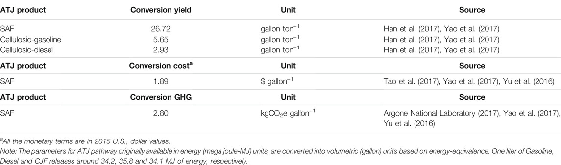
TABLE 1. Parametric assumptions for cellulosic alcohol-to-jet (ATJ) conversion pathway.
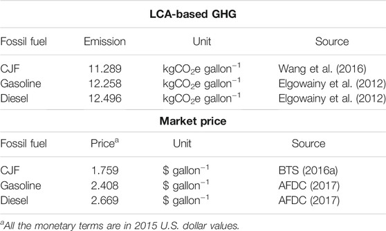
TABLE 2. Parameters on energy-equivalent substitutes to ATJ products.
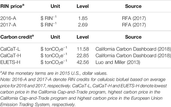
TABLE 3. RIN credits and parameters for carbon credit scenarios.
Results and Discussion
The Baseline Solutions of the Stackelberg Model
Supply-Chain Economic and GHG Emissions Outputs
Under the Baseline, the overall cost accrued by the SAF processor from the optimal game-theoretic model is $1,155 million year−1, while the aggregate profit of feedstock producers is $16.88 million. The optimal location of processing facility and the contracted individual feedstock producers are shown in Figure 2. An important factor in producers’ decision on converting their land to a new operation is the opportunity cost of land use change. Selection of land for food crops had higher opportunity costs than pasture land. Additionally, spatial variation in switchgrass yields across west Tennessee creates comparative advantage to some of the potential feedstock producers. A total of 657,000 acres of farmland are selected for feedstock cultivation with more than 58% converting from pasture land. Crop land use changes occur with soybean and corn acreages shifting to switchgrass production.
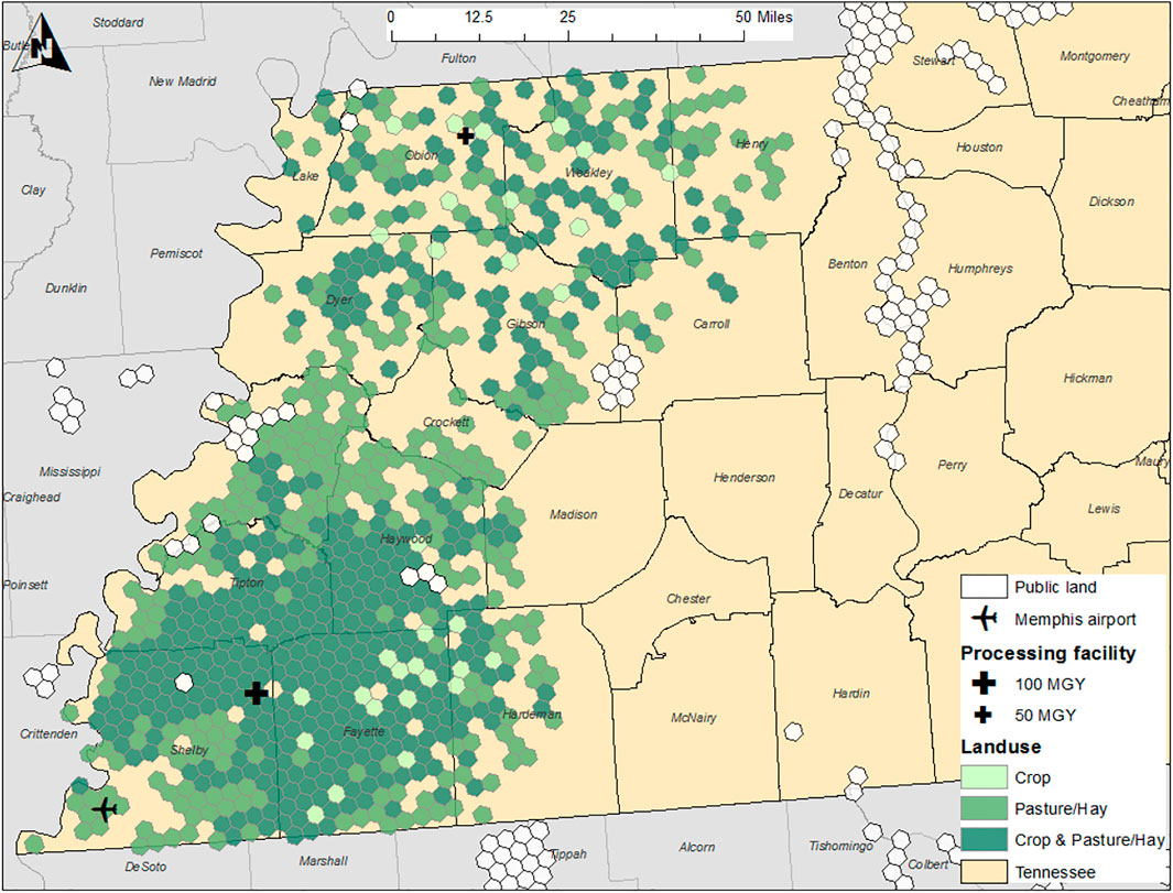
FIGURE 2. Optimal land use and facility locations under the Baseline.
The processor’s facility configuration decisions are influenced by the spatial distribution of the potential feedstock producers, their opportunity costs of supplying feedstock, and the spatial yield variability. The processor decides to locate a larger processing facility (100 MGY capacity) at a site surrounded by feedstock producers farming agricultural lands with lower opportunity costs. On the other hand, feedstock producers with higher yields are pivotal in determining the location for the 50 MGY facility simultaneously securing their profit margins.
The margin over the opportunity cost gained by feedstock producers from supplying feedstock is shown in the Figure 3. Most of the feedstock producing areas (more than 57%) received a margin ranging from 10 to 47% over their opportunity cost of converting the land, whereas a few feedstock producing areas obtained substantial margins of up to 658%. The observed gains are primarily dictated by the types of land used for feedstock cultivation. In general, the margin is higher for feedstock producers converting pasture land. Because of the higher opportunity costs of cropland, less margin is acquired in areas with significantly more cropland when compared to pastureland, resulting conversion of either crop land alone or a mix of the pasture and crop land.
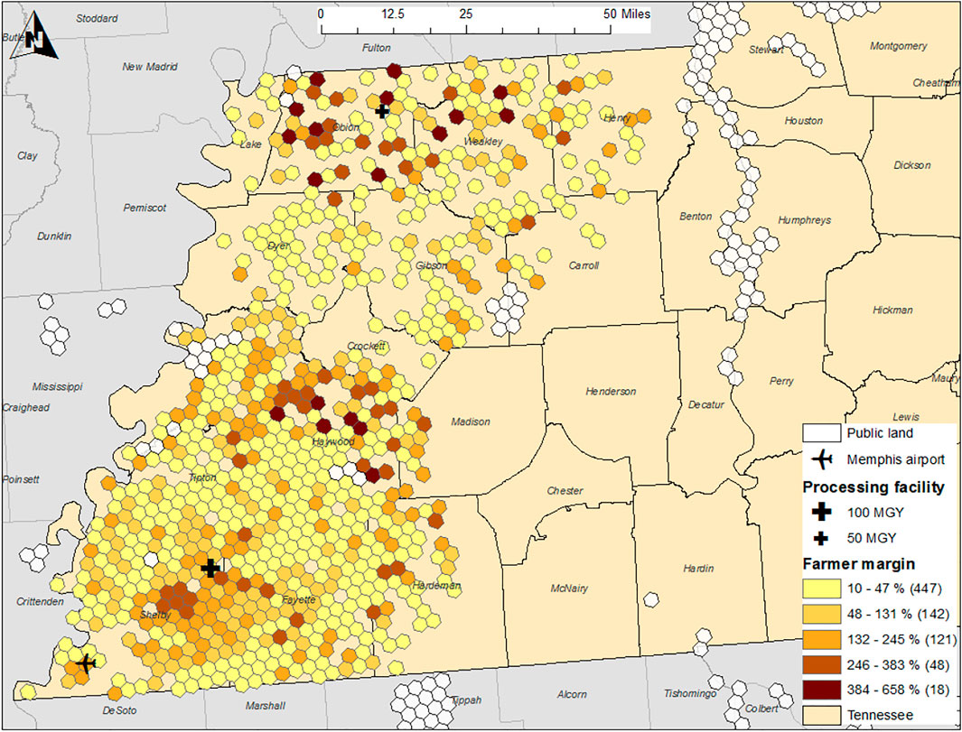
FIGURE 3. Margins of individual feedstock producers under the Baseline. Note: Number in the parenthesis refers the amount of feedstock producers.
The annualized costs and GHG emissions of each operation in the bi-level supply-chain optimization for the Baseline are summarized in Table 4. The largest component of the processor’s cost is related to SAF conversion, around $515 million year−1. Similarly, feedstock procurement (approximately $382 million) consists of a sizeable portion of the processor’s cost. With a conversion factor of 26.72 gallons ton−1, a total of 5.09 million tons of feedstock are procured for fulfilling the SAF demand at the MEM airport. Feedstock harvest cost of nearly $114 million are the highest costs incurred in aggregate, followed by feedstock transportation cost of around $107 million.
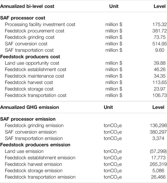
TABLE 4. Annualized variables for the Baseline.
The conversion process produces the highest GHG emissions, above 380,000 tons of CO2e with feedstock harvest producing around 265,000 tons of CO2e emissions annually. Land use change results in sequestration of around 57,000 tons of CO2e emissions, primarily through crop lands conversion to switchgrass because of net carbon sequestration in the soil. More than 777,000 tons year−1 of CO2e emissions are generated from this switchgrass-based SAF supply chain. The total LCA-based GHG emission reduction through displacement of the fossil fuels with the ATJ-pathway is 62.5% under the Baseline, which lies within the range of 16–80% estimated in Han et al. (2017) for various feedstock conversion pathways.
Supply-Chain Welfare Analysis
In this study, the producer surpluses for feedstock producers (denoted as PS-FS) are equal to the total feedstock producer profit, while and the SAF processor surpluses (denoted as PS-SAF) and the processor’s profit. The feedstock producers’ economic surplus is about $16.9 million, while the SAF processor secures a surplus of $13.6 million. The consumer surpluses for the SAF (denoted by CS-SAF) are -$256.8 million and $158 thousand with 2016-A and 2017-A RIN credits, respectively, for the Baseline. Internalized environmental costs of aviation GHG emissions of around $26.2 million result in net supply-chain welfares -- around -$252.5 million and $4.44 million with 2016-A and 2017-A RIN credits, respectively, for the Baseline.
The large negative values in the estimated social welfare is mainly related to prohibitively expensive production and processing costs of switchgrass-based SAF. This is in line with the prior studies indicating cellulosic biofuel mandates with the blending credits may have large negative welfare estimates because of heightened production costs and burden to taxpayers (Chen et al., 2011). Even though there are no explicit SAF mandates and subsidies in place, a recent analysis of SAF produced from Camelina sativa shows that a combination of 9% subsidy on the SAF and 9% tax on the CJF would make it at least revenue neutral to the government otherwise society would have to bear a large cost (Reimer and Zheng, 2017).
Comparison Between the Baseline and Carbon Credit Scenarios
Changes in Optimal Solutions for the Bi-level Objectives
Under the scenarios of available carbon credits, the SAF processor decides on facility locations and the contracted feedstock producers in such a way that reduces the total field-to-wake GHG emissions through contracting feedstock producers converting crop lands for switchgrass production or siting facility that reduced feedstock and SAF transportation GHG emissions (see Supplementary Figures SA1–A3 for the CalCaT-L, CalCaT-H, and EUETS-H scenarios, respectively, in the Appendix). The changes in the annualized costs of related operations in the supply chain from introducing carbon credits is summarized in Table 5. Compared to the Baseline, total annual feedstock producer profit declines by $5.88, $5.90, and $10.45 million for the CalCaT-L, CalCaT-H, and EUETS-H scenarios, respectively, as the opportunity costs of land use increased. The crop land use increases by around 98,000 to 151,000 acres for the three scenarios. Meanwhile, there are subsequent reductions in pasture land conversion under all three scenarios.
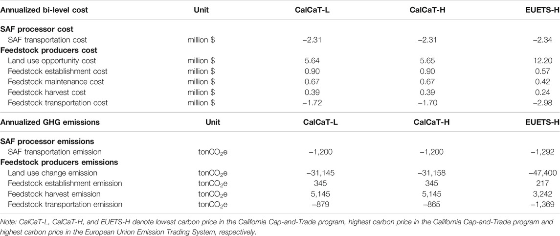
TABLE 5. Changes in annualized variables for carbon credit scenarios compared to the Baseline.
In addition, the processor locates the facility closer to the MEM airport to reduce SAF transportation GHG emissions in response to carbon credits (see Figs. A1, A2, and A3 for the CalCaT-L, CalCaT-H, and EUETS-H scenarios, respectively, in the Appendix). As a result, the processor’s transportation cost also declines. The highest carbon credit scenario, i.e. EUETS-H, triggers major land use changes and facility location, increasing the objective values compared to the no carbon credit case. Similarly, increased cropland use in response to proximity of the facility reduced the feedstock transportation costs by $1.72, $1.70, and $2.98 million for the CalCaT-L, CalCaT-H, and EUETS-H scenarios, respectively.
Total annual GHG emissions in the SAF supply chains are reduced between 27.7 to more than 46.6 thousand tonCO2e under the three carbon credit scenarios compared to the Baseline. As expected, the highest carbon credits (EUETS-H scenario) creates the most impact on GHG emissions reduction from the Baseline, while the changes in GHG emissions for the CalCaT-L and CalCaT-H scenarios are similar. As shown in Table 5, major GHG emission reductions from all the carbon credit scenarios are associated with land use change. Reductions in GHG emissions associated with feedstock and SAF transportation are relatively small. With carbon credits, the total GHG emission reductions from using SAF and its co-products range between 64 and 65% among all three scenarios when compared to the displaced CJF and other fuel products.
Change in the Supply Chain Welfare
The changes in net welfare for different carbon credit scenarios against the Baseline is illustrated in Figure 4. A subsequent decrease in the SAF processor’s break-even price incurs given higher carbon credits. The margin under carbon credits improves the surplus for the SAF processor. Similarly, the surplus for the SAF consumers, i.e., airlines, increases as the SAF price at each carbon credit scenario is lower than the Baseline. However, the surplus for the feedstock producers, i.e. feedstock producers, reduces due to more high opportunity cost crop lands converted for feedstock production driven by the carbon credits acquired by the SAF processor.
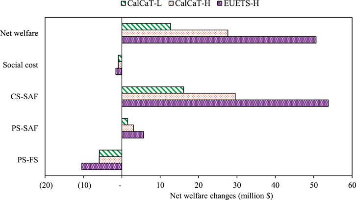
FIGURE 4. Changes in net welfare for carbon credit scenarios against the Baseline. Note: PS-FS, PS-SAF and CS-SAF denote surplus for feedstock producers, surplus for SAF processor and surplus for SAF consumers, respectively. CalCaT-L, CalCaT-H and EUETS-H denote lowest carbon price in the California Cap-and-Trade program, highest carbon price in the California Cap-and-Trade program and highest carbon price in the European Union Emission Trading System, respectively.
Subsequent abatements in the GHG emissions from carbon credits reduce the social cost of emissions compared to the Baseline in each carbon credit scenario. The net welfare increases across all carbon credit scenarios because of the consumer surplus increase toward the airlines. Under the minimum carbon credit (CalCaT-L scenario) scenario,. the SAF processor’s surplus increases by $1.53 million and economic surplus of airlines increases by $16.12 million. However, feedstock producers’ surplus decreases by $5.88 million due to the selection of higher productive cropland (with higher opportunity cost) that can store more soil carbons after being converted to switchgrass. With $935,000 reduction in the internalized costs of field-to-wake GHG emissions, the net welfare increases by $12.71 for the CalCaT-L scenario compared to the Baseline. Similarly, the net welfare increases by $27.61 and 50.62 million for the CalCaT-H and EUETS-H scenarios, respectively, mainly due to increments in the airlines’ surpluses.
In this study, the benefit of a tradable carbon credit is reaped by the SAF processor only even though the reduction in GHG emissions is based on field-to-wake approach. This is because it is assumed that the processor as a leader can reduce field-to-wake GHG emissions indirectly by contracting feedstock producers that convert crop land due to net carbon sequestration, or directly by reducing feedstock and SAF transportation GHG emissions through optimal facility location. If the portion of the carbon credit is allocated to the feedstock producers for soil carbon sequestration, the competition for feedstock and related land use decisions could be different.
Economic Feasibility and GHG Emission Abatement Cost
The inclusion of cellulosic RIN credits has a substantial impact in lowering the break-even SAF price as well as the cost of aviation emission abatement. Figure 5 depicts the break-even prices6 for the SAF considering two levels of cellulosic RIN credits (2016-A and 2017-A) along with revenues from the co-products in the Baseline and three carbon credit scenarios. With the 2017-A RIN credit ($2.69 RIN−1), the feedstock processor’s break-even for the SAF ($1.65 gallon−1) is lower than the market price of the CJF ($1.76 gallon−1) regardless of the availability of carbon credits. The SAF remains price-competitive with 2017-A RIN credits after implementing the markup of $0.10 gallon−1. If the RIN credit is at the level 2016-A ($1.85 RIN−1), the SAF is not economic competitive with CJF in both the Baseline and the carbon credit scenarios.
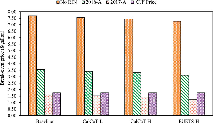
FIGURE 5. SAF break-even prices with RIN credits and revenues of co-products. Note: 2016-A and 2017-A denote RIN credits for cellulosic biofuel based on average price for 2016 and 2017, respectively. CalCaT-L, CalCaT-H and EUETS-H denote lowest carbon price in the California Cap-and-Trade program, highest carbon price in the California Cap-and-Trade program and highest carbon price in the European Union Emission Trading System, respectively.
Cost associated with the LCA-based GHG emissions reduction using SAF and its co-products from the ATJ-pathway varies across the Baseline and the carbon credit scenarios. With 2017-A RIN credit, the SAF price ($1.75 gallon−1) is lower than the market price of the CJF even without the carbon credits, thus no additional cost of GHG emission abatement. However, if the RIN credit remained at 2016-A level, the implicit subsidy from the airlines to the processor is $1.89 gallon−1 for the Baseline, which decreases to $1.77, $1.67, and $1.49 gallon−1 for the CalCaT-L, CalCaT-H, and EUETS-H scenarios, respectively. Given the 2016-A RIN credit, the implicit cost of abatement for the airlines is $198 tonCO2e−1 for the case of no carbon credits. The estimated abatement cost is within the range of other estimates for SAF produced from oilseed rotation crops and perennial energy crops (Winchester et al., 2013; Winchester et al., 2015). The abatement cost estimates further decreases to $182, $172, and $151 tonCO2e−1 for the CalCaT-L, CalCaT-H, and EUETS-H scenarios, respectively.
To sum up, the findings suggest that the evaluated carbon credits are found influential in reducing aviation GHG emissions while simultaneously improving net welfare of SAF sector. However, the level of RIN credits largely determines the economic feasibility of SAF.
Sensitivity Analysis
As land use competition is critical to the objective of feedstock producers and the SAF processors in this bi-level optimization model (Bai et al., 2012), factors influencing land use choice are further evaluated in the sensitivity analysis. The first key parameter is feedstock procurement price given its directly impact on farmers’ profit, and consequently influence on the location of feedstock supply and the location of biorefineries. The SAF conversion rate is another crucial factor. It determines the required feedstock quantity and resulting land use competition for feedstock supply, and the profit of farmers and SAF producers.
Feedstock Procurement Price Sensitivity Analysis
Two feedstock procurement prices are evaluated in the sensitivity analysis: $60 ton−1 (15% below the baseline feedstock price of $75 ton−1) and $90 ton−1 (10% above the baseline feedstock price) in presence of cellulosic RIN credits. With a feedstock price of $60 ton−1, there would not be sufficient number of feedstock producers to supply required feedstock quantity for the SAF demand at the MEM airport. Thus, SAF processor would not operate when offering switchgrass producers $60 ton−1.
Assuming the feedstock price is offered at $90 ton−1, the feedstock processor’s break-even for SAF is $4.07 gallon−1 with 2016-A RIN credits. With the 2017-A RIN credits, the SAF processor’s break-even price is $2.18 gallon−1, making SAF economically infeasible at both RIN credit levels. Considering a $0.10 gallon−1 markup for the SAF processor, the implicit subsidy from the airlines to the processor ranges from $2.03 to $2.41 gallon−1 in the Baseline and the carbon credit scenarios cases under the provision of 2016-A RIN credits (Table 6). Equivalently, the airline’s implicit abatement cost is $251 tonCO2e−1 for the Baseline, which decreases to $232, $216, and $204 tonCO2e−1 for the CalCaT-L, CalCaT-H, and EUETS-H scenarios, respectively. Similarly, under the availability of 2017-A RIN credits, the implicit GHG emissions abatement cost for the airlines is $54 tonCO2e−1 for the Baseline case and decreases to $45, $36, and $15 tonCO2e−1 for the CalCaT-L, CalCaT-H, and EUETS-H scenarios, respectively.
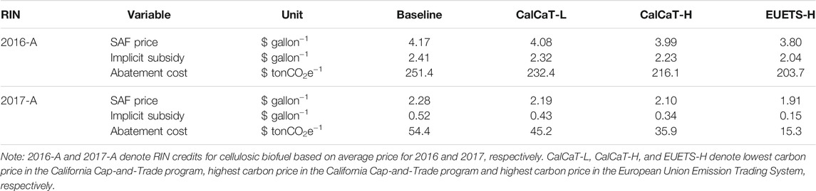
TABLE 6. GHG emission abatement costs with feedstock price at $90 ton−1.
With the assumed feedstock price of $90 ton−1, the aggregate net farm income increases and the economic surplus for the feedstock producers is $59.5 million. Without carbon credits, social cost of aviation GHG emissions is around $26.0 million and leading to a net supply-chain welfare of approximately -$280.6 million and -$23.7 million with 2016-A and 2017-A RIN credits, respectively. Under the availability of CalCaT-L carbon credits, the SAF processor’s surplus increases by $1.6 million, and the airlines’ economic surplus increases by $12 million, while feedstock producers’ surplus decreases by $2.7 million compared to the Baseline. Thus, the net supply-chain welfare for the CalCaT-L scenario increases by $12.8 with a reduction of $1.9 million in the internalized costs of aviation GHG emissions relative to the Baseline. Similarly, the net supply-chain welfare increases by $24.3 and 51.7 million for the CalCaT-H and EUETS-H scenarios, respectively, compared to the Baseline.
Displacing CJF with the ATJ-pathway SAF produced from switchgrass at a price of $90 ton−1 reduces the total LCA-based GHG emissions by 63% under the Baseline. With carbon credits, the total GHG emission reductions from SAF and its co-products reach to 65.5–68% for the three carbon credits scenarios compared to utilizing CJF in the aviation sector.
SAF Conversion Rate Sensitivity Analysis
Sensitivity of SAF conversion rate on economic feasibility of SAF production and associated GHG emission abatement cost is examined with two levels of conversion rate: 24.05 gallons ton−1 (10% below the Baseline conversion rate at 26.72 gallons ton−1) and 29.40 gallons ton−1 (10% above the Baseline rate) in presence of cellulosic RIN credits. With a conversion rate of 24.05 gallons ton−1, the demand for feedstock increases but there would not be sufficient feedstock producers to supply required feedstock quantity for the SAF demand. Therefore, SAF processor would not be able to operate given the lower conversion rate.
If the conversion rate improves to 29.40 gallons ton−1, the break-even for SAF decreases to $3.25 gallon−1 with 2016-A RIN credits. With a $0.10 gallon−1 markup for the SAF processor, the implicit subsidy from the airlines to the processor is between $1.35 and $1.59 gallon−1 in the Baseline and the carbon credit cases under the provision of 2016-A RIN credits (Table 7). Equivalently, the implicit GHG emissions abatement cost for the airlines is $165 tonCO2e−1 under the Baseline, which decreases to $152, $144, and $134 tonCO2e−1 for the CalCaT-L, CalCaT-H, and EUETS-H scenarios, respectively. At the higher conversion rate (29.40 gallons ton−1) and assuming the 2017-A RIN credits, SAF becomes price-competitive to the CJF ($1.36 vs. $1.75 gallon−1) even without the carbon credits and does not require additional subsidies for abating GHG emissions. This finding suggests the importance of technology improvement for the commercialization of SAF.
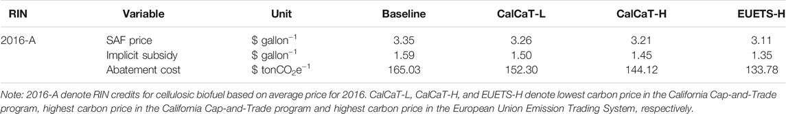
TABLE 7. GHG emission abatement costs with conversion yield of 29.40 gallons ton−1.
At a 29.40 gallons ton−1 conversion rate, the aggregate net farm income decreases given less feedstock demand compared to the Baseline conversion rate, resulting in an economic loss of nearly $17 million to the feedstock producers. Without carbon credits, social cost of aviation GHG emissions is around $26.0 million, resulting in a net supply-chain welfare of about -$211.3 million and $45.7 million with 2016-A and 2017-A RIN credits, respectively. The net supply-chain welfare under the three carbon credit scenarios increases from $3.2 million to $33.4 million compared to the Baseline. Displacing CJF with the ATJ-pathway SAF from switchgrass with a conversion yield of 29.40 gallons ton−1 reduces the total LCA-based GHG emissions by 63% under the Baseline. With carbon credits, the total GHG emission reductions from using SAF and its co-products reach to 64.5–66% for the three carbon credits scenarios compared to the CJF usage in the aviation sector.
Conclusion
Given the rising interest in reducing GHG emissions from the aviation sector, the implications of costs, GHG emissions, and welfare associated with commercial-scale switchgrass-based SAF under the ATJ-pathway are analyzed. Impacts of SAF production from switchgrass on farmland allocation, processing facility configuration, and GHG emissions are estimated assuming a bi-level Stackelberg model to incorporate possible interaction amongst the participants. Using an ex-ante analysis for a case study that targets the MEM, the differences in the optimal decisions of a SAF processor and its contracted feedstock producers are evaluated under a with- and without-hypothetical carbon credit scenarios. The potential impacts of several carbon credit scenarios on the optimal decisions of the feedstock producers and the processor are evaluated in terms of changes in the LCA-based GHG emissions and net supply-chain welfares.
The feedstock producers’ annual economic surplus is about $16.9 million for the no carbon credit case (i.e., Baseline) with the majority of the feedstock producers receiving a margin ranging from 10 to 47% over their opportunity costs of land conversion. Under the case of available carbon credits, the processor’s cost decreases by $17.7 to $59.5 million annually from the Baseline. Since the SAF processor’s optimal decisions includes feedstock producers converting higher opportunity cost crop lands to switchgrass production, a decline of $5.9 to $10.5 million annually in the aggregate feedstock producer surplus incures when compared to the Baseline. On the other hand, airlines reduces negative economic surplus because of lower SAF price given carbon and RIN credits. The net supply-chain welfare increases by $12.7 to $50.6 million annually under the carbon credit scenarios irrespective of the level of RIN credits.
Replacing the CJF and other fossil fuels with SAF and its co-products from the ATJ-pathway could lead to 62.5–65.0% LCA-based GHG emission reductions. We obtain a range of 31.37–33.37 gCO2e MJ−1 by replacing the CJF and other fossil fuels with SAF and its co-products from the switchgrass-based ATJ-pathway. The west Tennessee estimates is slightly higher than the values of the International Civil Aviation Organization Carbon Offsetting and Reduction Scheme for International Aviation (2021), which is 28.90 gCO2e MJ−1 for LCA-based GHG emission associated with the U.S. switchgrass-based ATJ-pathway.
Utilizing SAF and its co-products is important to achieving IATA’s goal of lowering 50% GHG emissions by 2050 relative to the 2005 level. However, the potential environmental benefits would not be achieved without cost. Estimated GHG emission abatement costs, ranging from $151 to 198 tonCO2e−1, imply that the stakeholders of the aviation sector, including policy makers, feedstock and SAF producers, and the airlines, must come together and share the responsibility to help the decarbonization from the sector. In addition, the sensitivity analysis suggests increasing SAF conversion rate from biomass could largely lower the SAF break-even and enhance the competitiveness of SAF over CJF.
Data Availability Statement
The original contributions presented in the study are included in the article/Supplementary Material, further inquiries can be directed to the corresponding author.
Author Contributions
BS is responsible for the analysis and interpretation of data for the work, and drafting the work; TY initiates the conception of the work and revises the manuscript critically; BE and CB provide approval for publication of the content; all authors agree to be accountable for all aspects of the work.
Funding
This work is partially funded by the US Federal Aviation Administration (FAA) Office of Environment and Energy as a part of ASCENT Project 1 under FAA Award Number: 13-C-AJFEUTENN-Amd 5. Any opinions, findings, and conclusions or recommendations expressed in this material are those of the authors and do not necessarily reflect the views of the FAA or other ASCENT sponsor organizations.
Conflict of Interest
The authors declare that the research was conducted in the absence of any commercial or financial relationships that could be construed as a potential conflict of interest.
Publisher’s Note
All claims expressed in this article are solely those of the authors and do not necessarily represent those of their affiliated organizations, or those of the publisher, the editors and the reviewers. Any product that may be evaluated in this article, or claim that may be made by its manufacturer, is not guaranteed or endorsed by the publisher.
Supplementary Material
The Supplementary Material for this article can be found online at: https://www.frontiersin.org/articles/10.3389/fenrg.2021.775389/full#supplementary-material
Footnotes
1Offtake agreements are contracts between fuel consumers and producers specifying the procurement of specified fuel volumes for a period and have recently been agreed upon with several airlines [Commercial Aviation Alternative Fuels Initiative (CAAFI), 2016].
2The GHG emissions from feedstock production through SAF delivery to the airport is considered as the LCA-based emission because GHG emissions from burning biomass-based renewable fuel nearly equal the amount of CO2 sequestered by the biomass during its growth, i.e. biogenic carbon (Elgowainy et al., 2012; Wang et al., 2012).
3The profit margin is approximated based on the percentage of refining costs and profits of average retail price paid for gasoline in the U.S for 2008–2017 (U.S. Energy Information Administration (EIA), 2017), and the average retail price for CJF in the year 2017 [Bureau of Transportation Statistics (BTS), 2016a].
4Total fuel consumption at the Memphis airport (MEM) was estimated around 410 million gallons in 2016 (Pearlson, 2020). The assumed SAF demand is close to 33% of the total jet fuel consumption, which is under the current statutory blending limit (50%) for the ATJ pathway
5Advanced biofuels such as biomass-based biodiesel (BBD) counts as 1.5 or 1.7 RINS (depending on fuel type) to reflect its higher energy content compared to ethanol (Congressional Research Service, 2013). The available RIN prices on cellulosic ethanol are multiplied by a factor of 1.7 for generating cellulosic SAF-based RIN credits
6The SAF break-even price level without the RIN credits remains above $7.5/gallon which is generally higher compared to the ones estimated in the recent SAF studies (e.g., Tao et al., 2017; Yao et al., 2017) as the minimal profitability expectation of the individual feedstock producers are satisfied given the game-theoretic interaction between the feedstock producers and the processor
References
Agusdinata, D. B., Zhao, F., Ileleji, K., and DeLaurentis, D. (2011). Life Cycle Assessment of Potential Biojet Fuel Production in the United States. Environ. Sci. Technol. 45 (21), 9133–9143. doi:10.1021/es202148g
Alternative Fuels Data Center (AFDC) (2017). Alternative Fuel Price Report. Washington, DC: U.S. Department of Energy. Retrieved from https://www.afdc.energy.gov/uploads/publication/alternative_fuel_price_report_oct_2017.pdf.
Argone National Laboratory (2017). The Greenhouse Gases, Regulated Emissions, and Energy Use in Transportation Model (GREET). Retrieved from http://www.transportation.anl.gov/publications/index.html.
Bai, Y., Ouyang, Y., and Pang, J.-S. (2012). Biofuel Supply Chain Design under Competitive Agricultural Land Use and Feedstock Market Equilibrium. Energ. Econ. 34 (5), 1623–1633. doi:10.1016/j.eneco.2012.01.003
Bann, S. J., Malina, R., Staples, M. D., Suresh, P., Pearlson, M., Tyner, W. E., et al. (2017). The Costs of Production of Alternative Jet Fuel: A Harmonized Stochastic Assessment. Bioresour. Techn. 227, 179–187. doi:10.1016/j.biortech.2016.12.032
Boyer, C. N., Roberts, R. K., English, B. C., Tyler, D. D., Larson, J. A., and Mooney, D. F. (2013). Effects of Soil Type and Landscape on Yield and Profit Maximizing Nitrogen Rates for Switchgrass Production. Biomass and Bioenergy 48, 33–42. doi:10.1016/j.biombioe.2012.11.004
Boyer, C. N., Tyler, D. D., Roberts, R. K., English, B. C., and Larson, J. A. (2012). Switchgrass Yield Response Functions and Profit‐Maximizing Nitrogen Rates on Four Landscapes in Tennessee. Agron.j. 104 (6), 1579–1588. doi:10.2134/agronj2012.0179
Bureau of Transportation Statistics (BTS) (2016a). Airlines and Airports. Washington, DC: U.S. Department of Transportation. Retrieved from https://www.transtats.bts.gov/NewAirportList.asp?xpage=airports.asp&flag=FACTS.
California Carbon Dashboard (2018). Carbon Price. Retrieved from http://calcarbondash.org/csv/output.csv.
Chen, X., Huang, H., Khanna, M., and Önal, H. (2011). The Intended and Unintended Effects of US Agricultural and Biotechnology Policies. University of Chicago Press, 223–267. doi:10.3386/w16697Meeting the Mandate for Biofuels: Implications for Land Use, Food, and Fuel Prices
Commercial Aviation Alternative Fuels Initiative (CAAFI) (2016). 2016 Biennial General Meeting. Retrieved from http://caafi.org/information/pdf/Biennial_Meeting_Oct252016_Opening_Remarks.pdf.
Congressional Research Service (2013). Renewable Fuel Standard: Overview and Issues. Retrieved from https://www.ifdaonline.org/IFDA/media/IFDA/GR/CRS-RFS-Overview-Issues.pdf.
Elgowainy, A., Han, J., Wang, M., Carter, N., Stratton, R., Hileman, J., et al. (2012). Life-cycle Analysis of Alternative Aviation Fuels in GREET. Argonne, IL: Argonne National Laboratory (ANL.
Grote, M., Williams, I., and Preston, J. (2014). Direct Carbon Dioxide Emissions from Civil Aircraft. Atmos. Environ. 95, 214–224. doi:10.1016/j.atmosenv.2014.06.042
Gümüş, Z. H., and Floudas, C. A. (2005). Global Optimization of Mixed-Integer Bilevel Programming Problems. Comput. Manage. Sci. 2 (3), 181–212.
Han, J., Tao, L., and Wang, M. (2017). Well-to-wake Analysis of Ethanol-To-Jet and Sugar-To-Jet Pathways. Biotechnol. Biofuels 10 (1), 21. doi:10.1186/s13068-017-0698-z
Intergovernmental Panel on Climate Change. (IPCC) (2014). synthesis report, contribution of working groups I, II and III to the Fifth assessment report of the intergovernmental panel on climate change. Editors R. K. Pachauri, and L. A. Meyer. Geneva, Switzerland: IPCC. Retrieved from https://www.ipcc.ch/site/assets/uploads/2018/02/AR5_SYR_FINAL_SPM.pdf.
Intergovernmental Panel on Climate Change. (IPCC) (2018). Summary for Policymakers of IPCC Special Report on Global Warming of 1.5°C. Retrieved from https://www.ipcc.ch/2018/10/08/summary-for-policymakers-of-ipcc-special-report-on-global-warming-of-1-5c-approved-by-governments/.
International Air Transport Association (IATA) (2017). Fact Sheet: Alternative Fuels. Retrieved from https://www.iata.org/pressroom/facts_figures/fact_sheets/Documents/fact-sheet-alternative-fuels.pdf.
International Air Transport Association (IATA) (2015). IATA Sustainable Aviation Fuel Roadmap. Retrieved from https://www.iata.org/whatwedo/environment/Documents/safr-1-2015.pdf.
International Civil Aviation Organization (ICAO) (2021). Carbon Offsetting and Reduction Scheme for International Aviation (CORSIA). Retrieved from https://www.icao.int/environmental-protection/CORSIA/Documents/ICAO%20document%2006%20-%20Default%20Life%20Cycle%20Emissions%20-%20March%202021.pdf.
Jager, H. I., Baskaran, L. M., Brandt, C. C., Davis, E. B., Gunderson, C. A., and Wullschleger, S. D. (2010). Empirical Geographic Modeling of Switchgrass Yields in the United States. GCB Bioenergy 2 (5), 248–257. doi:10.1111/j.1757-1707.2010.01059.x
Lim, M. K., and Ouyang, Y. (2016). “Biofuel Supply Chain Network Design and Operations,” in Environmentally Responsible Supply Chains. Springer Series in Supply Chain Management. Editor A. Atasu (Cham: Springer), Vol. 3, 143–162. doi:10.1007/978-3-319-30094-8_9
Luo, Y., and Miller, S. (20132013). A Game Theory Analysis of Market Incentives for US Switchgrass Ethanol. Ecol. Econ. 93, 42–56. doi:10.1016/j.ecolecon.2013.04.015
Melissae Fellet, M. (2016). Aviation Industry Hopes to Cut Emissions with Jet Biofuel. C&EN Glob. Enterp 94 (37), 16–18. doi:10.1021/cen-09437-scitech1
Nordhaus, W. D. (2017). Revisiting the Social Cost of Carbon. Proc. Natl. Acad. Sci. USA 114 (7), 1518–1523. doi:10.1073/pnas.1609244114
O'Connell, A., Kousoulidou, M., Lonza, L., and Weindorf, W. (2019). Considerations on GHG Emissions and Energy Balances of Promising Aviation Biofuel Pathway. Renew. Sust. Energ. Rev 101, 504–515.
Perlack, R. D., Eaton, L. M., Turhollow, A. F., Langholtz, M. H., Brandt, C. C., Downing, M. E., et al. (2011). US Billion-Ton Update: Biomass Supply for a Bioenergy and Bioproducts Industry.
Reimer, J. J., and Zheng, X. (2017). Economic Analysis of an Aviation Bioenergy Supply Chain. Renew. Sust. Energ. Rev. 77, 945–954. doi:10.1016/j.rser.2016.12.036
Renewable Fuels Association (RFA) (2017). Renewable Fuel Standard Program: Standards for 2018 and Biomass-Based Diesel Volume for 2019. Retrieved from http://www.ethanolrfa.org/wp-content/uploads/2017/08/RFA-Comments_2018-RVO-Proposed-Rule_Final.pdf.
Intergovernmental Panel on Climate Change. (IPCC) (2014). in Climate Change 2014: Synthesis Report, Contribution of Working Groups I, II and III to the Fifth Assessment Report of the Intergovernmental Panel on Climate Change [Core Writing Team. Editors R. K. Pachauri, and L. A. Meyer (Geneva, Switzerland: IPCC). Retrieved from https://www.ipcc.ch/site/assets/uploads/2018/02/AR5_SYR_FINAL_SPM.pdf.
Sinha, A., Malo, P., and Deb, K. (2018). A Review on Bilevel Optimization: from Classical to Evolutionary Approaches and Applications. IEEE Trans. Evol. Computat. 22, 276–295. doi:10.1109/tevc.2017.2712906
Staples, M. D., Malina, R., Olcay, H., Pearlson, M. N., Hileman, J. I., Boies, A., et al. (2014). Lifecycle Greenhouse Gas Footprint and Minimum Selling price of Renewable Diesel and Jet Fuel from Fermentation and Advanced Fermentation Production Technologies. Energy Environ. Sci. 7 (5), 1545–1554. doi:10.1039/c3ee43655a
Staples, M. D., Malina, R., Suresh, P., Hileman, J. I., and Barrett, S. R. H. (2018). Aviation CO2 Emissions Reductions from the Use of Alternative Jet Fuels. Energy Policy 114, 342–354. doi:10.1016/j.enpol.2017.12.007
Tao, L., Markham, J. N., Haq, Z., and Biddy, M. J. (2017). Techno-economic Analysis for Upgrading the Biomass-Derived Ethanol-To-Jet Blendstocks. Green. Chem. 19 (4), 1082–1101. doi:10.1039/c6gc02800d
U.S. Energy Administration System (EIA) (2017). Gasoline and Disesl Fuel Update. https://www.eia.gov/energyexplained/index.php?page=gasoline_factors_affecting_prices.
U.S. Environmental Protection Agency. (EPA) (2017). Climate Change: Basic Information. https://19january2017snapshot.epa.gov/climatechange/climate-change-basic-information_.html.
U.S. Federal Aviation Administration (FAA) (2017). History of Alternative Jet Fuel Use. https://www.faa.gov/nextgen/where_we_are_now/nextgen_update/images/pp_ee_sb1_body1.png.
Wang, M., Han, J., Dunn, J. B., Cai, H., and Elgowainy, A. (2012). Well-to-wheels Energy Use and Greenhouse Gas Emissions of Ethanol from Corn, Sugarcane and Cellulosic Biomass for US Use. Environ. Res. Lett. 7 (4), 045905. doi:10.1088/1748-9326/7/4/045905
Wang, M., Huo, H., and Arora, S. (2011). Methods of Dealing with Co-products of Biofuels in Life-Cycle Analysis and Consequent Results within the U.S. Context. Energy Policy 39 (10), 5726–5736. doi:10.1016/j.enpol.2010.03.052
Winchester, N., Malina, R., Staples, M. D., and Barrett, S. R. H. (2015). The Impact of Advanced Biofuels on Aviation Emissions and Operations in the U.S. Energ. Econ. 49, 482–491. doi:10.1016/j.eneco.2015.03.024
Winchester, N., McConnachie, D., Wollersheim, C., and Waitz, I. A. (2013). Economic and Emissions Impacts of Renewable Fuel Goals for Aviation in the US. Transportation Res. A: Pol. Pract. 58, 116–128. doi:10.1016/j.tra.2013.10.001
Wright, L., and Turhollow, A. (2010). Switchgrass Selection as a "model" Bioenergy Crop: A History of the Process. Biomass and Bioenergy 34, 851–868. doi:10.1016/j.biombioe.2010.01.030
Yao, G., Staples, M. D., Malina, R., and Tyner, W. E. (2017). Stochastic Techno-Economic Analysis of Alcohol-To-Jet Fuel Production. Biotechnol. Biofuels 10 (1), 18. doi:10.1186/s13068-017-0702-7
Yao, H., Mai, T., Wang, J., Ji, Z., Jiang, C., and Qian, Y. (2019). Resource Trading in Blockchain-Based Industrial Internet of Things. IEEE Trans. Ind. Inf. 15 (6), 3602–3609. doi:10.1109/tii.2019.2902563
Yu, T. E., English, B. C., He, L., Larson, J. A., Calcagno, J., Fu, J. S., et al. (2016). Analyzing Economic and Environmental Performance of Switchgrass Biofuel Supply Chains. Bioenerg. Res. 9 (2), 566–577. doi:10.1007/s12155-015-9699-6
Keywords: sustainable aviation fuel (SAF), stackelberg model, carbon credit, land use, land cover change, GHG emissions
Citation: Sharma BP, Yu TE, English BC and Boyer CN (2021) Economic Analysis of Developing a Sustainable Aviation Fuel Supply Chain Incorporating With Carbon Credits: A Case Study of the Memphis International Airport. Front. Energy Res. 9:775389. doi: 10.3389/fenrg.2021.775389
Received: 13 September 2021; Accepted: 08 November 2021;
Published: 09 December 2021.
Edited by:
Kristin C. Lewis, Volpe National Transportation Systems Center, United StatesReviewed by:
Bheru Lal Salvi, Maharana Pratap University of Agriculture and Technology, IndiaDenny K. S. NG, Heriot-Watt University Malaysia, Malaysia
Copyright © 2021 Sharma, Yu, English and Boyer. This is an open-access article distributed under the terms of the Creative Commons Attribution License (CC BY). The use, distribution or reproduction in other forums is permitted, provided the original author(s) and the copyright owner(s) are credited and that the original publication in this journal is cited, in accordance with accepted academic practice. No use, distribution or reproduction is permitted which does not comply with these terms.
*Correspondence: T. Edward Yu, dHl1MUB1dGsuZWR1