A Hybrid Model for Power Consumption Forecasting Using VMD-Based the Long Short-Term Memory Neural Network

Energy consumption prediction is a popular research field in computational intelligence. However, it is difficult for general machine learning models to handle complex time series data such as building energy consumption data, and the results are often unsatisfactory. To address this difficulty, a hybrid prediction model based on modal decomposition was proposed in this paper. For data preprocessing, the variational mode decomposition (VMD) technique was used to used to decompose the original sequence into more robust subsequences. In the feature selection, the maximum relevance minimum redundancy (mRMR) algorithm was chosen to analyse the correlation between each component and the individual features while eliminating the redundancy between individual features. In the forecasting module, the long short-term memory (LSTM) neural network model was used to predict power consumption. In order to verify the performance of the proposed model, three categories of contrast methods were applied: 1) Comparing the hybrid model to a single predictive model, 2) Comparing the hybrid model with the backpropagation neural network (BPNN) to the hybrid model with the LSTM and 3) Comparing the hybrid model using mRMR and the hybrid model using mutual information maximization (MIM). The experimental results on the measured data of an office building in Qingdao show that the proposed hybrid model can improve the prediction accuracy and has better robustness compared to VMD-MIM-LSTM. In the three control groups mentioned above, the R² value of the hybrid model improved by 10, 3 and 3%, respectively, the values of the mean absolute error (MAE) decreased by 48.9, 41.4 and 35.6%, respectively, and the root mean square error (RMSE) decreased by 54.7, 35.5 and 34.1%, respectively.

1 Introduction

Energy is critical in modern society, and energy consumption is a major issue that has long plagued humanity. Increasing demand for energy is gradually drawing attention to energy conservation issues around the world. Among energy sources, building electricity consumption accounts for a large proportion of total social energy consumption. From a global perspective, building energy consumption accounts for about 40% of the global energy consumption, and this proportion is likely to increase in the future.

Scientists have explored various methods for predicting building electricity consumption, aiming to achieve intelligent energy management and energy-saving building reconstruction based on predicted energy consumption. However, building electricity forecasting continues to be a challenging effort due to the variety of factors that affect energy consumption, such as building structure, equipment, weather conditions, and energy-use behaviours of the building occupants.

Building electricity consumption predictions can be divided into three methods according to the type of data input and processing method used: White-box physics-based models, grey-box reduced-order models and black-box data-driven models.

White-box physics-based models rely on thermodynamic rules for detailed energy modelling and analysis. The construction of the physical model requires a large number of physical parameters related to the building and a detailed setting of the system operation. Its accuracy depends on the input parameters and the selected simulation software. Zhu et al. (Zhu et al., 2012; Said, 2016) compared the Dest, Energy Plus and DOE-2 simulation software calculation methods, and their research results showed that the difference of load between the simulation results of Dest and Energy Plus was less than 10%. However, some detailed architectural data may not be readily available to researchers, resulting in an inability to provide accurate inputs and thus leading to poor predictive performance.

Grey-box modelling approaches offer a combination of physical and data-driven prediction models, leveraging the advantages and minimizing the disadvantages of both approaches. In grey-box models, some internal parameters and equations are physically interpretable (Eom et al., 2012; Amasyali and El-Gohary, 2018). Grey-box models may also show better performance compared to black-box and white-box models. For example, Dong et al. (Dong et al., 2016) developed a hybrid model which coupled a data-driven model and a thermal network model for predicting the total energy consumption of residential areas and compared its prediction performance to artificial neural networks (ANN), support vector machines (SVM) and least square support vector machine (LSSVM)-based models.

Unlike physical models, black-box data-driven models do not require detailed building data, but rather they learn from the available historical data to make predictions. Common machine learning algorithms include SVM and ANN. These algorithms have a wide range of applications in the field of energy consumption prediction. Currently, about 47% of studies use ANN to predict energy consumption (Liu et al., 2019). For example, Mansoor et al. (Muhammad et al., 2020) compared two different neural network models, feed-forward neural networks (FFNN) and echo state networks (ESN) for electrical load forecasting in real commercial buildings; their results indicated that the ESN model generally performed slightly better than the FFNN model Katarina. Liu et al. (Liu et al., 2020) proposed a hybrid forecasting model that combined the Jaya algorithm and SVM. In this model, the representative features of the input data were selected and the hyper-parameters of SVM were optimized by using the Jaya optimization algorithm to efficiently improve the forecasting accuracy of wind speed. Mendonça et al. (de Paiva et al., 2020) investigated the application of machine learning models for solar radiation intensity prediction. They evaluated multigene genetic programming (MGGP) and the multilayer perceptron (MLP) ANN. The results showed that MGGP produced better results in the case of a single prediction, while ANN presented more accurate results for ensemble forecasting. Anderso et al. (Marcello Anderson et al., 2017) applied portfolio theory to solar and wind energy forecasting to improve resource forecasting for specific solar and wind energy conditions in the Brazilian region. Their study showed that the optimal combination of 30% solar and 70% wind resources generated the smallest calculated standard deviation.

However, the original time series were often unstable due to the disturbance of uncertainty. For this type of data, a single model did not produce excellent results (He et al., 2018). To improve the prediction accuracy, the segregation of these series with different frequencies from the energy data was considered as a possible solution.

Empirical mode decomposition (EMD) was proposed by Dr Norden E. Huang in 1998 (Huang Norden et al., 1998) as a method for processing nonstationary signals; it is an adaptive time-frequency localization analysis method, the number of decomposed IMFs depends on the data itself. Liu et al. (Liu et al., 2012) proposed a standard hybridization of EMD with the backpropagation neural network (BPNN) method. In this study, all intrinsic mode functions (IMFs) and the residue were forecasted with BPNN models. Similarly, Guo et al. (Guo et al., 2011) proposed a modified EMD–FFNN model in the form of an EMD-based FFNN ensemble learning paradigm. This study showed that the first IMF containing high-frequency components was mostly unsymmetrical and disordered, which led to the generation of large forecasting disturbances. The simplest combinations of hybrid EMD–SVM models are presented in the literature (Lin and Peng, 2011; Zhang et al., 2015). These models decomposed wind data into a series of components (IMFs) using EMD, and then different models were built with various kernel functions and parameters for each component using the SVM model.

However, the IMF components obtained by EMD often exhibit mode mixing, resulting in inaccurate IMF components. To solve this problem, many scholars have proposed improved algorithms. Wu and Huang (Wu and Huang, 2009) suggested the ensemble empirical mode decomposition (EEMD) method. Numerous articles in distinct research areas have claimed the superior performance of the EEMD method over hybrid EMD models. The hybrid EEMD–SVM model has been used in the literature and has achieved better prediction accuracy than other models (Hu et al., 2013; Wu et al., 2018). In one work (Wu et al., 2018), wind speed data was decomposed into seven IMF components with EEMD and then the IMFs were predicted using the appropriate SVM models. Elsewhere, a similar approach was used in which the first IMF (IMF1) was removed from the prediction analysis and all remaining IMFs were forecasted with SVM models (Hu et al., 2013). Yu et al. (Wu et al., 2018) proposed a novel model based on EEMD and LSTM for crude oil price forecasting. In this study, a method to select the same number of proper inputs in various decomposition scenarios was developed. To extract features from the selected components more adequately, LSTM was introduced as a forecasting method to predict price movement directly. Dragomiretskiy and Zosso (Dragomiretskiy and Zosso, 2014) introduced the variational mode decomposition (VMD) method in 2014. The VMD algorithm is more robust in that it inherits the advantages of the EMD algorithm while solving the mode mixing problem of the EMD algorithm. In recent years, the VMD algorithm has been successfully applied in many fields, such as fault diagnosis research (Zhang et al., 2017) and forecast research (Liu et al., 2018; Niu et al., 2020). The studies of He (He et al., 2019) and Li (Li et al., 2018) have shown that the combination model based on “decomposition-prediction” can achieve high prediction accuracy in heating and cooling seasons. He et al. developed a VMD-LSTM forecasting model for electricity load forecasting in Hubei province. They divided the 1-year data into four parts, corresponding to four seasons. The results show that the proposed forecasting model has high forecasting accuracy on all four data sets. The lowest prediction accuracy is found in summer, attributed to the higher fluctuation and uncertainty of load in summer.

Studies using signal decomposition methods have some shortcomings. Firstly, some literature uses different prediction methods for different IMF frequencies while ignoring the feature selection variability of IMFs. Secondly, it is difficult to provide a reasonable explanation for the physical meaning of each component using signal decomposition methods. To address these inadequacies, a hybrid system was developed that comprises three modules to predict the electricity load of public buildings in Qingdao. Compared with existing studies on short-term load forecasting, the main contributions of this paper are as follows:

1) A novel deep learning-based method for predicting building electricity consumption is proposed. The idea of ‘‘decomposition–reconstruction–integration” results in a feasible and efficient method to model and forecast nonlinear, non-stationary, complex time series.

2) Due to the volatility and uncertainty of the load data, VMD is used to decompose the raw load into more stable series. Most of the literature does not detail the determination of the number of VMD components (Sun et al., 2019b). In this paper, the mean value of the instantaneous frequency of each component is used to determine the number of K.

3) Most of the literature does not provide a reasonable interpretation of the components decomposed by the modal decomposition algorithm. In this paper, the highly volatile load is decomposed into several subsequences by VMD. The redundancy between features is removed by the mRMR algorithm so that each subsequence has a suitable feature. With the features selected by mRMR, this paper attempts to analyse the physical meaning of each subsequence.

This study is organized as follows. Section 2 outlines the principles of the methods related to the proposed hybrid system. In addition, a case study is presented in Section 3. Finally, the study’s conclusions and avenues for future work are presented in Section 4. Note that the data decomposition and feature selection were performed on a laptop with an Intel(R) i5-7400 CPU with MATLAB 2020a installed, and the deep learning model was performed on a laptop with an Intel(R) i5-7400 CPU with Python 3.8 installed.

2 Methodology

The main contents of this section introduce the algorithm used in this paper: Variational mode decomposition (VMD), Max-Relevance and Min-Redundancy (mRMR) and Long Short-Term Memory Neural Network (LSTM). The flow chart of the hybrid model is shown in Figure 1.

FIGURE 1

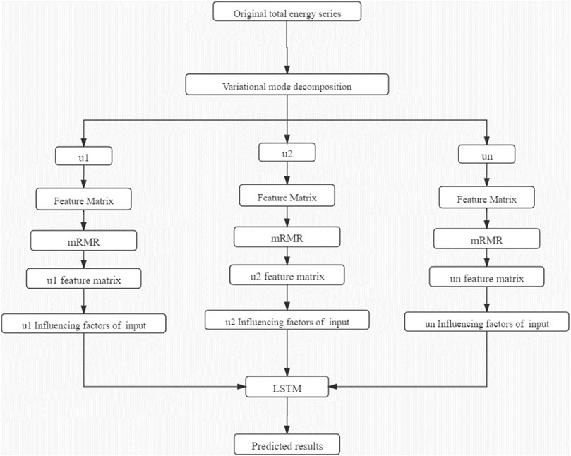
FIGURE 1. Hybrid model flow chart.

2.1 Principle of Variational Mode Decomposition

2.1.1 VMD Principle

In order to solve the modal mixing problem existing in EMD, Dragomiretskiy et al. (Dragomiretskiy and Zosso, 2014) proposed the VMD algorithm, which is essentially a set of adaptive Wiener filter sets. The decomposition number K of VMD is determined artificially. Theoretically, if the value of K is more reasonable, it can effectively suppress the modal mixing phenomenon. the main process of VMD is divided into five steps:

1) Suppose $u_k$ is the Kth order mode of the original signal $f$ and $\delta \left(t\right)$ is a Dirac distribution. The analytic signal of the mode $u_k$ is calculated by Hilbert transform, then its unilateral frequency spectrum can be expressed as:

$\left(\delta \left(t\right)+\frac{j}{\pi t}\right)\text{*}{u}_k\left(t\right)(1)$

2) Adding a pre-estimated center frequency to the resolved signal of the mode, the frequency of the mode can be modulated to the corresponding baseband:

$\left[\left(\delta \left(t\right)+\frac{j}{\pi t}\right)\text{*}{u}_k\left(t\right)\right]e^{-j{w}_{k}t}(2)$

3) Calculating the bandwidth of each modal signal, the constrained optimization problem is expressed as:

$\underset{\left\{u_k\right\},\left\{w_k\right\},}{\text{min}}\left\{{\displaystyle \sum _{k=1}^k\Vert {\sigma }_t}\left[\left(\delta \left(t\right)+\frac{j}{\pi t}\right)\text{*}{u}_k\left(t\right)\right]e^{-j{w}_{k}t}{\Vert }_2^2\right\}(3)$

where the constraint of Eq. 3 is: ${\displaystyle \sum _{k=1}^k{u}_k}\left(t\right)=f\left(t\right)$.

4) The Lagrangian function $\lambda \left(t\right)$ and quadratic penalty factor $\alpha$ are introduced to solve the optimal solution of the constrained problem and transform the constrained optimization problem into an unconstrained optimization problem.

$L\left[\left\{u_k\right\},\left\{w_k\right\},\lambda \right]=\alpha {\displaystyle \sum _{k=1}^k\Vert {\sigma }_t}\left[\left(\delta \left(t\right)+\frac{j}{\pi t}\right)\text{*}{u}_k\left(t\right)\right]e^{-j{w}_{k}t}{\Vert }_2^2+\Vert f\left(t\right)-{\displaystyle \sum _{k=1}^k{u}_k}\left(t\right){\Vert }_2^2+\langle \lambda \left(t\right),f\left(t\right)-{\displaystyle \sum _{k=1}^k{u}_k}\left(t\right)\rangle (4)$

5) Use the multiplicative operator alternating direction method to update $u_k^{n+1}$, $w_k^{n+1}$, ${\lambda }^{n+1}$ alternately in both directions until the following iteration conditions are satisfied:

${\displaystyle \sum _k\Vert {\stackrel{\wedge }{u}}_k^{n+1}-{\stackrel{\wedge }{u}}_k^n{\Vert }_2^2/\Vert {\stackrel{\wedge }{u}}_k^n{\Vert }_2^2}<\epsilon (5)$

Where $\epsilon >0$, $u_k^{n+1}$, $w_k^{n+1}$, ${\lambda }^{n+1}$ are denoted as:

${\widehat{u}}_k^{n+1}\left(w\right)=\frac{\widehat{f}\left(\omega \right)-{\displaystyle {\sum }_{i<k}{\widehat{u}}_k^{n+1}}\left(\omega \right)-{\displaystyle {\sum }_{i>k}{\widehat{u}}_k^n\left(\omega \right)}+\frac{{\widehat{\lambda }}^n\left(w\right)}{2}}{1+2\alpha {\left(\omega -{\omega }_k^n\right)}^2}(6)$

${\omega }_k^{n+1}=\frac{{{\displaystyle \int }}_0^{\infty }\omega {\left|{\widehat{u}}_k^{n+1}\left(w\right)\right|}^{2}d\omega }{{{\displaystyle \int }}_0^{\infty }{\left|{\widehat{u}}_k^{n+1}\left(w\right)\right|}^{2}d\omega }(7)$

${\widehat{\lambda }}^{n+1}\left(\omega \right)={\widehat{\lambda }}^n\left(\omega \right)+\tau \left(\widehat{f}\left(w\right)-{\widehat{u}}_k^{n+1}\left(\omega \right)\right)(8)$

where $\tau$ is the updated noise parameter.

2.1.2 VMD parameter determination

1) Modal Number

The number of modalities K should be determined before the VMD is used to decompose. Too large or too small a value of K will affect the accuracy of the model. In this paper, the mean value of instantaneous frequency of each component is used to determine the number of K. When the value of k is too large, and the high-frequency component will be broken. It means that the instantaneous frequency at the break of the high-frequency component is 0. As a result, the high-frequency component breaks lead to a decrease in the average instantaneous frequency. Figure 2 shows the mean values of instantaneous frequencies for the nine cases of VMD components. It can be seen from the figure that the number of VMD components increases to a certain number, and the curve has an obvious bending phenomenon. To sum up, the value of K is chosen as 4.

2) Penalty Factor

FIGURE 2

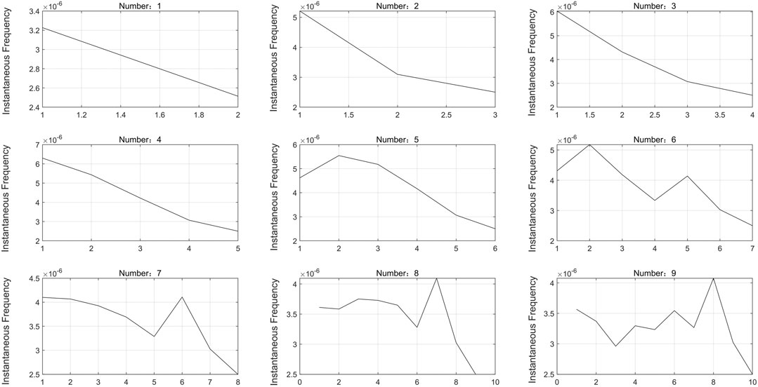
FIGURE 2. Average instantaneous frequency when K from 1 to 9

The penalty factor changes the constrained variational problem into a non-constrained variational problem. According to Ref. (Wu, 2016), when the value of the penalty factor is set to 2000 has strong adaptability and can ensure a certain convergence speed.

2.2 Principle of Max-Relevance and Min-Redundancy

Peng et al.(Peng et al., 2005) proposed a feature selection method based on Mutual Information, which uses Mutual Information to measure the dependency between two variables while taking into account the redundancy between features.

2.2.1 Max-Relevance

The maximum correlation criterion solution can be expressed as the average of the mutual information between the feature $x_i$ and the target variable $y$:

$\text{max}D\left(J,y\right)=\frac{1}{\left|J\right|}{\displaystyle \sum }_{x_i\in J}I\left(x_i,y\right)(9)$

where $x_i$ is the characteristic; $y$ represents the target variable; $J$ is the set containing the $x_i$; $I\left(x_i,y\right)$ represents the mutual information between the feature $x_i$ and the target variable $y$. The expression is as follows:

$I\left(x_i,y\right)={\displaystyle \int {\displaystyle \int p\left(x_i,y\right)}}\text{log}\frac{p\left(x_i,y\right)}{p\left(x_i\right)p\left(y\right)}d{x}_{i}dy(10)$

where $p\left(x_i\right),p\left(y\right)$ are the edge probability density functions of $x_i$ and $y$, respectively $,p\left(x_i,y\right)$ is the joint probability density function of of $x_i$ and $y$.

2.2.2 Minimum Redundancy

The overlapping information between any two feature variables is called redundancy information. The features selected according to Eq. 9 only consider the degree of correlation and do not consider the existence of redundancy between features. The input of redundant features increases the number of input features, and decreases the accuracy of the prediction model. The Minimum Redundancy expression is as follows:

$\min R\left(J\right)=\frac{1}{{\left|J\right|}^2}{\displaystyle \sum _{x_i\in J,x_j\in J}I\left(x_i,x_j\right)}(11)$

mRMR can be expressed by Eqs 9, 11 as:

$\max \psi \left(D,R\right),\psi =D-R.(12)$

2.3 Prediction Model

The prediction part uses Long Short-Term Memory Neural Network (LSTM) model, which was proposed by Hochreiter and Schmidhuber (Hochreiter and Schmidhuber, 1997) to learn long-term dependence information. It can handle more complex problems, and has more mature applications in the field of load prediction (Sun et al., 2019a). Long short-term memory neural network is a special form of the recurrent neural network. LSTM is composed of cells with the same structure (Figure 3). In this model, the data of the next moment is predicted each time by the previous data and historical data, which is processed by the cells. Each cell has three input parameters: Historically stored information $C_{t-1}$, historical data $X_t$ and $h_{t-1}$, which represent the prediction results of the last cell and input parameter to the cell. Each cell contains four parts, including the forgotten gate, the input gate, the update gate and the output gate.

FIGURE 3

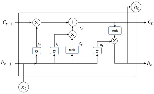
FIGURE 3. LSTM structure.

The data $h_{t-1}$ that processed by the previous cell, and the input data of the current time $X_t$ are linked by a matrix and obtain $X_t^{\text{'}}$,

${X^{\text{'}}}_t=\left[h_{t-1},X_t\right](13)$

In the forgotten gate, LSTM can decide what information to discard from the cell. After the sigmoid function processing, $X_t^{\text{'}}$ can get $f_{t1}$. LSTM can remember large amounts of historical data by $f_{t1}$ filtered data.

$f_{t1}=\sigma \left(W_f\cdot X^{\text{'}}+b_f\right)(14)$

In the input gate, LSTM acquires the new data, After the sigmoid function processing, $X_t^{\text{'}}$ can get $i_t$. The $i_t$ decides the useful data in $X_t^{\text{'}}$. Moreover, $X_t^{\text{'}}$ is processed by the tanh function to calculate $C_t^{\text{'}}$,

$i_t=\sigma \left(W_i\cdot X^{\text{'}}+b_t\right)(15)$

${C^{\text{'}}}_t=\tan \text{h}\left(W_c\cdot X^{\text{'}}+b_c\right)(16)$

$f_{t2}=i_t\times {C^{\text{'}}}_t(17)$

$C_t$ is updated in the update gate. To obtain the historical data, $C_{t-1}$ and $f_{t1}$ are multiplied by the matrix, In order to keep more accurate rules in the cell for accurate prediction, $f_{t2}$ is added to the equation to get output $C_t$,

$C_t=f_{t1}\times C_{t-1}+f_{t2}(18)$

LSTM outputs the result in the output gate. After the sigmoid function processing, $X_t^{\text{'}}$ can get $O_t$. $O_t$ decides which $C_t$ needs to be retained as the result. In addition, $C_t$ is processed by the tanh function to get $h_t^{\text{'}}$, $h_t^{\text{'}}$ and $O_t$ are multiplied to obtain the final data $h_t$,

$O_t=\sigma \left(W_o\cdot {X^{\text{'}}}_t+b_o\right)(19)$

$h_t=O_t\times tanh\left(C_t\right)(20)$

$\tan \text{h}\left(x\right)=\frac{e^{2x}-1}{e^{2x}+1}(21)$

$\sigma \left(x\right)=\frac{e^x}{e^x+1}(22)$

In order to compare the prediction results of different models, three evaluation metrics will be used in this paper: Decision factor: R-square (R²), mean absolute error (MAE), and root mean square error (RMSE). The specific calculation of these metrics is described as follows:

$R_2=1-{\frac{{\displaystyle {\sum }_i\left(P_i-Q_i\right)}}{{{\displaystyle {\sum }_i\left({\overline{Q}}_i-Q_i\right)}}^2}}^2(23)$

$MAE=\frac{1}{n}{\displaystyle \sum _{i=1}^n\left|Q_i-P_i\right|}(24)$

$RMSE=\sqrt{\left(\frac{1}{n}{\displaystyle \sum _{i=1}^n{\left(Q_i-P_i\right)}^2}\right)}(25)$

Where $Q_i$ is the recorded value of building power consumption at time i, and $P_i$ is the predicted value of building power consumption at time i. These three criteria describe the close-ness of the predicted data to the actual data in three different ways, The value of R² is between 0 and 1, with 0 indicating wo_rse than the mean and 1 indicating perfect prediction, And for MAE and RMSE, the smaller the value, the better the prediction result of the model.

3 Case Study

3.1 Data Introduction

The building electricity consumption data obtained in this article was obtained from the Qingdao civil building energy consumption monitoring platform. Raw data was selected from three summer cooling months (June, July and August) with a time granularity of 1 hour. The maximum and minimum values of the original data are 803.5 KW and 65 KW; the difference between the maximum and minimum values is 738.5 KW, which demonstrates the volatility of the data. The mean and standard deviation of this data are 333.48 KW and 199.97 KW, respectively, which shows the large dispersion of the data. In Figure 4, which illustrates the sequence of the original data, it can be seen that the raw load fluctuates considerably.

FIGURE 4

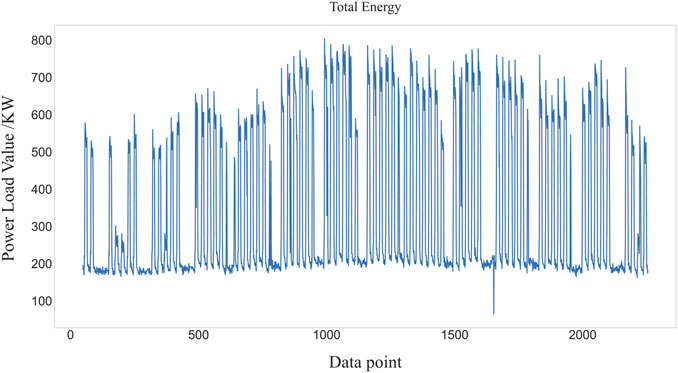
FIGURE 4. Original total energy series.

3.2 Comparison of Decomposition by EEMD and VMD

Figure 5A shows how EEMD decomposes the original load into 11 intrinsic mode functions (IMFs) and a residual, and Figure 5B shows the spectrum after passing the Fourier transform. Even with the improved EMD algorithm, the phenomenon of modal mixing is still evident. Modal mixing occurs when one modal component is decomposed into multiple components. In the figure, the frequency band of IMF4 overlaps with the frequency bands of IMF3 and IMF5. Modal mixing is a defect of the EEMD algorithm and leads to degradation of the model accuracy, so it is important to avoid this phenomenon.

FIGURE 5

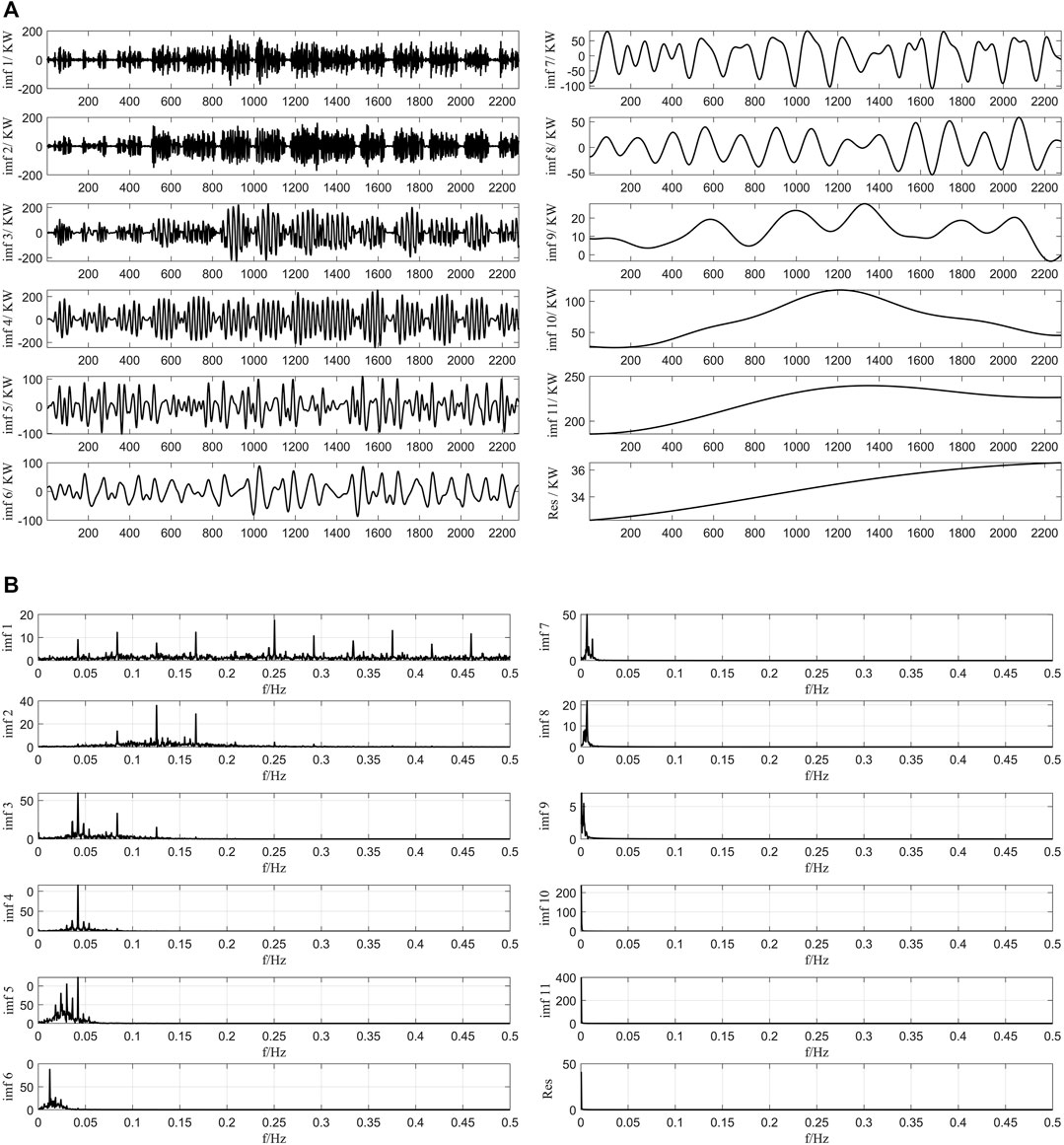
FIGURE 5. (A) The decomposition results of EEMD. (B) The decomposition spectrogram of EEMD.

The VMD algorithm solves the modal mixing problem inherent in the EEMD algorithm. In Figure 6A, the VMD decomposition results are shown for K = 4 and the penalty parameter a = 2000, which were determined in Section 2.1.2. u₁ is the lowest frequency component, u₂ is the medium frequency component and u₃ and u₄ are the highest frequency components. According to the additional analysis supplied by the spectrogram in Figure 6B, there is no overlap in the frequencies of the components, which indicates that the VMD algorithm solves the problem of modal mixing.

FIGURE 6

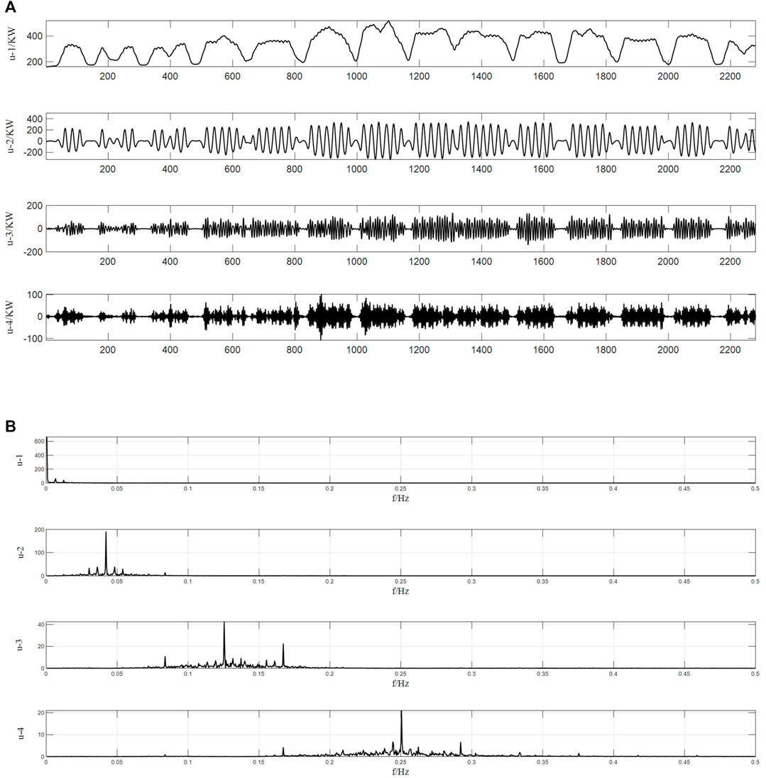
FIGURE 6. (A) The decomposition results of VMD. (B) The decomposition spectrogram of VMD.

In summary, both the EEMD and VMD algorithms are capable of handling volatile raw data, and both algorithms decompose the load into several stable components. The EEMD algorithm is an improved algorithm based on EMD, but it is limited due to the phenomenon of modal confusion. The VMD algorithm overcomes this shortcoming. The VMD algorithm can sufficiently decompose the raw load data to obtain more physically meaningful components and improve the accuracy of the model prediction.

3.3 Feature Selection

Building electricity consumption is influenced by climate and historical load. However, the raw data contains only meteorological factors. To fully consider the independence of each component and research the physical significance of each component, a set of feature matrices are established in this paper. The appropriate feature set is selected by the mRMR algorithm for input into the prediction model. The established feature matrices and their representations are shown in Table 1.

TABLE 1

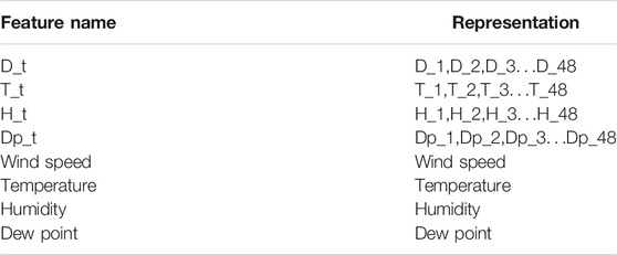
TABLE 1. Construction of feature matrix.

The time interval of the load data collected in this paper is 1 h. In Table 1, D_t represents the load point for the previous 48 h at time t. Similarly, T_t, H_t and Dp_t represent the temperature, humidity and dew point temperature, respectively, for the previous 48 h at time t. The wind speed, temperature, humidity and dew point are the meteorological characteristics of the dataset.

After establishing the feature matrix, each component of the decomposition is used as the target variable $y$, and $x_i$ is the data point in the feature matrix. The mRMR values are calculated according to Eq. 12 and the calculation results are sorted in descending order. The top 15 influencing factors are selected as the feature matrix of the input model. The final selection results are shown in Table 2.

TABLE 2

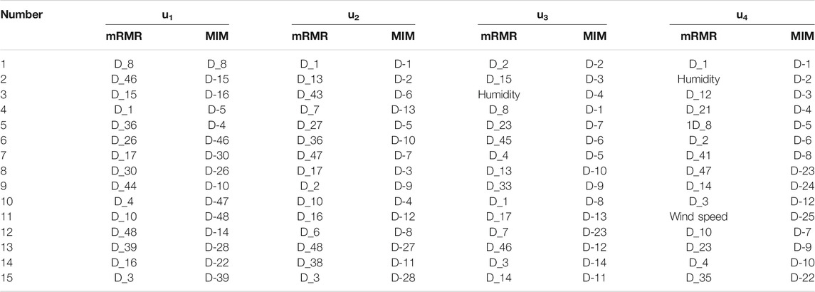
TABLE 2. Feature selection results.

To illustrate the superiority of the mRMR algorithm, mutual information maximization (MIM) (Novakovic et al., 2011) is used as a comparison in this paper. The MIM algorithm is based on the theory of mutual information, but unlike mRMR, the MIM algorithm only considers the correlation between features and target variables and does not consider the redundancy between features. The results of the MIM feature selection are shown in Table 2.

Consider u₁ and u₄ in Table 2 as an example. The low-frequency components u₁ and u₂ are mainly influenced by D_t, which indicates that the u₁ and u₂ components are influenced more heavily by the historical load of the past 48 h. It is further seen through Figure 6A that although both u₁ and u₂ are strongly influenced by historical loads, u₁ presents a load variation trend with a week as a period, while u₂ presents a load variation trend with a 24-h period. In contrast, the high-frequency components u₃ and u₄ are not only influenced by the historical load but also by the weather factor. Weather factors are usually seen as uncertainty factors. The influence of humidity on u₄ is ranked second among all the features. This explains why u₄ is more volatile than u₁: u₁ is mainly influenced by historical load and has a certain regularity, while u₄ is influenced by uncertainties such as humidity. Thus, u₄ is more irregular.

Table 3 shows that the results of the MIM feature selection method are similarly ranked, with the higher-ranked features all being historical loads at a given moment. This is especially apparent for the u₃ and u₄ components. The top five features selected using MIM have a high degree of overlap because the MIM algorithm only considers the maximum correlation between features and variables while ignoring the degree of redundancy between features. This is improved by using the mRMR algorithm. For u₃ and u₄, the feature overlap selected using the mRMR algorithm is not high, and features that are not considered by MIM, such as wind speed and humidity, are taken into account by the mRMR algorithm.

TABLE 3

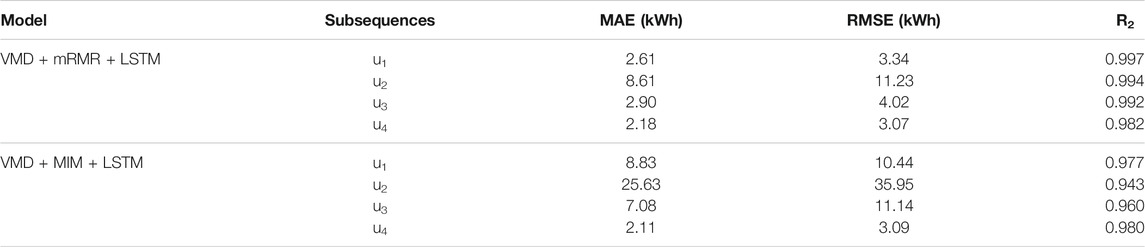
TABLE 3. VMD component prediction result.

In summary, the mRMR algorithm considers not only the correlation between features and target variables but also the degree of redundancy between features. The selected features can better reflect some characteristics of the modal components and reduce the dimensionality of the feature matrix.

3.3 Model Predictions

In this paper, the LSTM model is used for predictions. The training and test sets are divided for a total of 2,208 data points from June 1, 2017 to August 31, 2017. Of this data, 80% is used to build the model and 20% is used to check the validity of the established models.

The number of layers of the LSTM model serves to remember important information, and theoretically, more hidden layers give the model an improved nonlinear fitting ability and a better learning effect. However, increasing the number of layers consumes a considerable amount of computation time. According to the literature (Pan, 2018; Li et al., 2019), the number of implied layers generally does not exceed 3, so the number of implied layers in this paper has been determined to be 1.

The number of nodes in the hidden layer affects the performance of the model. If the number of nodes in the implicit layer is too small, less effective information is obtained in the prediction process. If the number of nodes in the implicit layer is too large, it may lead to a longer training time and overfitting problems. According to the literature (Xu et al., 2020), the number of nodes in the hidden layer can be determined by Eq. (26):

$l=\sqrt{m+n}+a(26)$

where $l$ is the number of nodes in the hidden layer, $m$ is the number of input nodes, $n$ is the number of output nodes, and $a$ is a constant from 1 to 10. By calculation, the number of nodes $l$ in the hidden layer is determined to be 8. The LSTM network is trained using the Adam optimization algorithm (Wang et al., 2019). By referring to relevant literature (Kong et al., 2019; Pei et al., 2020) and experimental measurements, the remaining parameters are set: The number of iterations of the neural network is set to 1,000, the learning rate is set to 0.01, and the expected error is set to 0.0004. The prediction results are shown in Figure 7 and Table 4.

FIGURE 7

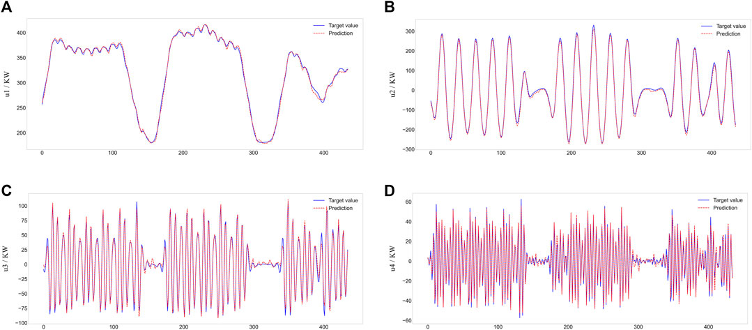
FIGURE 7. VMD component prediction figure.(A) u1, (B) u2, (C) u3, (D) u4.

TABLE 4

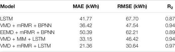
TABLE 4. Evaluation metrics of each model.

Figure 7 and Table 3 demonstrate that the integrated model proposed in this paper achieves better results for the prediction of each component. In general, the prediction results for the low and medium frequency components (u₁ and u₂, respectively) are better, with R² values of 0.997 and 0.994, respectively. The u₃ component also achieved a better prediction, having an R² value of 0.992. In contrast, the prediction results for the high-frequency component u₄ are slightly worse, with an R² value of only 0.982.

Table 3 also shows the prediction results for each component obtained using the MIM feature selection method. The R² values of the prediction results for all four components are lower than those obtained by the mRMR method, especially for the u₂ and u₃ components. The main reason for this result is because the MIM feature selection algorithm does not consider the redundancy among the features, which leads to a certain degree of repetitiveness of the selected features.

3.4 Model Comparison

The proposed model is compared and analysed alongside other models to verify its reliability. The other models are singular and include a model using EEMD decomposition (EEMD–mRMR–BPNN), a model using the MIM algorithm (VMD–MIM–LSTM) and a model using the BPNN algorithm (VMD–mRMR–BPNN). The prediction results and evaluation metrics of all models are shown in Figure 8 and Table 4.

FIGURE 8

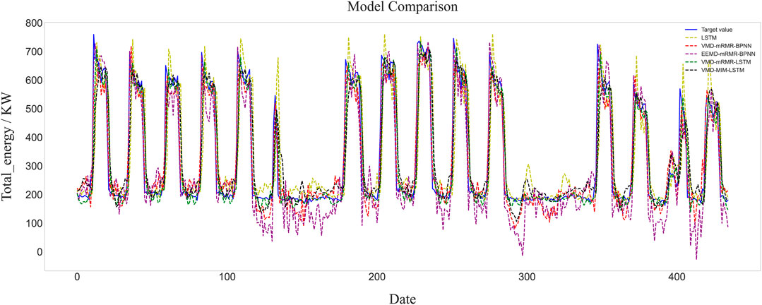
FIGURE 8. Prediction results of each model.

The predictions of the integrated model with the addition of the modal decomposition algorithm are more accurate compared to the single prediction model (LSTM), as shown in Figure 8. This indicates that the modal decomposition algorithm can indeed handle more complex data and improve the accuracy of the model. In addition, the prediction model proposed in this paper has the highest prediction accuracy among the four models.

According to the evaluation metrics analysis in Table 4, the prediction error of the single LSTM model is larger than the prediction error of the integrated model. This is mainly due to the instability of the load data and the limitations of the input features. The modal decomposition algorithm can decompose the fluctuating data into several stable IMFs, and the mRMR algorithm can select suitable features for the model. Thus, the prediction results of the integrated model are better than those of the single LSTM model. In addition, the integrated model using the VMD modal decomposition method (VMD–mRMR–BPNN) predicts better results than the integrated model using EEMD (EEMD–mRMR–BPNN). The R² is improved by 5.6% and the MAE and RMSE are reduced by 27.7 and 23.6%, respectively, because the VMD algorithm solves the problems of modal aliasing and elusive components.

Comparing the VMD–MIM–LSTM and VMD–mRMR–LSTM integrated models, the mRMR algorithm, which takes into account the redundancy between features, achieves better prediction accuracy for the feature selection algorithm. The R² is improved by 3.0%, the value of the MAE is reduced by 35.6% and the value of RMSE is reduced by 34.1%. This is because the mRMR algorithm takes into account the redundancy between features and can select the appropriate feature matrix for each IMF.

Comparing the VMD–mRMR–LSTM and VMD–mRMR–BPNN prediction models, the integrated model using LSTM outperforms the integrated model using BPNN. The R² of the LSTM integrated model is improved by 3.0%, the value of MAE is reduced by 41.4% and the value of RMSE is reduced by 35.5%. The power load series is a sample of power load variation over time, and the BPNN model has shortcomings in analysing these types of time series. For the time series, the LSTM model better mines the relationship between the data points. In brief, the model proposed in this paper has the highest prediction accuracy.

3.5 Model Robustness

The experimental results show that the hybrid model proposed in this paper has high prediction accuracy. In this section, the robustness of the hybrid model is analysed by varying the number of input feature parameters and the number of neurons in the hidden layer. For simplicity, the VMD-decomposed u₄ has been selected as the target dataset.

3.5.1 Number of Neurons in The Hidden Layers

In theory, with the increase of the number of neurons in the hidden layer and the more abstract features extracted by deep learning, the more accurate a time series will be, which is favourable for predictions (Zhang et al., 2020). Figure 9A shows the RMSE of the VMD–mRMR–LSTM and VMD–MIM–LSTM models when the number of neurons in the hidden layer is changed. When the number of hidden layer nodes is between 5 and 25, the RMSE shows a gradual decrease; when the number of hidden layer nodes is between 25 and 65, the RMSE has a large fluctuation; when the number of hidden layer nodes is between 65 and 100, the RMSE tends to be smooth, its value is mostly between 3 and 5 and the prediction error is relatively stable, which indicates that these two models are highly robust. In addition, the RMSE of VMD–mRMR–LSTM is lower than that of VMD–MIM–LSTM in most situations, which indicates that VMD–mRMR–LSTM has better prediction performance and more stable robustness.

FIGURE 9

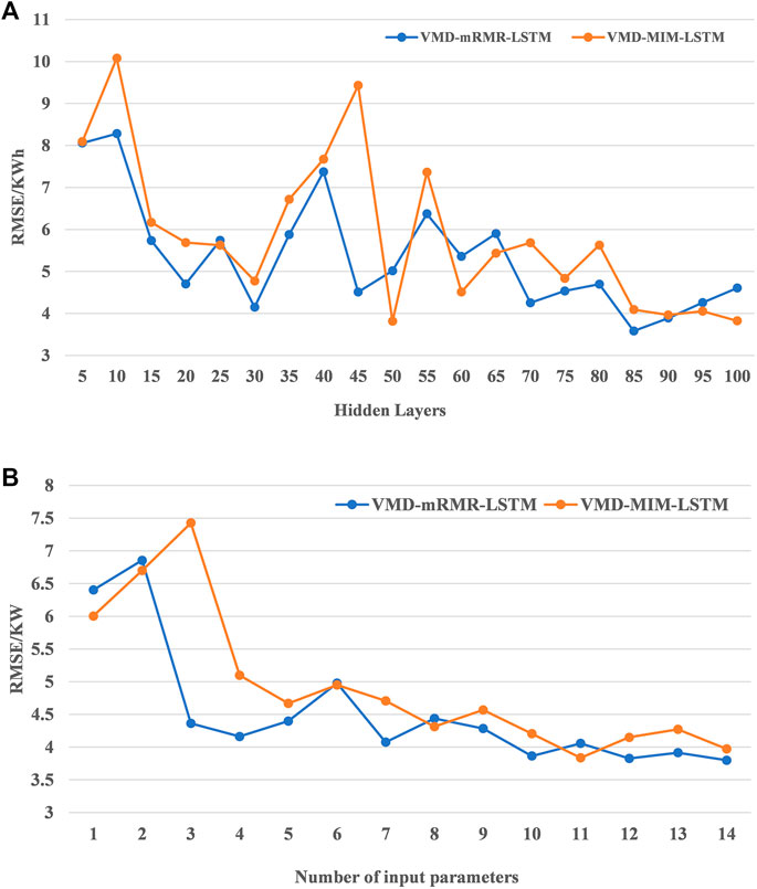
FIGURE 9. (A) Effect of the number of hidden layers on RMSE of u4. (B) Effect of the number of input parameters on RMSE of u4.

3.5.2 Number of Input Parameters

The redundancy between features is theoretically taken into account by the mRMR algorithm so that more input parameters lead to a better prediction performance of the model. However, too many feature parameters can increase the complexity of the model and increase the computing cost. Figure 9B illustrates the effect of the number of feature parameters on the accuracy of the model. When the number of input features is between 1 and 6, the RMSE of the models is decreasing and fluctuates. When the number of input features is between 6 and 15, the RMSE of both models decreases smoothly with values in the range of 3.5–4.5. The prediction error of the VMD–mRMR–LSTM model is smaller than that of the VMD–MIM–LSTM model. Therefore, the VMD–mRMR–LSTM model is more robust than the VMD–MIM–LSTM model when the number of input features is changed.

3.5.3 Effect of Input Data

To investigate the effect of different input data on the accuracy of the model, the training set in the 3.1 section is used as the raw data input to the hybrid model. Figure 10A shows the results of the training set decomposed by VMD. Comparing the decomposition results in Figure 6A, 10A, it can be seen that the trend of the training set is similar to the original data. Further comparing the spectrograms in Figure 6B, 10B, although the peak frequency of the training data set and the original data set is different, they appear at the same locations. The decomposition results of the training set are input into the hybrid model, and the prediction result is shown in Figure 11. The predicted values of MAE, RMSE, and R² are 30.96 kWh, 38.96 kWh, and 0.95, respectively. Compared with the results of decomposing the original data (VMD–mRMR–LSTM), the R² of the decomposed training dataset model (Training_Set-VMD–mRMR–LSTM) decreased by 2%, and the RMSE and MAE increased by 27 and 44.9%, respectively, indicating that the selection of the input data can have an impact on the accuracy of the model. Training_Set- VMD–mRMR–LSTM still has higher accuracy than the single LSTM model, and the R² improved by 7%, RMSE and MAE reduced by 42.4 and 25.9%, respectively. In conclusion, the use of training data as model input reduces the accuracy of the model, but the impact is small in general. Compared with a single model, the proposed hybrid model still has a greater superiority.

FIGURE 10

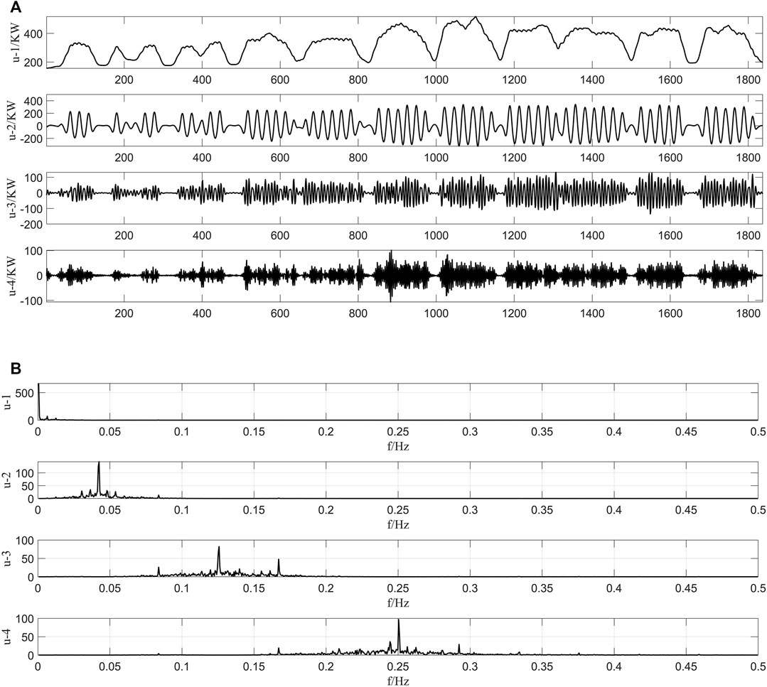
FIGURE 10. (A) The decomposition results of training set. (B) The decomposition spectrogram of training set.

FIGURE 11

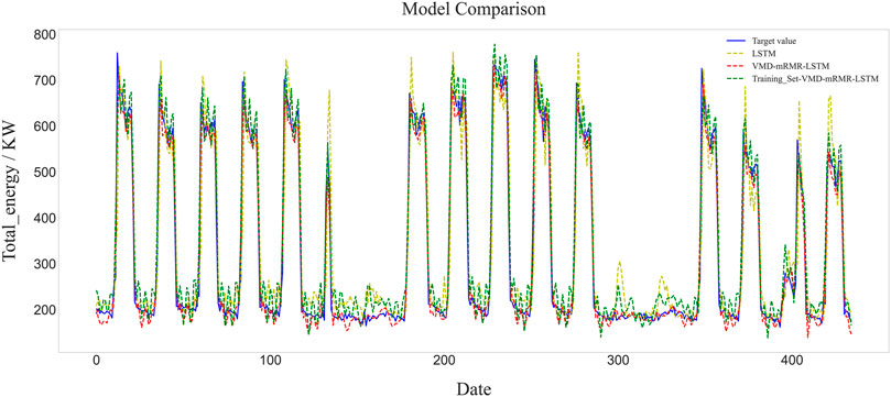
FIGURE 11. Prediction results of model with training set.

4 Conclusion

A hybrid short-term load forecasting model, namely VMD–mRMR–LSTM, was proposed in this paper. To solve the modal mixing problem presented by the EMD algorithm, the VMD algorithm was used, and the value of its decomposition number K was determined by the average instantaneous frequency. For feature selection, the mRMR algorithm was used to select the related feature by analysing the correlation between each component and feature as well as the redundancy between features. Finally, the LSTM model was used for the prediction model. The case study in this paper demonstrated the following:

1) Compared to single prediction models, hybrid models have higher accuracy and are more robust in the field of energy consumption prediction and have a broad application prospect for the short-term prediction of building energy consumption.

2) Using VMD to decompose the original sequence can have a better decomposition effect than when EEMD is used. Decomposition by VMD solves the problem of modal confusion so that the decomposed sequence is stable. The prediction results of the hybrid model using VMD are higher than those of the hybrid model using EEMD.

3) The mRMR algorithm can eliminate the redundancy between features and show the influencing factors of the modal components. The experimental results prove that the features selected by the mRMR algorithm have a higher prediction accuracy and better interpretability than those selected by MIM, which is supported by the value of R² increasing by 3%, the value of MAE decreasing by 35.6% and the value of RMSE decreasing by 34.1%.

4) The hybrid model proposed in this paper can achieve an R² value of 0.97, and its prediction results are higher than those of the single model (LSTM) and the general integrated model (VMD–MIM–LSTM). Therefore, the proposed VMD–mRMR–LSTM approach has a high potential for practical applications in energy systems, such as forecasting building energy consumption.

5) By varying the number of input feature parameters and the number of neurons in the hidden layer, the model is proven to have good robustness.

In this paper, all decomposed components were predicted using the LSTM model. However, since the frequency of each component varied, the LSTM may not have produced ideal results for each component. For example, in Table 3, the difference between the R² values of the u₁ and u₄ components for the VMD–mRMR–LSTM model was not negligible. Choosing appropriate prediction models for the different frequency components may lead to better results. We will conduct more research in this direction in the future.

Data Availability Statement

The data analyzed in this study is subject to the following licenses/restrictions: This study is applicable to the air conditioning cooling and heating load data of various building users. Requests to access these datasets should be directed to FQ, qianfanyue91@163.com.

Author Contributions

YR gave guidance on the framework and ideas of the paper. GW built the load forecasting model and compared it with conventional method. HM gave guidance on the framework and ideas of the paper. FQ gave guidance on the framework and ideas of the paper.

Funding

This research has been supported by the national key R&D project (No.2020YFD1100504-05).

Conflict of Interest

The authors declare that the research was conducted in the absence of any commercial or financial relationships that could be construed as a potential conflict of interest.

Publisher’s Note

All claims expressed in this article are solely those of the authors and do not necessarily represent those of their affiliated organizations, or those of the publisher, the editors and the reviewers. Any product that may be evaluated in this article, or claim that may be made by its manufacturer, is not guaranteed or endorsed by the publisher.

References

Amasyali, K., and El-Gohary, N. M. (2018). A Review of Data-Driven Building Energy Consumption Prediction Studies[J]. Renew. Sust. Energ. Rev. 81. doi:10.1016/j.rser.2017.04.095

CrossRef Full Text | Google Scholar

de Paiva, G. M., Pires Pimentel, Sergio., Pinheiro Alvarenga, Bernardo., Marra, E. G., Mussetta, Marco., and Leva, S. (2020). Multiple Site Intraday Solar Irradiance Forecasting by Machine Learning Algorithms: MGGP and MLP Neural Networks[J]. Energies 13 (11).

Google Scholar

Dong, B., Li, Z., Rahman, S. M. M., and Vega, R. (2016). A Hybrid Model Approach for Forecasting Future Residential Electricity Consumption. Energy and Buildings 117, 341–351. doi:10.1016/j.enbuild.2015.09.033

CrossRef Full Text | Google Scholar

Dragomiretskiy, K., and Zosso, D. (2014). Variational Mode Decomposition. IEEE Trans. Signal. Process. 62 (3), 531–544. doi:10.1109/TSP.2013.2288675

CrossRef Full Text | Google Scholar

Eom, J., Clarke, L., Kim, S. H., Kyle, P., and Patel, P. (2012). China's Building Energy Demand: Long-Term Implications from a Detailed Assessment. Energy 46 (1), 405–419. doi:10.1016/j.energy.2012.08.009

CrossRef Full Text | Google Scholar

Guo, Z., Zhao, W., Lu, H., and Wang, J. (2011). Multi-step Forecasting for Wind Speed Using a Modified EMD-Based Artificial Neural Network Model[J]. Renew. Energ. 37 (1).

Google Scholar

He, F., Zhou, J., Feng, Z-k., Liu, G., and Yang, Y. (2019). A Hybrid Short-Term Load Forecasting Model Based on Variational Mode Decomposition and Long Short-Term Memory Networks Considering Relevant Factors with Bayesian Optimization Algorithm[J]. Appl. Energ. 237. doi:10.1016/j.apenergy.2019.01.055

CrossRef Full Text | Google Scholar

He, Q., Wang, J., and Lu, H. (2018). A Hybrid System for Short-Term Wind Speed forecasting[J]. Kidlington, Oxford: Elsevier BV, 226.

Google Scholar

Hochreiter, S., and Schmidhuber, J. (1997). Long Short-Term Memory. Neural Comput. 9 (8), 1735–1780. doi:10.1162/neco.1997.9.8.1735

PubMed Abstract | CrossRef Full Text | Google Scholar

Hu, J., Wang, J., and Zeng, G. (2013). A Hybrid Forecasting Approach Applied to Wind Speed Time Series[J]. Renew. Energ. 60. doi:10.1016/j.renene.2013.05.012

CrossRef Full Text | Google Scholar

Huang Norden, E., Zheng, S., Long Steven, R., Wu, M. C., Shih Hsing, H., Zheng, Q., et al. (1998). The Empirical Mode Decomposition and the Hilbert Spectrum for Nonlinear and Non-stationary Time Series Analysis[J]. Proc. R. Soc. A: Math. Phys. Eng. Sci., 454.

Google Scholar

Kong, W., Dong, Z. Y., Jia, Y., David, J., Hill, Y. X., and Zhang, Y. (2019). Short-Term Residential Load Forecasting Based on LSTM Recurrent Neural Network.[J]. IEEE Trans. Smart Grid 10 (1).

CrossRef Full Text | Google Scholar

Li, C., Chen, Z. Y., and Liu, J. B. (2019). “Power Load Forecasting Based on the Combined Model of LSTM and XGBoost[C]//PRAI ’19,” in Proceedings of the 2019 the International Conference on Pattern Recognition and Artificial Intelligence (Wenzhou, China: ACM), 46–51.

Google Scholar

Li, C., Tao, Y., Ao, W., Yang, S., and Bai, Y. (2018). Improving Forecasting Accuracy of Daily enterprise Electricity Consumption Using a Random forest Based on Ensemble Empirical Mode Decomposition[J]. Energy 165. doi:10.1016/j.energy.2018.10.113

CrossRef Full Text | Google Scholar

Lin, Y ., and Peng, L. (2011). Combined Model Based on EMD-SVM for Short-Term Wind Power Prediction. Proc. CSEE 31, 102–108.

Google Scholar

Liu, H., Chen, C., Tian, H-Q., and Li, Y-F. (2012). A Hybrid Model for Wind Speed Prediction Using Empirical Mode Decomposition and Artificial Neural Networks[J]. Renew. Energ. 48. doi:10.1016/j.renene.2012.06.012

CrossRef Full Text | Google Scholar

Liu, H., Mi, X., and Li, Y. (2018). Smart Multi-step Deep Learning Model for Wind Speed Forecasting Based on Variational Mode Decomposition, Singular Spectrum Analysis, LSTM Network and ELM[J]. Energ. Convers. Manag. 159. doi:10.1016/j.enconman.2018.01.010

CrossRef Full Text | Google Scholar

Liu, M., Cao, Z., Zhang, J., Wang, L., Huang, C., and Luo, X. (2020). Short-term Wind Speed Forecasting Based on the Jaya-SVM Model[J]. Int. J. Electr. Power Energ. Syst. 121. doi:10.1016/j.ijepes.2020.106056

CrossRef Full Text | Google Scholar

Liu, Z., Wu, D., Liu, Y., Han, Z., Lun, L., Gao, J., et al. (2019). Accuracy Analyses and Model Comparison of Machine Learning Adopted in Building Energy Consumption Prediction[J]. Energy Exploration & Exploitation 37 (4). doi:10.1177/0144598718822400

CrossRef Full Text | Google Scholar

Marcello Anderson, F. B., Lima, P. C. M. C., Carneiro, T. C., Leite, J. R., Luiz, J., Neto, D. B., et al. (2017). Portfolio Theory Applied to Solar and Wind Resources Forecast[J]. IET Renew. Power Generation 11 (7). doi:10.1049/iet-rpg.2017.0006

CrossRef Full Text | Google Scholar

Muhammad, M., Francesco, G., Sonia, L., and Marco, M. (2020). Comparison of echo State Network and Feed-Forward Neural Networks in Electrical Load Forecasting for Demand Response Programs[J]. Mathematics Comput. Simulation, 184.

Google Scholar

Niu, H., Xu, K., and Wang, W. (2020). A Hybrid Stock price index Forecasting Model Based on Variational Mode Decomposition and LSTM network[J]. Dordrecht, Netherlands: Springer US.

Google Scholar

Novakovic, J., Strbac, P., and Bulatovic, D. (2011). Toward Optimal Feature Selection Using Ranking Methods and Classification Algorithms. Yugoslav J. Operation 21 (1), 119–135. doi:10.2298/YJOR1101119N

CrossRef Full Text | Google Scholar

Pan, B. (2018). Application of XGBoost Algorithm in Hourly PM2.5 Concentration Prediction[J]. IOP Conf. Series:Earth Environ. Sci., 113, 1–7.

CrossRef Full Text | Google Scholar

Pei, S., Qin, H., Yao, L., Liu, Y., Wang, C., and Zhou, J. (2020). Multi-Step Ahead Short-Term Load Forecasting Using Hybrid Feature Selection and Improved Long Short-Term Memory Network[J]. Energies 13 (16). doi:10.3390/en13164121

CrossRef Full Text | Google Scholar

Peng, H., Long, F., and Ding, C. (2005). Feature Selection Based on Mutual Information: Criteria of max-dependency, max-relevance, and Min-Redundancy. IEEE Trans. Pattern Anal. Mach Intell. 27 (8), 1226–1238. doi:10.1109/TPAMI.2005.159

PubMed Abstract | CrossRef Full Text | Google Scholar

Said, G. (2016). A New Ensemble Empirical Mode Decomposition (EEMD) Denoising Method for Seismic Signals[J]. Energ. Proced. 97.

Google Scholar

Sun, Z., Zhao, S., and Zhang, J. (2019). Short-Term Wind Power Forecasting on Multiple Scales Using VMD Decomposition, K-Means Clustering and LSTM Principal Computing[J]. IEEE Access 7. doi:10.1109/access.2019.2942040

CrossRef Full Text | Google Scholar

Sun, Z., Zhao, S., and Zhang, J. (2019). Short-Term Wind Power Forecasting on Multiple Scales Using VMD Decomposition, K-Means Clustering and LSTM Principal Computing. IEEE Access 7, 166917–166929. doi:10.1109/ACCESS.2019.2942040

CrossRef Full Text | Google Scholar

Wang, S., Sun, J., and Xu, Z. (2019). HyperAdam: A Learnable Task-Adaptive Adam for Network Training[J]. Proc. AAAI Conf. Artif. Intelligence 33. doi:10.1609/aaai.v33i01.33015297

CrossRef Full Text | Google Scholar

Wu, Y-X., Wu, Q-B., and Zhu, J-Q. (2018). Improved EEMD-Based Crude Oil price Forecasting Using LSTM Networks[J]. Physica A: Stat. Mech. its Appl., 516.

Google Scholar

Wu, Y. J. (2016). Research on Fault Diagnosis of Wind Turbine Transmission System Based on Variational Mode Decomposition. Dissertation. Beijing: North China Electric Power University.

Google Scholar

Wu, Z., and Huang, N. E. (2009). Ensemble Empirical Mode Decomposition: A Noise-Assisted Data Analysis Method[J]. Adv. Adaptive Data Anal. 1 (1).

Google Scholar

Xu, L., Zhou, C., Hu, Y., Li, G., and Xi, F. (2020). Energy Consumption Prediction of Chiller Based on Long Short-Term Memory [J]. Refrigeration & Air Conditioning 34 (06), 664–669.

Google Scholar

Zhang, M., Jiang, Z., and Kun, F. (2017). Research on Variational Mode Decomposition in Rolling Bearings Fault Diagnosis of the Multistage Centrifugal Pump[J]. Mech. Syst. Signal Process. 93. doi:10.1016/j.ymssp.2017.02.013

CrossRef Full Text | Google Scholar

Zhang, W., Liu, F., Zheng, X., and Li, Y . (2015). “A Hybrid EMD-SVM Based Short-Term Wind Power Forecasting Model,” in Proceedings of the 2015 IEEE PES Asia-Pacific Power and Energy Engineering Conference (APPEEC) (BrisbaneAustralia: QLD), 151–185. doi:10.1109/appeec.2015.7380872

CrossRef Full Text | Google Scholar

Zhang, Y., Yan, B., and Aasma, M. (2020). A Novel Deep Learning Framework: Prediction and Analysis of Financial Time Series Using CEEMD and LSTM[J]. Expert Syst. Appl. 159. doi:10.1016/j.eswa.2020.113609

CrossRef Full Text | Google Scholar

Zhu, D., Yan, D., and Wang, C. (2012). Comparison of Building Energy Simulation Software: DeST, EnergyPlus and DOE-2[J]. Building Sci. 28 (S2), 213–222.

Google Scholar