Forecasting of Steam Coal Price Based on Robust Regularized Kernel Regression and Empirical Mode Decomposition

Aiming at the problem of difficulties in modeling the nonlinear relation in the steam coal dataset, this article proposes a forecasting method for the price of steam coal based on robust regularized kernel regression and empirical mode decomposition. By selecting the polynomial kernel function, the robust loss function and L2 regular term to construct a robust regularized kernel regression model are used. The polynomial kernel function does not depend on the kernel parameters and can mine the global rules in the dataset so that improves the forecasting stability of the kernel model. This method maps the features to the high-dimensional space by using the polynomial kernel function to transform the nonlinear law in the original feature space into linear law in the high-dimensional space and helps learn the linear law in the high-dimensional feature space by using the linear model. The Huber loss function is selected to reduce the influence of abnormal noise in the dataset on the model performance, and the L2 regular term is used to reduce the risk of model overfitting. We use the combined model based on empirical mode decomposition (EMD) and auto regressive integrated moving average (ARIMA) model to compensate for the error of robust regularized kernel regression model, thus making up for the limitations of the single forecasting model. Finally, we use the steam coal dataset to verify the proposed model and such model has an optimal evaluation index value compared to other contrast models after the model performance is evaluated as per the evaluation index such as RMSE, MAE, and mean absolute percentage error.

Introduction

Accurate forecasting of the steam coal price can provide a certain basis for enterprises related to steam coal to formulate the procurement plan. The steam coal price indicates the general performance of supply and demand on the steam coal market. China is a big consumer of coal (Xiong and Xu, 2021; Wang and Du, 2020). Forecasting the steam coal price accurately can help in the analysis of the steam coal market, grasp the implied law in the steam coal market, and improve the steam coal market’s efficiency.

In recent years, many references have proposed many different methods for coal price forecasting. The time series model can mine the implicit law in the time series. Matyjaszek et al. removed the effect of abnormal fluctuations in prices on the forecasting model by using the transgenic time series (Matyjaszek et al., 2019). Ji et al. effectively improved the forecasting accuracy of the forecasting model by using the ARIMA model and neural network model (Ji et al., 2019). Wu et al. decomposed the price series into several components, used the ARIMA model and SBL model for coal price forecasting, and added up the forecasted values of all the components as final forecasting result. Compared to the contrast model adopted, this model can effectively improve the model forecasting precision (Wu et al., 2019). Chai et al. combined STL decomposition method with ETS model. The experimental results show that it has the best forecasting performance compared with benchmark models and neural network (Chai et al., 2021). It is difficult to learn the implicit nonlinearity law in the data by using the time series model, which is sensitive to the abnormal value in the data and only considers a single variable factor other than other influence factors.

A neural network model can learn the nonlinearity law in the data which is studied based on the interconnection between nerve cells. Alameer et al. effectively improved the forecasting accuracy of coal price based on LSTM model and DNN model (Alameer et al., 2020). Lu et al. adopted the full empirical mode to decompose and preprocess the original dataset, and then chose the radial basis function neural network model for model training and forecasting. The results show higher stability (Lu et al., 2020). Yang et al. adopted the improved whale optimization algorithm to optimize the decomposition and LSTM combined model based on the improved integration empirical model, which has a better model forecasting performance compared to other reference models (Yang et al., 2020). Zhang et al. decomposed the original data series by multi-resolution singular value decomposition method and forecasted the coal price by using MFO-optimized ELM model. Experimental results show the forecasting performance of the proposed model was superior to that of the contrast model (Zhang et al., 2019). However, the neural network model is a black box model which is difficult to interpret.

The steam coal market is a complex nonlinear system, containing influence factors such as economy, steam coal transportation, steam coal supply, and steam coal demand. The influence factors involve a wide range and many feature data and contain some noise data. This method improves the model interpretability by using linear model and reduces the adverse impact of noise data on the forecast model by using Huber loss function (Gupta et al., 2020). We use the kernel function to mine the implicit nonlinearity law in the steam coal data (Li and Li, 2019; Vu et al., 2019; Ye et al., 2021). The combined model can improve the model performance based on the advantages of the sub-model (Wang et al., 1210; Zhou et al., 2019; Wang et al., 2020a; Wang et al., 2020b; Qiao et al., 2021; Zhang et al., 2021). This method can decompose the forecasting error of the forecasting model into multiple modal components by using the EMD method (Yu et al., 2008; Xu et al., 2019; Wang and Wang, 2020; Xia and Wang, 2020), build the ARIMA model (Conejo et al., 2005; Karabiber and Xydis, 2019) for each modal component for forecasting, and add up the forecasted values of all the modal components to compensate error for the original forecasting model.

For the problem of difficulties in modeling the nonlinear relation in the steam coal dataset, this article proposes a forecast method for the price of steam coal based on robust regularized kernel regression and empirical mode decomposition. The second part introduces the used algorithm theory content; the third part states the data preprocessing steps, the selection of features, and the whole process of model training and forecasting; the fourth part shows the model comparison and experimental results; and the fifth part contains conclusion and prospect.

Methodology

Huber–Ridge Model

The Huber function (Huber et al., 1992) has great robustness, which can effectively reduce the negative influence of abnormal data on model performance. The Huber loss function is shown in Eq. 1:

${\varphi }_{\text{hub}}\left(u\right)=\{\begin{array}{cc}{u}^2& \left|u\right|\le M\\ M\left(2\left|u\right|-M\right)& \left|u\right|>M\end{array},(1)$

where $u$ is the residual value and M is the threshold value of the Huber function. The Huber function imposes the punishment which is larger than the threshold value residual to effectively lower the influence of abnormal sample points on the model training.

The Ridge model is added with L2 penalty term based on the objective function of the linear regression model. The objective function of the model is shown in Eq. 2:

$\underset{\text{ω}}{\min }\frac{1}{2}\Vert X\omega -Y{\Vert }_2^2+{\alpha }_{l2}\Vert \omega {\Vert }_2^2,(2)$

where $X$ refers to the set of feature parameters, $\omega$ refers to the weight coefficient vector, $Y$ refers to the forecasted target quantity, $\Vert \omega {\Vert }_2^2$ refers to the L2 penalty term, and ${\alpha }_{l2}$ refers to the regular coefficient.

L2 regular term compresses the feature weight value adversely to the model forecasting and makes it approximate to 0 in order to reduce the impact of features with low correlation. When the regular coefficient of ${\alpha }_{l2}$ is large, the L2 regular term makes more parameters’ weight in the parameter weight vector approximate to 0 to screen out main features and mitigate the degree of model overfitting to some extent.

The Huber loss function and L2 regular term are combined to construct the Huber–Ridge model (Owen, 2006), improving the model robustness and lowering the overfitting risk. Its objective function is shown in Eq. 3:

${\widehat{w}}_j={\mathrm{argmin}}_w \left({\varphi }_{\mathrm{hub}}\left(u\right)+\frac{\lambda }{2}{\displaystyle \sum _{j=1}^k{\left(w_j\right)}^2}\right).(3)$

Polynomial Kernel Huber–Ridge Model

The T.M. Cover theorem (Cover, 1965) points out that the data in the high-dimensional space can show the linearity law more easily. The kernel function maps the vector of low-dimensional feature space to the high-dimensional feature space, and transforms the nonlinearity law in the low-dimensional feature space into linearity law in the high-dimensional space to learn the linearity law in the high-dimensional space by using the linear model and indirectly learn the nonlinearity law in the original feature space based on the model. Due to the high-dimensional feature space having high dimensionality, the dimension disaster may happen if the model is directly used for fitting in the high-dimensional space. The introduced kernel function can effectively solve the above problem, and the kernel function can represent inner product value in the high-dimensional space with the inner product value in the low-dimensional space. Thus, it can avoid the inner product calculation in the high-dimensional space and greatly reduce the calculation of the model.

The regular risk functions have a unified expression mode (Schölkopf et al., 2001), as shown in Eq. 4:

$f\left(x\right)={\displaystyle \sum _{i=1}^n{w}_{i}k\left(x,x_i\right)+b}.(4)$

The kernel function is introduced to the Huber–Ridge model (Jianke Zhu et al., 2008). Thus, the model can learn the implicit nonlinearity law in the data. The objective function of Huber–Ridge kernel model is shown in Eq. 6:

$u=y_i-f\left(x\right),(5)$

where $y_i$ is the actual value, $f\left(x\right)$ is the forecasting value, and $u$ is the forecasting error

${\mathrm{\varphi }}_{\text{hub}}\left(y_i,f\left(x\right)\right)=\{\begin{array}{cc}M\left(2u-M\right)& A_1=\left\{x\text{|}u>M\right\}\\ u^2& A_2=\left\{x\text{|}-M\le u\le M\right\}\\ -M\left(2u-M\right)A_3& A_3=\left\{x\right|u>M\}\end{array},(6)$

${\widehat{w}}_j={\mathrm{argmin}}_{\mathrm{w}} {\displaystyle \sum _{j=1}^n{\mathrm{\varphi }}_{\mathrm{hub}}}\left(y_i,{\displaystyle \sum _{i=1}^{n}k}\left(x_i,x_j\right)w_j+b\right)+\lambda {\displaystyle \sum _{i,j=1}^n{w}_i{w}_{j}k\left(x_i,x_j\right)},(7)$

$T={\mathrm{argmin}}_{\mathrm{w}}{\displaystyle \sum _{i=1}^n{\mathrm{\varphi }}_{\text{hub}}}\left(y,{\displaystyle \sum _{i=1}^n{k}_i^T}w+b·I\right)+\lambda w^{T}Kw.(8)$

Eqs. 9–12 can be obtained, respectively, by getting the partial derivative of $w$ and $b$:

$\frac{\partial \text{T}}{\partial w}=2\left(\lambda Kw+K{I}^{0}Kw+Kq\right)=0,(9)$

$\mathrm{q}=-I^{0}y+me+b·I^0,(10)$

${\mathrm{e}}_i=\{\begin{array}{c}1\\ 0\\ -1\end{array}\begin{array}{c}{x}_i\in A_1\\ x_i\in A_2\\ x_i\in A_3\end{array},(11)$

$\frac{\partial T}{\partial b}=2\left(I^0\mathrm{Kw}+q\right)=0,(12)$

where $I^0$ is a diagonal matrix of shape (n, n), the values of its elements in the A domain are 1, and the remaining values are 0.

The basic Newton method is used to iteratively update $w$ and $b$, as shown in Eq. 13:

$\left[\begin{array}{c}{w}^{\prime }\\ b^{\prime }\end{array}\right]=\left[\begin{array}{c}w\\ b\end{array}\right]-\text{γ}{H}^{-1}\nabla ,(13)$

where ${\text{H}}^{-1}$ is the first derivative of the gradient matrix as shown in Eq. 14, $\text{γ}$ is the length of the step, usually with a value of 1, and $\nabla$ is a Hessen matrix as shown in Eq. 15:

$H^{-1}=\frac{1}{2}{\left[\begin{array}{cc}\lambda K+K{I}^{0}K& I^{0}K\\ K{I}^0& I^0\end{array}\right]}^{-1},(14)$

$\nabla =2\left[\begin{array}{c}\lambda Kw+K{I}^{0}Kw+Kq\\ I^{0}Kw+q\end{array}\right].(15)$

Simplify Eq. 13 to obtain the final computational equation of objective function of the kernel Huber–Ridge model, as shown in Eq. 16:

$\left[\begin{array}{c}{w}^{\prime }\\ b^{\prime }\end{array}\right]=\left[\begin{array}{c}0\\ b\end{array}\right]+{\left[\begin{array}{cc}\lambda I+I^{0}K& 1\\ 1& 0\end{array}\right]}^{-1}\left[\begin{array}{c}q\\ 0\end{array}\right].(16)$

The polynomial kernel is a commonly used kernel function, and the polynomial kernel function is shown in Eq. 17:

$\mathbf{K}\left(\mathbf{x},\mathbf{x}\right)={\left(\mathbf{x}·\mathbf{x}+1\right)}^d,(17)$

where $\mathbf{x}=\left(x_1,x_2,\cdots ,x_n\right)$ is the feature vector and d is the kernel parameter. The polynomial kernel function (17) is substituted into Eq. 16 to obtain the final computational equation of polynomial kernel Huber–Ridge model objective function.

EMD Model

The empirical mode decomposition is a signal decomposition technology and decomposes the original signal into a series of components which are the intrinsic mode functions. The empirical mode decomposition is often used to handle the time series data and decomposes the original time series into a series of different components to explore the implicit law in the time series data.

The intrinsic mode function should meet the two conditions below:

1. In the data interval, difference between numbers of extreme points and zero points is at most one.

2. The average value of the upper envelope and the lower envelope is zero.

The EMD model is adaptive and can decompose the original series for a time series data without the number of components specified till the standard of stopping decomposition is met. The relationship between the original series and the decomposed components is shown in Eq. 18:

$\mathrm{X}\left(\text{t}\right)={\displaystyle \sum _{i=1}^{n}im{f}_i+r},(18)$

where $\text{X}\left(\text{t}\right)$ refers to the original time series, ${\displaystyle \sum }_{i=1}^{n}im{f}_i$ refers to the sum of the components, and r refers to the residual. When the residual series is a monotonic function, the decomposition stopped.

The decomposition step of empirical mode decomposition is shown as follows:

STEP 1: Identify all the maximum points and minimum points in the time series, and fit the upper envelope ${\text{e}}_{\text{u}}$ and the lower envelope ${\text{e}}_{\text{l}}$ by using the cubic spline finite difference method according to maximum points and minimum points.

STEP 2: Calculate the average value of the upper envelope ${\text{e}}_{\text{u}}$ and the lower envelope ${\text{e}}_{\text{l}}$, and obtain the mean envelope ${\mathrm{e}}_{\mathrm{mean}}$$\left({\mathrm{e}}_{\mathrm{mean}}=\frac{{\mathrm{e}}_{\mathrm{u}}+{\mathrm{e}}_{\mathrm{l}}}{2}\right)$.

STEP 3: Calculate the difference between the original series $X\left(t\right)$ and the mean envelope${\text{ e}}_{\text{mean}}$, and obtain the intermediate time series$({\text{ e}}_{\text{i}}$$=\mathrm{X}\left(\mathrm{t}\right)-{\mathrm{e}}_{\mathrm{mean}})$.

STEP 4: Judge whether the intermediate time series ${\text{e}}_{\text{i}}$ can be an intrinsic mode function according to the constraint condition of intrinsic mode functions. If satisfied, the intermediate time series shall be used as the ${\text{imf}}_{\text{i}}$ component. If unsatisfied, such intermediate time series shall be used as the basis to execute the steps 1–4.

STEP 5: Subtract the component ${\text{imf}}_{\text{i}}$ from the original time series $X\left(t\right)$ and execute the steps 1–4 again. If the standard of stopping decomposition is satisfied, the decomposition process will end.

ARIMA Model

The autoregressive integrated moving average (ARIMA) model is defined in Eq. 19:

$y^t={\phi }_1{y}^{t-1}+{\phi }_2{y}^{t-2}+\cdots +{\phi }_p{y}^{t-p}+{\epsilon }^t-{\theta }_1{\epsilon }^{t-1}-{\theta }_2{\epsilon }^{t-2}-\cdots -{\theta }_q{\epsilon }^{t-q}+{\theta }_0,(19)$

where ${\text{y}}^{\text{t}}$ and ${\epsilon }^t$ indicate the actual value and residual value at the time point t, respectively, and $\phi =\left({\phi }_1,{\phi }_2,\cdots ,{\phi }_p\right)$ and $\theta =\left({\theta }_1,{\theta }_2,\cdots ,{\theta }_q\right)$ refer to the weight vectors. p and q are the model orders. The historical time series data and historical white noise error data of the variable are used to forecast the current value.

The prerequisite of using ARIMA model is to use stationary data. The non-stationary data can be handled by combining the autoregressive integrated moving average (ARIMA) model and different methods (Gilbert, 2005). The ARIMA model has three parameters, (p, d, q), in which d refers to the differential order of the data series.

Evaluation Indexes

The model performance is evaluated by the mean absolute error (MAE) and the definition of MAE is shown in Eq. 20:

$\mathrm{MAE}=\frac{1}{n}{\displaystyle \sum _{i=1}^n\left|y_i-{\widehat{y}}_i\right|}.(20)$

The root-mean-square error (RMSE) is used for model performance assessment and the definition of RMSE is shown in Eq. 21:

$\mathrm{RMSE}=\sqrt{\frac{1}{n}{\displaystyle \sum _{i=1}^n{\left(y_i-{\widehat{y}}_i\right)}^2}}.(21)$

The mean absolute percentage error (MAPE) is used for model performance assessment and the definition of MAPE is shown in Eq. 22:

$\mathrm{MAPE}=\frac{1}{n}{\displaystyle \sum _{i=1}^n\left|\frac{y_i-{\widehat{y}}_i}{y_i}\right|},(22)$

where n is the number of samples in the set verified, ${\widehat{\text{y}}}_i$ is the forecasted value of the model, and $y_i$ is the true value. The closer the MAE, RMSE, and MAPE values are to 0, the better the model performance will be.

The Training and Forecasting Process of Polynomial Kernel Huber–Ridge–EMD–ARIMA Model

The training and forecasting process for the forecast framework of polynomial kernel Huber–Ridge–EMD–ARIMA model (PK–Huber–Ridge–EMD–ARIMA) proposed is shown in Figure 1. Its process steps are as follows.

FIGURE 1

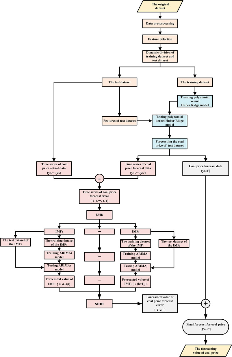
FIGURE 1. Flowchart for training and forecasting of the PK–Huber–Ridge–EMD–ARIMA model.

STEP 1: Data preprocessing and feature selection: Screen the correlation features according to Pearson correlation coefficient and Spearman correlation coefficient after the data preprocessing and divide training dataset and test dataset.

STEP 2: Model training: The model parameter $\text{M},{\alpha }_{l2}$, and training dataset are input to the polynomial kernel Huber–Ridge for model training.

STEP 3: Model forecasting: The test dataset is input to the trained polynomial kernel Huber–Ridge model. The model outputs the time series $\left\{y_1^{\prime },\cdots ,y_k^{\prime },y_{k+1}^{\prime }\right\}$ of coal price forecasting data.

STEP 4: Forecast the forecasting error of steam coal price at the next time point: The forecasting error series $\left\{{\epsilon }_1,\cdots {\epsilon }_k\right\}$ of coal price is input to the EMD model, and the EMD model outputs j modal components ($IM{F}_1,\cdots ,IM{F}_j$). Each modal component is subject to training and forecasting by the ARIMA model; the ARIMA model $(ARIM{A}_1,\cdots ,ARIM{A}_j)$ corresponding to each modal component outputs the coal price forecasting error (${\epsilon }_{k+1}^1,\cdots ,{\epsilon }_{k+1}^j$) of each modal component at the next time point, respectively. The (${\epsilon }_{k+1}^1,\cdots ,{\epsilon }_{k+1}^j$) series accumulation is conducted, and the accumulation result $\left\{{\text{ε}}_{\text{k}+1}^{\text{'}}\right\}$ is used as the forecasted value of the coal price forecasting error at a time point k+1.

STEP 5: Obtain the final forecasted value of steam coal price at the next time point: The forecasted value $\left\{{\text{ε}}_{\text{k}+1}^{\text{'}}\right\}$ of coal price forecasting error at the time point k+1 is used for $\left\{y_{k+1}^{\text{'}}\right\}$ correction of the forecasted value of coal price at a time point k+1. The forecasted value $\left\{y_{k+1}^{\text{'}\text{'}}\right\}$ of coal price after correction is used as the forecasted value of coal price at the final time point k+1.

Empirical Study

Data Description

Qinhuangdao steam coal price data that are 4500-kilocalorie, 5000-kilocalorie, and 5500-kilocalorie steam coal exit price data of Qinhuangdao Port from Jan. 2017 to Jul. 2021, are used for experimental study. The sampling is conducted once a week, which is the weekly frequency data.

Data Preprocessing

The original data about steam coal price and its features have the disadvantage of missing value and inconsistent data time sampling frequency; so, such original data shall be pre-processed and the data processed can be brought into the model for model training and forecasting.

The data preprocessing step is shown as follows:

1. Unify the data sampling frequency: The data input to the model have the features of one-to-one relationship between coal feature data and coal price, that is, the sampling frequency of coal feature data and coal price data is the same. When the sampling frequency of the original coal price data and related feature data is inconsistent, such original data shall be operated at the unified data sampling frequency; the frequency of the data higher than the specified sampling frequency shall be reduced and the frequency of the data lower than the specified sampling frequency shall be raised. The daily frequency data are reduced to weekly frequency data. The quarterly and monthly data are raised to the weekly data and the missing value arises after the low-frequency data are raised to the high-frequency data. The raised data are processed by ascending order as per the date, and then the missing value is filled up by linear difference filling.

2. Fill up the missing value: There are some missing values and non-numerical parts in the original coal data which need to be filled up to better utilize the dataset. The missing part in the data is filled up by linear difference, and the non-numerical part is deleted and then the missing part deleted is filled up by linear difference. The equation of missing value between filling points $({\text{x}}_0,{\text{y}}_0)$ and $({\text{x}}_{\text{k}},{\text{y}}_{\text{k}})$ is shown in Eq. 23:

$\text{ϕ}\left(x\right)=\frac{x-x_k}{x_0-x_k}{y}_0+\frac{x-x_0}{x_k-x_0}{y}_k.(23)$

3. Standardize the dataset: There is a dimensional difference between different types of data. To avoid the dimensional error and lower the model performance, the standardized equation is used to transform the data distribution into standard distribution with the mean value of 0 and variance of 1. The standardized equation is shown as follows:

$\{\begin{array}{c}{x}_{ki}=\frac{X_{ki}-\overline{X_i}}{{\sigma }_i}\\ {\sigma }_i=\frac{{\left(X_{1i}-\overline{X_i}\right)}^2+{\left(X_{2i}-\overline{X_i}\right)}^2+\dots +{\left(X_{ni}-\overline{X_i}\right)}^2}{n}\end{array}.(24)$

After transformation as per Eq. 24, the distribution of original feature data is transformed into a standard normal distribution with the mean value of 0 and variance of 1. $x_{ki}$ indicates the kth numerical value of the ith feature index. $\overline{X_i}$ indicates the mean value of the ith feature index data, ${\sigma }_i$ indicates the standard deviation of the ith feature index, and $n$ indicates the sample size of the ith feature index.

4) Divide training dataset and test dataset: The training dataset and test dataset are not fixed, but they change dynamically. In the energy market, the influencing factors of energy indicators change with time (Liang et al., 2019). The coal data and related feature data at the time point within the sliding window of k width are used as the training dataset for training the price forecasting model. The price forecasting model outputs the forecasted coal price at a time point according to the coal-related feature data after sliding the window. The corresponding original price data and relevant feature data are used as the test dataset to verify the model forecasting performance. The dynamic division of the training dataset and test dataset progresses over time, as shown in Figure 2.

FIGURE 2

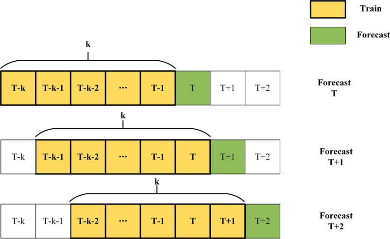
FIGURE 2. Dynamic division of training dataset and test dataset.

Feature Selection

Selecting comprehensive and relevant features can greatly improve the performance of the forecasting model. All feature data are presented as a data matrix, and the optimal feature variable is chosen according to the feature type and feature optimal time interval.

Feature type: The coal price pertains to many factors; there are many factors influencing coal market price, and the main influence factors cover coal supply coal consumption, coal transportation, and economic factor. The feature indexes chosen are shown in Table 1.

TABLE 1

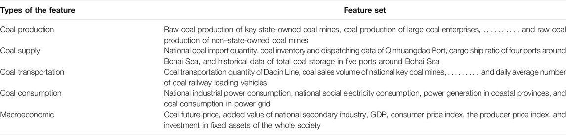
TABLE 1. Selection of steam coal feature data.

There are many initial feature indexes, so the feature screening needs to be performed. The feature variable at the same time point as the forecasted target variable does not necessarily have the highest correlation, and it is necessary to find out the optimal time interval, that is, optimal delay order, for each feature variable. The optimal delay linear feature and the optimal delay nonlinear relevant features are screened as per Pearson correlation coefficient and Spearman correlation coefficient.

The value range of Pearson correlation coefficient ${\text{r}}_{\text{p}}$ Spearman and correlation coefficient $r_s$ is [-1, 1]. The closer the absolute value of ${\text{r}}_{\text{p}}$ and $r_s$ is to 1, the stronger the correlation will be; the closer the absolute value of ${\text{r}}_{\text{p}}$ and $r_s$ is to 0, the weaker the correlation will be.

Given the corresponding threshold values of the Pearson correlation coefficient and Spearman correlation coefficient are ${\text{r}}_{\text{mp}}$ and ${\text{r}}_{\text{sp}}$, respectively, the feature indexes whose correlation coefficient exceeds the threshold value ${\text{r}}_{\text{mp}}$ and ${\text{r}}_{\text{sp}}$ are screened. Given the maximum delay order of the feature is $dela{y}_{max}$, the parameter setting is shown in Table 2.

TABLE 2

TABLE 2. Parameters setting of the feature selection process.

The chosen feature variables and steam coal price are input to the forecasting model mentioned, and the model outputs the steam coal price at the next time point. Table 3 and Table 4 show the selection of the optimal delay feature variable when forecasting the steam coal price on Jul. 6, 2021. The feature variable selected as per this method changes over time.

TABLE 3

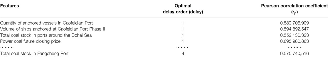
TABLE 3. Linear features with optimal delay.

TABLE 4

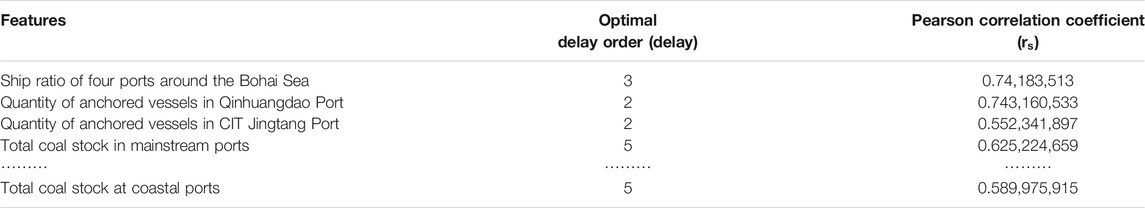
TABLE 4. Nonlinear features with optimal delay.

Experiment Result

In this article, Lasso, Ridge, Huber–Ridge, PK–Huber–Ridge, and PK–Huber–Ridge–EMD–ARIMA models are used for comparison. One-step forecasting is used for empirical test. Qinhuangdao thermal coal data and feature data at the first 120 time points are used as the data variables of the forecasting model, and the forecasting model outputs the thermal coal price data at the 121st time point.

The set values of hyperparameters of Lasso, Ridge, Huber–Ridge, PK–Huber–Ridge, and PK–Huber–Ridge–EMD–ARIMA models are shown in Table 5.Here, ${\text{α}}_{\text{l}1}$ is the coefficient of L1 regular term; ${\text{α}}_{\text{l}2}$ is the coefficient of L2 regular term; M is the threshold of Huber loss function; ${\text{d}}_{\text{k}}$ is the kernel parameter of the polynomial kernel and represents the order of the polynomial; p is the autoregressive order of ARIMA model; $d_a$ represents the difference order; and q represents the moving average order. BIC criterion (Burnham and Anderson, 2004) is used to select the optimal ARIMA model hyperparameters p, $d_a$, and q.

TABLE 5

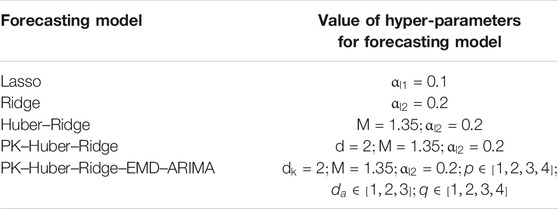
TABLE 5. Value of hyper-parameters for five different models.

The forecasting model is used to forecast 4500-kilocalorie steam coal price data (Dataset 1), 5000-kilocalorie steam coal price data (Dataset 2), and 5500-kilocalorie steam coal price data (Dataset 3) of Qinhuangdao Port from March 17, 2020 to July 6, 2021. Table 6 and Figure 3 and Figure 4 and Figure 5 show the evaluation index results of the forecasting model.

TABLE 6

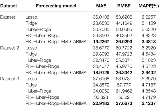
TABLE 6. Evaluation index value of forecasting results of five forecasting models.

FIGURE 3

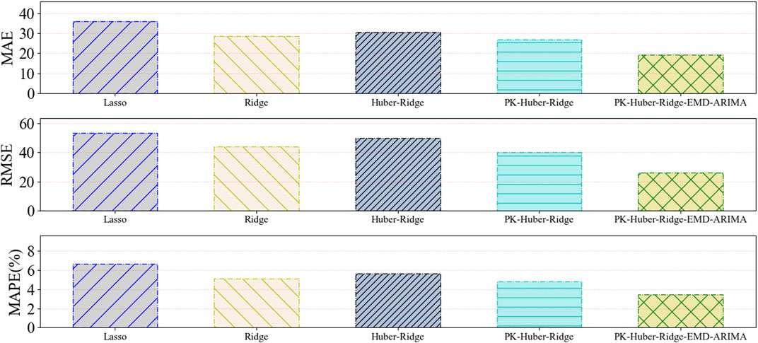
FIGURE 3. A histogram of the predictive evaluation index values based on dataset 1 for five types of forecasting models.

FIGURE 4

FIGURE 4. A histogram of the predictive evaluation index values based on dataset 2 for five types of forecasting models.

FIGURE 5

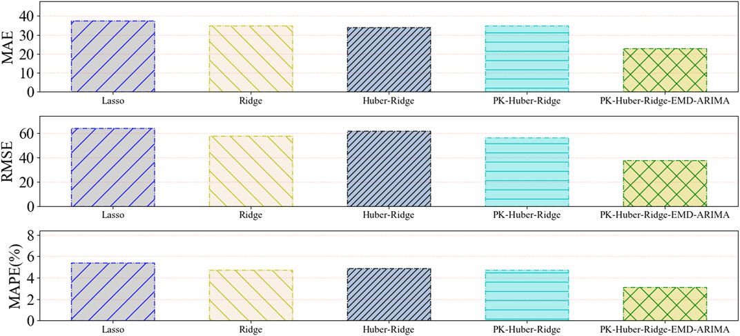
FIGURE 5. A histogram of the predictive evaluation index values based on dataset 3 for five types of forecasting models.

Through the comparison of the experimental results of five thermal coal price forecasting models, the following conclusions can be obtained.

Compared with the single model, the proposed combination model has a better forecasting performance. In dataset 1, dataset 2, and dataset 3 experiments, the forecasting performance of PK–Huber–Ridge–EMD–ARIMA model is better than the Lasso model, Ridge model and Huber–Ridge model, and PK–Huber–Ridge model. The thermal coal price dataset is complex, and the forecasting performance of a single forecasting model is very limited. The combination model can better deal with complex datasets. PK–Huber–Ridge–EMD–ARIMA model adopts the method of decomposition integration and time series forecasting model to compensate for the error of single model. We consider the residual error rule of model forecasting to complement the hidden rules that the original single model does not learn.

Compared with the ordinary model, the robust kernel function model has better performance. In dataset 1, dataset 2, and dataset 3 experiments, the forecasting performance of PK–Huber–Ridge–EMD–ARIMA model is better than the Lasso model, Ridge model, and Huber–Ridge model. Thermal coal dataset has nonlinear law. PK–Huber–Ridge–EMD–ARIMA model uses polynomial kernel function to map nonlinear features into high-dimensional space, so that the linear model can learn the nonlinear law in the original feature space, so as to further improve the forecasting performance of the forecast model.

Result and Discussion

For the nonlinearity law in the steam coal dataset and limitations of the single forecasting model, this article proposes the forecast method for the price of steam coal based on robust regularized kernel regression and empirical mode decomposition. The robust regularized kernel regression model learns the nonlinearity law in the original data by using the kernel function. This model selects the Huber loss function to enhance the robustness of the forecasting model. We select the L2 regular term to lower the risk of model overfitting. The combined model based on EMD and ARIMA is used for error compensation against the Huber–Ridge polynomial kernel model, further improving the forecasting performance of the forecasting model. Compared to Lasso, Ridge, Huber–Ridge, and PK–Huber–Ridge, the proposed forecasting model (PK–Huber–Ridge–EMD–ARIMA) has the minimum value of MAE, RMSE, and MAPE.

The influence factors of steam coal price are complex which are easily affected by national policies. How to quantify policy factors and input them into the forecasting model for model training and model forecasting is the next work.

Data Availability Statement

The data analyzed in this study are subject to the following licenses/restrictions: The data used to support the findings of this study are currently under embargo, while the research findings are commercialized. Requests to access these datasets should be directed to tmz@csust.edu.cn.

Author Contributions

All authors listed have made a substantial, direct, and intellectual contribution to the work and approved it for publication.

Funding

This work was supported in part by the National Natural Science Foundation of China (Grant Nos. 62173050 and 61403046), the Natural Science Foundation of Hunan Province, China (Grant No. 2019JJ40304), Changsha University of Science and Technology “The Double First Class University Plan” International Cooperation and Development Project in Scientific Research in 2018 (Grant No. 2018IC14), the Research Foundation of the Education Bureau of Hunan Province (Grant No.19K007), Hunan Provincial Department of Transportation 2018 Science and Technology Progress and Innovation Plan Project (Grant No. 201843), Energy Conservation and Emission Reduction Hunan University Student Innovation and Entrepreneurship Education Center, Innovative Team of Key Technologies of Energy Conservation, Emission Reduction and Intelligent Control for Power-Generating Equipment and System, CSUST, Hubei Superior and Distinctive Discipline Group of Mechatronics and Automobiles(XKQ2021003 and XKQ2021010), Major Fund Project of Technical Innovation in Hubei (Grant No. 2017AAA133), and Guangxi Key Laboratory of Trusted Software (No.201728), Graduate Scientific Research Innovation Project of Changsha University of Science and Technology (No. 2021-89).

Conflict of Interest

DX was employed by China Datang Corporation Ltd., Beijing, China.

JY was employed by Hunan Datang Xianyi Technology Co., Ltd., Changsha, China.

The remaining authors declare that the research was conducted in the absence of any commercial or financial relationships that could be construed as a potential conflict of interest.

Publisher’s Note

All claims expressed in this article are solely those of the authors and do not necessarily represent those of their affiliated organizations, or those of the publisher, the editors and the reviewers. Any product that may be evaluated in this article, or claim that may be made by its manufacturer, is not guaranteed or endorsed by the publisher.

References

Alameer, Z., Fathalla, A., Li, K., Ye, H., and Jianhua, Z. Multistep-ahead Forecasting of Coal Prices Using a Hybrid Deep Learning Model. Resour. Pol. 65, 2020.

Google Scholar

Burnham, K. P., and Anderson, D. R. (2004). Multimodel Inference. Sociological Methods Res. 33 (2), 261–304. doi:10.1177/0049124104268644

CrossRef Full Text | Google Scholar

Chai, J., Zhao, C., Hu, Y., and Zhang, Z. G. (2021). Structural Analysis and Forecast of Gold price Returns. J. Manag. Sci. Eng. 6 (2), 135–145. doi:10.1016/j.jmse.2021.02.011

CrossRef Full Text | Google Scholar

Conejo, A. J., Plazas, M. A., Espinola, R., and Molina, A. B. (2005). Day-ahead Electricity price Forecasting Using the Wavelet Transform and ARIMA Models. IEEE Trans. Power Syst. 20 (2), 1035–1042. doi:10.1109/tpwrs.2005.846054

CrossRef Full Text | Google Scholar

Cover, T. M. (1965). Geometrical and Statistical Properties of Systems of Linear Inequalities with Applications in Pattern Recognition. IEEE Trans. Electron. Comput. EC-14 (3), 326–334. doi:10.1109/pgec.1965.264137

CrossRef Full Text | Google Scholar

Gilbert, K. (2005). An ARIMA Supply Chain Model. Manag. Sci. 51 (2), 305–310. doi:10.1287/mnsc.1040.0308

CrossRef Full Text | Google Scholar

Gupta, D., Hazarika, B. B., and Berlin, M. (2020). Robust Regularized Extreme Learning Machine with Asymmetric Huber Loss Function. Neural Comput. Applic 32 (16), 12971–12998. doi:10.1007/s00521-020-04741-w

CrossRef Full Text | Google Scholar

Huber, P. J. (1992). “Robust Estimation of a Location Parameter,” in Breakthroughs in Statistics: Methodology and Distribution. Editors S. Kotz, and N. L. Johnson (New York, NY: Springer New York), 492–518. doi:10.1007/978-1-4612-4380-9_35

CrossRef Full Text | Google Scholar

Ye, J., He, L., and Jin, H. (2021). A Denoising Carbon price Forecasting Method Based on the Integration of Kernel Independent Component Analysis and Least Squares Support Vector Regression. Neurocomputing 434, 67–79.

CrossRef Full Text | Google Scholar

Ji, L., Zou, Y., He, K., and Zhu, B. (2019). Carbon Futures price Forecasting Based with ARIMA-CNN-LSTM Model. Proced. Comp. Sci. 162, 33–38. doi:10.1016/j.procs.2019.11.254

CrossRef Full Text | Google Scholar

Jianke Zhu, J., Hoi, S., and Lyu, M. R. T. (2008). Robust Regularized Kernel Regression. IEEE Trans. Syst. Man. Cybern. B 38 (6), 1639–1644. doi:10.1109/tsmcb.2008.927279

PubMed Abstract | CrossRef Full Text | Google Scholar

Karabiber, O. A., and Xydis, G. (2019). Electricity Price Forecasting in the Danish Day-Ahead Market Using the TBATS, ANN and ARIMA Methods. Energies 12 (5). doi:10.3390/en12050928

CrossRef Full Text | Google Scholar

Li, Y., and Li, Z. (2019). Forecasting of Coal Demand in China Based on Support Vector Machine Optimized by the Improved Gravitational Search Algorithm. Energies 12 (12). doi:10.3390/en12122249

CrossRef Full Text | Google Scholar

Liang, T., Chai, J., Zhang, Y. J., and Zhang, Z. G. (2019). Refined Analysis and Prediction of Natural Gas Consumption in China. J. Manag. Sci. Eng. 4 (2), 91–104. doi:10.1016/j.jmse.2019.07.001

CrossRef Full Text | Google Scholar

Lu, H., Ma, X., Huang, K., and Azimi, M. Carbon Trading Volume and price Forecasting in China Using Multiple Machine Learning Models. J. Clean. Prod. 249, 2020.

Google Scholar

Matyjaszek, M., Riesgo Fernández, P., Krzemień, A., Wodarski, K., and Fidalgo Valverde, G. (2019). Forecasting Coking Coal Prices by Means of ARIMA Models and Neural Networks, Considering the Transgenic Time Series Theory. Resour. Pol. 61, 283–292. doi:10.1016/j.resourpol.2019.02.017

CrossRef Full Text | Google Scholar

Owen, A. B. (2006). A Robust Hybrid of Lasso and ridge Regression. Contemp. Math. 443, 59–72.

Google Scholar

Qiao, W., Liu, W., and Liu, E. A Combination Model Based on Wavelet Transform for Predicting the Difference between Monthly Natural Gas Production and Consumption of U.S. Energy 235, 2021.

Google Scholar

Schölkopf, B., Herbrich, R., and Smola, A. J. (2001).A Generalized Representer Theorem. In Computational Learning Theory. Berlin, Heidelberg, 416–426. doi:10.1007/3-540-44581-1_27

CrossRef Full Text | Google Scholar

Vu, D. H., Muttaqi, K. M., Agalgaonkar, A. P., and Bouzerdoum, A. (2019). Short-Term Forecasting of Electricity Spot Prices Containing Random Spikes Using a Time-Varying Autoregressive Model Combined with Kernel Regression. IEEE Trans. Ind. Inf. 15 (9), 5378–5388. doi:10.1109/tii.2019.2911700

CrossRef Full Text | Google Scholar

Wang, B., and Wang, J. Energy Futures and Spots Prices Forecasting by Hybrid SW-GRU with EMD and Error Evaluation. Energ. Econ., 90, 2020.

Google Scholar

Wang, J., Cao, J., Yuan, S., and Cheng, M. Short-term Forecasting of Natural Gas Prices by Using a Novel Hybrid Method Based on a Combination of the CEEMDAN-SE-And the PSO-ALS-Optimized GRU Network. Energy 233, 121082.

Google Scholar

Wang, J., Lei, C., and Guo, M. Daily Natural Gas price Forecasting by a Weighted Hybrid Data-Driven Model. J. Pet. Sci. Eng. 192, 2020.

Google Scholar

Wang, J., Zhou, H., Hong, T., Li, X., and Wang, S. A Multi-Granularity Heterogeneous Combination Approach to Crude Oil price Forecasting. Energ. Econ. 91, 2020.

Google Scholar

Wang, K., and Du, F. (2020). Coal-gas Compound Dynamic Disasters in China: A Review. Process Saf. Environ. Prot. 133, 1–17. doi:10.1016/j.psep.2019.10.006

CrossRef Full Text | Google Scholar

Wu, J., Chen, Y., Zhou, T., and Li, T. (2019). An Adaptive Hybrid Learning Paradigm Integrating CEEMD, ARIMA and SBL for Crude Oil Price Forecasting. Energies 12 (7). doi:10.3390/en12071239

CrossRef Full Text | Google Scholar

Xia, C., and Wang, Z. Drivers Analysis and Empirical Mode Decomposition Based Forecasting of Energy Consumption Structure. J. Clean. Prod. 254, 2020.

Google Scholar

Xiong, J., and Xu, D. (2021). Relationship between Energy Consumption, Economic Growth and Environmental Pollution in China. Environ. Res. 194.

CrossRef Full Text | Google Scholar

Xu, W., Hu, H., and Yang, W. (2019). Energy Time Series Forecasting Based on Empirical Mode Decomposition and FRBF-AR Model. IEEE Access 7, 36540–36548. doi:10.1109/access.2019.2902510

CrossRef Full Text | Google Scholar

Yang, S., Chen, D., Li, S., and Wang, W. (2020). Carbon price Forecasting Based on Modified Ensemble Empirical Mode Decomposition and Long Short-Term Memory Optimized by Improved Whale Optimization Algorithm. Sci. Total Environ. 716, 137117. doi:10.1016/j.scitotenv.2020.137117

PubMed Abstract | CrossRef Full Text | Google Scholar

Yu, L., Wang, S., and Lai, K. K. (2008). Forecasting Crude Oil price with an EMD-Based Neural Network Ensemble Learning Paradigm. Energ. Econ. 30 (5), 2623–2635. doi:10.1016/j.eneco.2008.05.003

CrossRef Full Text | Google Scholar

Zhang, H., Yang, Y., Zhang, Y., He, Z., Yuan, W., Yang, Y., et al. (2021). A Combined Model Based on SSA, Neural Networks, and LSSVM for Short-Term Electric Load and price Forecasting. Neural Comput. Applic 33 (2), 773–788. doi:10.1007/s00521-020-05113-0

CrossRef Full Text | Google Scholar

Zhang, X., Zhang, C., and Wei, Z. (2019). Carbon Price Forecasting Based on Multi-Resolution Singular Value Decomposition and Extreme Learning Machine Optimized by the Moth–Flame Optimization Algorithm Considering Energy and Economic Factors. Energies 12 (22). doi:10.3390/en12224283

CrossRef Full Text | Google Scholar

Zhou, J., Huo, X., Xu, X., and Li, Y. (2019). Forecasting the Carbon Price Using Extreme-Point Symmetric Mode Decomposition and Extreme Learning Machine Optimized by the Grey Wolf Optimizer Algorithm. Energies 12 (5). doi:10.3390/en12050950

CrossRef Full Text | Google Scholar