A Comparison of Muon Flux Models at Sea Level for Muon Imaging and Low Background Experiments

Cosmic-ray muons are a type of natural radiation with high energy and a strong penetration ability. The flux distribution of such particles at sea level is a key problem in many areas, especially in the field of muon imaging and low background experiments. This paper summarizes the existing models to describe sea-level muon flux distributions. According to different means used, four parametric analytical models and one Monte Carlo model, which is referred to as CRY, are selected as typical sea-level muon flux distribution models. Then, the theoretical values of sea-level muon fluxes given by these models are compared with the experimental sea-level muon differential flux data with kinetic energy values in the range of 1–1,000 GeV in the directions of zenith angles 0° and 75°. The goodness of fit of these models to the experimental data was quantitatively calculated by Pearson’s chi-square test. The results of the comparison show that the commonly used Gaisser model overestimates the muon flux in the low-energy region, while the muon flux given by the Monte Carlo model CRY at the large zenith angle of 75° is significantly lower than that of the experimental data. The muon flux distribution given by the other three parametric analytical models is consistent with the experimental data. The results indicate that the original Gaisser model is invalid in the low energy range, and CRY apparently deviates at large zenith angles. These two models can be substituted with the muon flux models given by Gaisser/Tang, Bugaev/Reyna, and Smith and Duller/Chatzidakis according to actual experimental conditions.

Introduction

Cosmic-ray muons are an essential component of natural radiation at sea level and are produced by the interactions of primary cosmic rays at the top of the Earth’s atmosphere. The specific characteristics of cosmic-ray muons—high energy, strong penetration ability, natural existence, and harmlessness to the structure of objects—make them a promising tool in imaging. According to the different effects of the interaction of muons with matter, there are two types of muon imaging: muon radiography and muon tomography. Muon radiography, which can realize the nondestructive imaging of the internal structure of large-scale objects (such as volcanoes, pyramids, underground caves, etc.), uses the principle that the energy loss of muons is related to the density and thickness of the material through which the muons penetrate. Muon tomography uses the scattering angle of cosmic-ray muons, which is related to the atomic number of materials, to image materials with high atomic numbers such as nuclear materials. With the development of detection technology in recent years, muon imaging has rapidly developed and achieved many promising research results. For example, Kunihiro Morishima et al. discovered a large-scale hidden void in the Khufu pyramid in 2017 using muon radiography (Morishima et al., 2017). From 2014 to 2015, Hirofumi Fujii et al. used muon radiography to image the internal structure of the Fukushima nuclear power plant after the Fukushima accident (Fujii et al., 2020), which provided strong technical support for accident handling. In contrast to the general imaging technique of X/γ-ray imaging, both muon radiography and muon tomography utilize naturally existing cosmic-ray muons as the particle source to image. Since sea-level cosmic-ray muons are the decay products of air showers induced by the hadronic interaction between primary cosmic rays and the atmosphere, their angles and energy distributions are affected by the altitude, latitude and other factors. Therefore, one of the key problems of muon imaging is the knowledge of the energy spectrum and angular distribution of cosmic-ray muons; the accuracy of these components directly affects the imaging result.

In addition to muon imaging, the study of sea-level muon flux models can help solve some key problems in low background experiments. Because of the strong penetration ability and high flux of cosmic ray muons at sea level, muons and muon-induced secondary particles account for an appreciable part of environment background, which will disturb the detection of dark matter, neutrinos and other low background experiments. To precisely simulate and assess the background caused by cosmic-ray muons, an accurate understanding of the energy spectrum and angular distribution of sea-level muons is crucial. Many attempts have been made on it. For example, Zi-yi Guo et al. measured the muon flux in China Jinping Underground Laboratory in order to provide a reference for passive and active shielding designs for future underground neutrino experiments, and the experiment result agreed well with simulation data (Guo et al., 2020). In addition, in-vivo radioisotope measurements are also sensitive to background radiation, and J. Turko et al. simulated the cosmic ray muon background at the Carlsbad Environmental Monitoring and Research Center to quantify its contribution to the total environmental background. They made further investigation on modifications to improve the detector system based on the simulation results (Turko et al., 2020).

Muon fluxes at sea level play a key role in solving many problems in different research fields. However, at present, many models are used to describe the distribution of cosmic-ray muon fluxes. Therefore, it is necessary to compare these models to provide guidance for muon imaging and other applications. In this paper, we summarize the major models of sea-level muon flux and compare them with experimental data. In Muon Flux Model at Sea Level, several representative and easy-to-use models to describe the sea-level muon flux are presented, and their characteristics are introduced. Comparison With Experimental Data compares these models by contrasting model predictions with experimental data. The last section presents the summary and discussion.

Muon Flux Model at Sea Level

The distribution of sea-level muons is usually described by their differential fluxes. As shown in Eq. 1, the differential flux of muons can be defined as the number of muons dN falling in unit area dS per unit energy dE per unit solid angle dΩ and per unit time dt.

$\mathit{\Phi }=\frac{{\text{d}}^{4}N}{\text{d}S\text{d}E\text{d}t\text{d}\Omega }\left({\text{GeV}}^{-1}{\text{cm}}^{-2}{\text{s}}^{-1}{\text{sr}}^{-1}\right)(1)$

The definition of $\text{Ф}$ in Eq. 1 indicates that the sea-level differential flux depends on the energy and direction of a muon. The direction of a muon can be determined by its zenith angle and azimuth angle. As shown in Figure 1, the xOy plane is at sea level, and the z-axis is perpendicular to sea level. Zenith angle θ is defined as the angle between the z-axis and the direction of a muon, and the azimuth angle φ is defined as the angle between the projection of a muon’s direction on the xOy plane and x-axis.

FIGURE 1

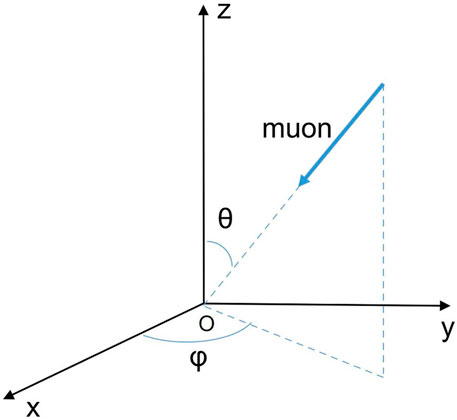
FIGURE 1. Direction of a muon at sea level.

Although the distribution of muons at sea level with respect to the azimuth φ is affected by factors such as geomagnetic fields and solar modulations, the effects are relatively small, so it can be approximately considered that the distribution of muons with respect to φ is uniform. Since the thickness of the atmosphere penetrated by muons increases with θ, the dependence of muon flux on θ is prominent, especially in the low-energy range, where the muon flux is approximately proportional to ${\text{cos}}^2\theta$. Therefore, the distribution of sea-level muon fluxes mainly refers to the distribution of the differential muon flux with respect to kinetic energy $E_0$ and θ.

There are two approaches to obtain the distribution of sea-level muon flux: 1) one way is to derive a parametric analytical model by fitting an empirical model to the measured data of sea-level muon flux; 2) the other way is to use Monte Carlo methods to simulate the process of primary cosmic ray incident into the Earth’s atmosphere and subsequent atmospheric cascade shower and finally obtain the distribution of muon flux at sea level. Previous studies have been performed following these two directions, and various feasible models have been proposed. The following will be introduced from these two aspects.

Parametric Analytical Model

The parametric analytical model is derived from an empirical model and based on the physical process of muon production and transport or a simple parametric model with no physical meaning. Parameters in these models are usually optimized by fitting to experimental data. Many attempts have been made to give a parametric analytical model that can calculate the differential muon flux at a given ($E_0,\theta$). Here, several commonly used models are presented as follows:

Gaisser Model

This model was proposed by Gaisser in 1990 and concerns the production of muons from the two-body decay of pions and kaons (Gaisser, 1990). When the muon energy $E_{\mu }\gg {\mathit{ϵ}}_{\mu }$, where ${\mathit{ϵ}}_{\mu }$ = 1.0 GeV is the critical energy for atmospheric muons, muon decay and energy loss in the atmosphere can be neglected. Therefore, the analytical form of this model is given as follows:

${\mathit{\Phi }}_G\left(E_0,\theta \right)=A_G{E}_0^{-\gamma }\left(\frac{1}{1+\widehat{E_0}cos\theta /{\epsilon }^{\prime }}+\frac{B_G}{1+\widehat{E_0}cos\theta /{{\epsilon }^{\prime }}_K}\right)(2)$

Here, $\widehat{{\mathit{E}}_0}$ is the muon energy at the top of the atmosphere; ${\mathit{E}}_0$ is the muon energy at sea level; at high energy, ${\mathit{E}}_0\approx \widehat{{\mathit{E}}_0}$; θ is the zenith angle of the muon; ${\mathit{A}}_{\text{G}}$ = 0.14 is a scale factor; γ = 2.7 is the index of energy spectrum; ${\mathit{ϵ}}_{\text{π}}^{\text{'}}=(115/1.1)\text{ GeV}$ and ${\mathit{ϵ}}_{\text{K}}^{\text{'}}=(810/1.1)\text{ GeV}$ are the critical energies of pion and kaon, respectively, divided by a factor related to their attenuation length; ${\mathit{B}}_{\text{G}}=0.054$ is a factor to evaluate the ratio of muons produced from kaon decay to muons produced from pion decay.

However, while deriving the model, the curvature of the atmosphere was ignored. This ignorance led to some deviation in the estimation of atmospheric thickness. Thus the attenuation of through-going muons was overestimated. With increasing zenith angles, this deviation will become increasingly significant. As a result, this model is only suitable for zenith angles θ < 60°, which are not very large.

Gaisser/Tang Model

Tang et al. found that the original Gaisser model ignored the curvature of the atmosphere, which caused deviations at large zenith angles, and overestimated muon flux within the energy range of $E_0<100/\text{cos}\theta .$ Therefore, they proposed a segmented modification formula based on Eq. 2, which can be written as follows (Tang et al., 2006):

${\mathit{\Phi }}_T\left(E_0,\theta \right)=A_T\times 0.14E_0^{-\gamma }\left(\frac{1}{1+1.1\widehat{E_0}cos{\theta }^{\text{*}}/115}+\frac{0.054}{1+1.1\widehat{E_0}cos{\theta }^{\text{*}}/810}+r_c\right)(3)$

$E_0$, $\widehat{E_0}$, and $\theta$ in Eq. 3 have identical meaning to those in Eq. 2. $A_T$ in Eq. 3 is also a scale parameter, and $\text{cos}{\theta }^{\text{*}}=\sqrt{\frac{x^2+p_1^2+p_2{x}^{p_3}+p_4{x}^{p_5}}{1+p_1^2+p_2+p_4}}$ is the modified $\text{cos}\theta$ that considers the atmospheric curvature, where $x\equiv \text{cos}\theta$, $p_1=0.102573$, $p_2=-0.068287$, $p_3=0.958633$, $p_4=0.0407253$, and $p_5=0.817285$.$r_c$ in Eq. 3 is the proportion of prompt muons produced by the decay of charmed particles.

The modification steps are as follows:

① If $E_0>100/\text{cos}{\theta }^{\text{*}}\text{GeV}$, let $A_T=1$ and $r_c=0$;

② While $1/\text{cos}{\theta }^{\text{*}}\text{GeV}<E_0<100/\text{cos}{\theta }^{\text{*}}\text{GeV}$, let $\widehat{E_0}=E_0+\text{Δ}$, where $\text{Δ}=2.06\times {10}^{-3}(\frac{950}{\text{cos}{\theta }^{\text{*}}}-90)$, $r_c={10}^{-4}$, $A_T=1.1{\left(\frac{90\sqrt{\text{cos}\theta -0.001}}{1030}\right)}^{4.5/\left(E_0\text{cos}{\theta }^{\text{*}}\right)}$;

③ For $E_0<1/\text{cos}{\theta }^{\text{*}}\text{GeV}$, substitute $E_0$ with $\frac{3E_0-7\text{sec}{\theta }^{\text{*}}}{10}$ based on the modifications in ① and ②.

Bugaev/Reyna Model

This model was first proposed by Bugaev in 1998. In addition to the energy loss of the muons produced by the two-body decay of pions and kaons, the muons produced by the three-body decay of kaons were also considered. Since the model aims to describe only the vertical differential flux of muons, the atmospheric curvature has no effect on the transport of muons and can be excluded. The model is expressed in the form of a fitting formula (Bugaev et al., 1998).

${\mathit{\Phi }}_B\left(p\right)=A_B{p}^{-(a_3{y}^3+a_2{y}^2+a_{1}y+a_0)}(4)$

In Eq. 4, p is the muon momentum at sea level, and $y={\log }_{10}p$; $A_B$, $a_0$, $a_1$, $a_2$, and $a_3$ are fitting parameters. The parameter values are adjusted with different momentum p ranges, as shown in Table 1.

TABLE 1

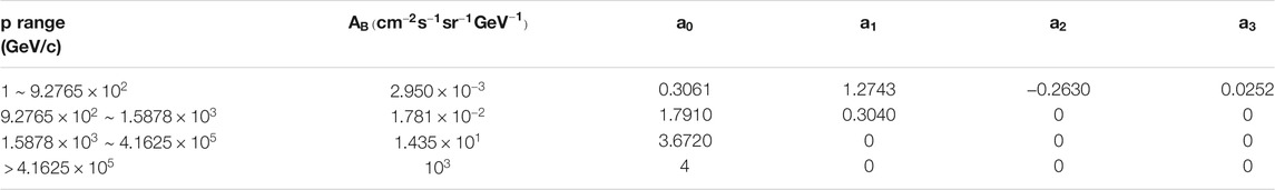
TABLE 1. Different parameter values for different p ranges (Tang et al., 2006).

In 2006, Reyna proposed a model that extends the model of vertical sea-level differential flux to all zenith angles based on Bugaev’s original model. Reyna analysed and processed several groups of experimental data of sea-level muons. The finding was that when the flux was multiplied by${\text{ cos}}^3\left(\theta \right)$, the distributions of the experimental data with different $p\text{cos}\theta$ were similar. Therefore, Reyna proposed an improved model based on Bugaev model, which replaces momentum p in Eq. 4 with $p\text{cos}\theta$ and multiplies it by a coefficient of ${\text{cos}}^3\left(\theta \right)$, as shown in Eq. 5 (Reyna, 2006).

${\mathit{\Phi }}_R\left(p,\theta \right)=\mathrm{c}\mathrm{o}{\mathrm{s}}^3\left(\theta \right){\mathit{\Phi }}_B\left(p\text{cos}\theta \right)(5)$

The parameters in Eq. 5 are also replaced with $A_B=0.00253,a_0=0.2455$, $a_1=1.288$, $a_2=-0.2555$, and $a_3=0.0209$. Reyna’s improved model is suggested for a momentum range of $1\text{GeV}\le p\le 2000/\text{cos}\theta \text{GeV}$ and a zenith angle range of $0°\le \theta \le 90°$.

Smith and Duller/Chatzidakis Model

This model was first developed by Smith and Duller in 1959. The model assumes that all muons come from pion decay. It is assumed that pions obtain a fixed proportion of energy from the primary cosmic ray that produces them and maintain the same velocity direction. Considering the absorption and decay of pions in the transport process, the pion transport equation is obtained. According to this equation, a similar assumption is used to derive the differential flux formula of muons at sea level, as shown in Eq. 6 (Smith and Duller, 1959):

${\mathit{\Phi }}_S(E_0,\theta )=\frac{A{E}_{\pi }{\left(E_0\right)}^{-\gamma }{P}_{\mu }{\lambda }_{\pi }b{j}_{\pi }}{E_{\pi }\left(E_0\right)\cos \theta +b{j}_{\pi }}(6)$

where $E_{\pi }$ is the energy of the pion that produced the muon, and $P_{\mu }$ is the probability for muons to reach sea level, which are calculated by Eqs 7, 8, respectively:

$E_{\pi }=\left[1/r\right]\left[E_0+a{y}_0\left(\sec \theta -0.100\right)\right](7)$

$P_{\mu }={\left\{0.100\text{cos}\theta \cdot \left(1-\frac{a(y_0\sec \theta -100)}{r{E}_{\pi }}\right)\right\}}^{B_{\mu }/\left[\left(r{E}_{\pi }+100a\right)\cos \theta \right]}(8)$

$B_{\mu }$ is calculates as follows:

$B_{\mu }=\frac{b_{\mu }{m}_{\mu }{y}_{0}c}{{\tau }_{{\mu }_0}{\rho }_0}.(9)$

In 2015, Chatzidakis et al. modified the parameters in the model by fitting them to experimental data (Chatzidakis et al., 2015). The modified parameters are listed in Table 2:

TABLE 2

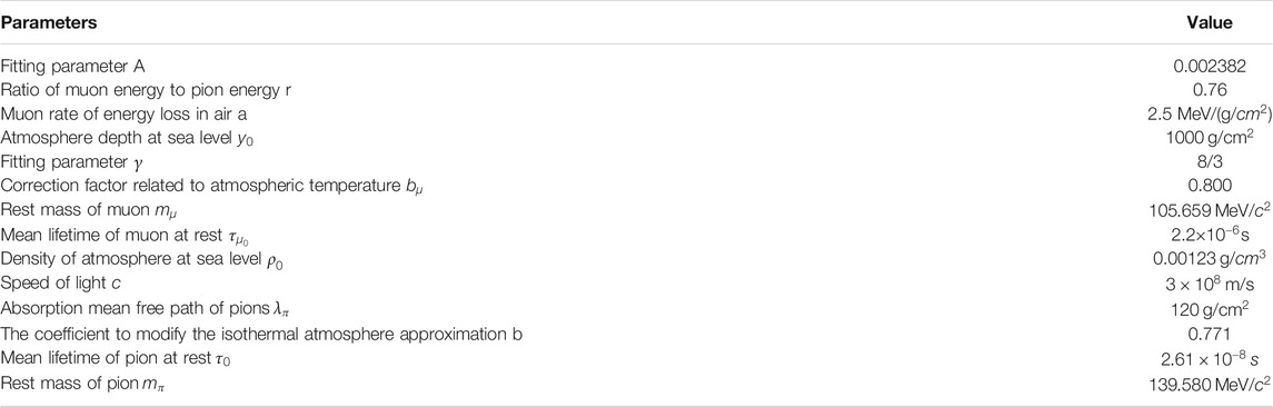
TABLE 2. Parameters in the Smith and Duller/Chatzidakis model (Chatzidakis et al., 2015).

Chatzidakis et al. compared their best fit model with Reyna model and experimental data from different experiments. The comparison results show that Smith and Duller/Chatzidakis model has slightly better accuracy than Reyna model in most cases.

Monte Carlo Simulation Model

Monte Carlo simulation models are generally based on theoretical models of physical processes, including the interaction between primary cosmic rays and the atmosphere, generation of muons by secondary cosmic ray decay, interaction between muons and the matter through which they transport, and decay of muons. The entire process is simulated, ranging from the generation of muons by primary cosmic ray incident into the atmosphere to their final arrival at sea level. In the simulation, some factors that will influence the flux and energy spectrum of muons are considered according to the requirement of accuracy, such as atmospheric curvature, solar modulation, geomagnetic cut-off rigidity, and ground conditions. Two types of Monte Carlo programs are used to simulate sea-level muons. One group contains models designed for general purposes, such as FLUKA, GEANT4, and PHITS, which can simulate the transport of various particles and their interaction with matter. The other group is designated for special purposes; these models specialize in the simulation of atmospheric showers or even focus on the generation and transport of cosmic ray muons and include CORSIKA, MUSIC, and CRY.

Among the Monte Carlo programs that can simulate sea-level cosmic ray muons, CRY is the most commonly used method in application. For example, CRY was used as a muon generator for the GEANT4 simulation of muon tomography for high-density materials (Thomay et al., 2016); it was also used as a cosmic ray muon background generator to simulate the response of an antineutrino reactor detector to background events (Ashenfelter et al., 2016). Because all of these Monte Carlo programs when simulating sea-level muons have basically identical principles, this section only introduces the most commonly used Monte Carlo model, CRY, as an example.

CRY is a software library that is, specifically used to generate information about air showers based on the simulation results of MCNPX 2.5.0. Secondary particles from a cosmic ray shower in the range of 1 MeV–100 TeV at three altitudes (0, 2100, and 11300 m) can be generated from the precomputed data table. The primary cosmic ray in the model is generated according to the empirical formula summarized by Papini et al. Solar modulation, latitude-dependent geomagnetic cut-off and altitude are also taken into account. The atmosphere was modelled according to the 1976 US atmosphere model, but the atmosphere model is flat and ignores the influence of atmospheric curvature on the attenuation of cosmic rays before reaching sea level (Hagmann et al., 2007).

Generally, both parametric analytical models and Monte Carlo models are based on the physical process of pion and kaon decay and the attenuation of muons in the process of penetrating the atmosphere. The consideration of atmospheric curvature serves as an option to improve the model’s accuracy. Comparing these two approaches, the parametric analytical model takes less time to generate sea-level muon distributions but has fewer variable parameters, thereby ignoring some factors that affect the sea-level muon flux. The Monte Carlo model simulates the entire physical process of muon production, which takes a very long time; however, it can flexibly modify the physical model and various factors.

Comparison With Experimental Data

According to the introduction in Muon Flux Model at Sea Level , the commonly used models of sea-level muon flux mainly describe the relationship between muon differential flux and muon energy, zenith angle. Therefore, in this section, the energy spectrum of the muon differential flux obtained by different models of sea-level muon flux is compared with the experimental data in specific zenith angle directions.

The models selected in this section include all aforementioned parametric analytical models and the Monte Carlo simulation model CRY. According to the features of the sea-level muon flux distribution and considering the available experimental data, two groups of experimental data in the direction of θ = 0° with the highest flux intensity and a large zenith angle of θ = 75° are selected for comparison with the above models.

Figures 2A,B show the comparison between the predicted values obtained by different models and the experimental data, where the data obtained by different experimental measurements in the same direction are represented by red dots, and differential fluxes obtained by parametric analytical models are represented by smooth solid lines of different colours. The dotted line in Figure 2 represents the result of CRY obtained by sampling ${10}^8$ primary cosmic ray protons at a latitude of 40°. The muon flux in the direction of θ = 0° is calculated by muons in the range of θ < 7°, while the muon flux in the direction of θ = 75° is calculated by muons in the range of 70°<θ < 80°. Figure 2 shows that in the direction of θ = 0°, the Gaisser model seriously overestimates the differential flux of muon below 10 GeV, but the other three parametric analytical models are consistent with the experimental data. In the large zenith angle direction of θ = 75°, the differential flux of muon is obviously overestimated by the Gaisser model below 100 GeV, while the muon energy spectrum obtained by CRY sampling has the same shape as the experimental data but is generally lower by approximately 80%. The overestimation of the muon flux in the low-energy region by the Gaisser formula is related to the fact that Eq. 2 ignores the decay and energy loss of muons in the transport process; the overall lower value produced by CRY sampling in the direction of the large zenith angle results from the flat atmosphere model, which overestimates the atmospheric thickness crossed by muons at a large zenith angle and underestimates the muon flux.

FIGURE 2

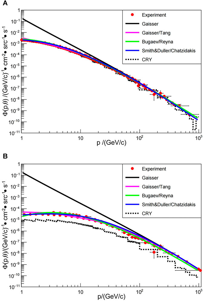
FIGURE 2. Comparison of the parametric analytical models and CRY to experimental data. (A): θ = 0° experimental data correspond to measurements from Refs (Achard et al., 2004; Tsuji et al., 1998; Haino et al., 2004; Nandi and Sinha, 1972); (B): θ = 75° experimental data correspond to measurements from Refs (Jokisch et al., 1979; Tsuji et al., 1998; Kellogg et al., 1978).

To further quantitatively compare the accuracy of the models in Figure 2, the goodness-of-fit of the models to the experimental data is evaluated by Pearson chi-square test. The formula of Pearson chi square test is as follows:

${\chi }^2={\displaystyle \sum }_{i=1}^n\frac{{({\phi }_i-f\left(E_i\right))}^2}{f\left(E_i\right)}(10)$

${\phi }_i$ in Eq. 10 represents the $i$th differential muon flux data measured by experiments in this direction, $E_i$ is the corresponding muon energy of the $i$th experimental data point, and $f\left(E_i\right)$ is the theoretical value of the muon flux obtained by the models at energy $E_i$. A smaller ${\chi }^2$ corresponds to a better model.

Figure 3 shows the comparison results of the ${\chi }^2$ of the models. The experimental data correspond to measurements from Refs (Jokisch et al., 1979; Achard et al., 2004; Tsuji et al., 1998; Haino et al., 2004; Kellogg et al., 1978) within the muon momentum range below 1,000 GeV/c. There are 119 data points in the 0° direction and 58 data points in the 75° direction. Figure 3 shows that${\chi }^2$ of the Gaisser model in the direction of θ = 0° is considerably higher than that of the other models. In the direction of θ = 75°, ${\chi }^2$ of Gaisser is still the largest among all models, and ${\chi }^2$ of CRY is also significantly higher than that of the other three parametric analytical models. The fitting of ${\chi }^2$ under the Gaisser/Tang, Bugaev/Reyna, and Smith and Duller/Chatzidakis models becomes closer in the direction of θ = 75° than that in the direction of θ = 0°.

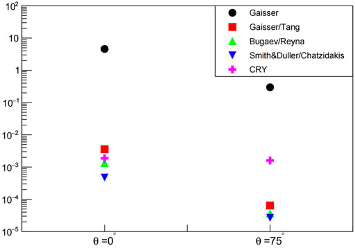
FIGURE 3

FIGURE 3. ${\chi }^2$ of different sea-level muon modes in different directions.

From the comparison results, we observe a large deviation in the original Gaisser model in describing the distribution of muon fluxes, and CRY underestimates the distribution of muon fluxes at large zenith angles. The remaining three models are relatively accurate when describing the distribution of muon fluxes. Since the energy and zenith angle range of interest varies in different applications of muons, the selection of sea level muon models should be determined according to the concerned region. For example, underground experiments mainly focus on cosmic ray muons with TeV energy at sea level, so the Gaisser model can be used in this situation. Muon imaging mainly focuses on several to hundreds of GeV medium-energy muons, where the Gaisser model should be avoided. As for muon imaging of volcanos which utilizes near-horizontal muons, CRY is not recommended.

Conclusion

In this paper, we summarize several commonly used models to describe sea-level cosmic ray muon flux distribution from two aspects: parametric analytical models and Monte Carlo models. The comparison of these models show that the commonly-used Gaisser model and Monte Carlo model CRY produce a large error when describing sea-level muon fluxes. Gaisser model overestimates muon flux in the low-energy region while CRY underestimates it at large zenith angles. The muon flux models given by Gaisser/Tang, Bugaev/Reyna, and Smith and Duller/Chatzidakis are consistent with the experimental results. In practical applications, we must consider the desired muon energy and angle range to select the appropriate sea-level muon description model.

Data Availability Statement

The original contributions presented in the study are included in the article/Supplementary Material, further inquiries can be directed to the corresponding authors.

Author Contributions

NS conducted the research and wrote the paper. YL designed the research. LW supervised the study and cowrote the paper. BW proposed the method to compare the models. JC provided guidance throughout the research.

Funding

This work is supported by the Key Lab of Particle and Radiation Imaging, Ministry of Education (20180102) and the Central University Basic Scientific Research Business Expenses Special Funds under the project name of Research on Applied Physics under Low Radiation Background (Grant No. 2018NTST07).

Conflict of Interest

The authors declare that the research was conducted in the absence of any commercial or financial relationships that could be construed as a potential conflict of interest.

Publisher’s Note

All claims expressed in this article are solely those of the authors and do not necessarily represent those of their affiliated organizations, or those of the publisher, the editors and the reviewers. Any product that may be evaluated in this article, or claim that may be made by its manufacturer, is not guaranteed or endorsed by the publisher.

References

Achard, P., Adriani, O., Aguilar-Benitez, M., van den Akker, M., Alcaraz, J., Alemanni, G., et al. (2004). Measurement of the Atmospheric Muon Spectrum from 20 to 3000 GeV. Phys. Lett. B. 598 (1-2), 15–32. doi:10.1016/j.physletb.2004.08.003

CrossRef Full Text | Google Scholar

Ashenfelter, J., Balantekin, B., and Band, H. R. (2016). The PROSPECT Physics Program. J. Phys. G: Nucl. Part. Phys. 43 (11), 113001.

Google Scholar

Bugaev, E. V., Misaki, A., Naumov, V. A., Sinegovskaya, T. S., Sinegovsky, S. I., and Takahashi, N. (1998). Atmospheric Muon Flux at Sea Level, Underground, and Underwater. Phys. Rev. D 58 (5), 054001. doi:10.1103/PhysRevD.58.054001

CrossRef Full Text | Google Scholar

Chatzidakis, S., Chrysikopoulou, S., and Tsoukalas, L. H. (2015). Developing a Cosmic ray Muon Sampling Capability for Muon. Nucl. Instrum. Meth. A. 804, 33–42. doi:10.1016/j.nima.2015.09.033

CrossRef Full Text | Google Scholar

Fujii, H., Hara, K., Hayashi, K., Kakuno, H., Kodama, H., Nagamine, K., et al. (2020). Investigation of the Unit-1 Nuclear Reactor of Fukushima Daiichi by Cosmic Muon Radiography. Prog. Theor. Exp. Phys. 2020 (4), 043C02. doi:10.1093/ptep/ptaa027

CrossRef Full Text | Google Scholar

Gaisser, T. K. (1990). Cosmic Rays and Particle Physics. New York: Cambridge University Press.

Google Scholar

Guo, Z.-y., Bathe-Peters, L., Chen, S.-m., Chouaki, M., Dou, W., Guo, L., et al. (2021). Muon Flux Measurement at China Jinping Underground Laboratory *. Chin. Phys. C 45 (2), 025001. doi:10.1088/1674-1137/abccae

CrossRef Full Text | Google Scholar

Hagmann, C., Lange, D., and Wright, D. (2007). “Cosmic-ray Shower Generator (CRY) for Monte Carlo Transport Codes” in 2007 IEEE Nuclear Science Symposium Conference Record, 2, 1143–1146. doi:10.1109/NSSMIC.2007.4437209

CrossRef Full Text | Google Scholar

Haino, S., Sanuki, T., Abe, K., Anraku, K., Asaoka, Y., Fuke, H., et al. (2004). Measurements of Primary and Atmospheric Cosmic-ray Spectra with the BESS-TeV Spectrometer. Phys. Lett. B 594 (1-2), 35–46. doi:10.1016/j.physletb.2004.05.019

CrossRef Full Text | Google Scholar

Jokisch, H., Carstensen, K., Dau, W. D., Meyer, H. J., and Allkofer, O. C. (1979). Cosmic-ray Muon Spectrum up to 1 TeV at 75° Zenith Angle. Phys. Rev. D 19 (5), 1368–1372. doi:10.1103/PhysRevD.19.1368

CrossRef Full Text | Google Scholar

Kellogg, R. G., Kasha, H., and Larsen, R. C. (1978). Momentum Spectra, Charge Ratio, and Zenith-Angle Dependence of Cosmic-ray Muons. Phys. Rev. D 17 (1), 98–113. doi:10.1103/PhysRevD.17.98

CrossRef Full Text | Google Scholar

Morishima, K., Kuno, M., Nishio, A., Kitagawa, N., Manabe, Y., Moto, M., et al. (2017). Discovery of a Big Void in Khufu's Pyramid by Observation of Cosmic-ray Muons. Nature 552 (7685), 386–390. doi:10.1038/nature24647

PubMed Abstract | CrossRef Full Text | Google Scholar

Nandi, B. C., and Sinha, M. S. (1972). The Momentum Spectrum of Muons at Sea Level in the Range 5-1200 GeV/c. J. Phys. A: Gen. Phys. 5 (9), 1384–1394. doi:10.1088/0305-4470/5/9/011

CrossRef Full Text | Google Scholar

Reyna, D. (2006). A Simple Parameterization of the Cosmic-Ray Muon Momentum Spectra at the Surface as a Function of Zenith Angle. arXiv [Preprint] Available at: https://arxiv.org/abs/hep-ph/0604145v2 (Accessed July 29, 2021).

Google Scholar

Smith, J. A., and Duller, N. M. (1959). Effects of Pi Meson Decay-Absorption Phenomena on the High-Energy Mu Meson Zenithal Variation Near Sea Level. J. Geophys. Res. 64 (12), 2297–2305. doi:10.1029/JZ064i012p02297

CrossRef Full Text | Google Scholar

Tang, A., Horton-Smith, G., Kudryavtsev, V. A., and Tonazzo, A. (2006). Muon Simulations for Super-kamiokande, KamLAND, and CHOOZ. Phys. Rev. D 74 (5), 53007. doi:10.1103/PhysRevD.74.053007

CrossRef Full Text | Google Scholar

Thomay, C., Velthuis, J., Poffley, T., Baesso, P., Cussans, D., and Frazão, L. (2016). Passive 3D Imaging of Nuclear Waste Containers with Muon Scattering Tomography. J. Inst. 11 (3), P03008. doi:10.1088/1748-0221/11/03/P03008

CrossRef Full Text | Google Scholar

Tsuji, S., Katayama, T., and Okei, K. (1998). Measurements of Muons at Sea Level. J. Phys. G: Nucl. Part. Phys 24 (9), 1805–1822. doi:10.1088/0954-3899/24/9/013

CrossRef Full Text | Google Scholar

Turko, J., Pillalamarri, I., and Jagam, P. (2020). GEANT4 Simulations of Cosmic Muon Background in CEMRC BEGe Lung Detectors and Detection Sensitivity Optimization of Trans-uranic Radionuclides. J. Radiat. Res. Appl. Sci. 13 (1), 111–120. doi:10.1080/16878507.2019.1711341

CrossRef Full Text | Google Scholar