 Yujun Su1
 Mingyao Zou
94% of researchers rate our articles as excellent or good
Learn more about the work of our research integrity team to safeguard the quality of each article we publish.
Find out more
ORIGINAL RESEARCH article
Front. Energy Res., 14 October 2021
Sec. Electrochemical Energy Storage
Volume 9 - 2021 | https://doi.org/10.3389/fenrg.2021.738556
This article is part of the Research TopicArtificial Intelligence Applications in Low Carbon Renewable Energy and Energy Storage SystemsView all 8 articles
As to the nonlinear and time-varying problems of the energy consumption model, this paper proposes an adaptive hybrid modeling method. Firstly, the recursive least squares algorithm with adaptive forgetting factor based on fuzzy algorithm and recursive least squares algorithm is used to identify the simplified mechanism energy consumption model, which solves the data saturation phenomenon and the weights of the “old and new” data during the online identification process and guarantees the adaptability of the mechanism model. Secondly, because there is a deviation between the identified model and the simplified mechanism energy consumption model, the deviation compensation model of mechanism model is established through kernel partial least squares algorithm and the model updating strategy with sliding window, which is used to update the deviation compensation model, and then the adaptive hybrid model is established by combining with the mechanism model identified online and updated deviation compensation model. Finally, the effectiveness, generalization and adaptability of the model are verified by the actual operating data of a single working condition and variable working conditions. And comparing with the mechanism model and the data model, The comparison results show that the adaptive hybrid model has higher calculation accuracy with adaptation.
As to the nonlinear and time-varying problems of the energy consumption model, in order to obtain the optimal operating parameters for the maximum energy efficiency, it is necessary to establish an accurate energy consumption model. However, the mechanism model of energy consumption has non-linearity and time variation under different working conditions and outdoor temperature, and even could not completely reflect characteristic of the energy consumption model(Li and Zaheeruddin, 2019; Foliaco et al., 2020; Tudoroiu et al., 2020). Thus, an effective method is supposed to research to obtain precise energy consumption model.
At present, the mechanism model based on the physical conception of equipment or physical characteristics of equipment, such as based on law of thermodynamics, the model structure was established by means of effective volume method, grid-search method, integral order and step size(Mazimbo et al., 2019). And in order to obtain the simplified mechanism model, we need use identification method to get the parameters of the simplified mechanism model. In general, the recursive least squares algorithm with fixed forgetting factor (Shi et al., 2016; Xia et al., 2018) is widely used to identify the model’s parameters of the object, due to its simple principle, small computational complexity and the function of online identification. Nevertheless, the recursive least squares algorithm with fixed forgetting factor has poor tracking ability when the working conditions appears in changing. (Pang and Cui, 2017) Therefore, it cannot well solve the time-varying problem of the parameters of the mechanism model.
Differ from the mechanism modeling method, the data modeling method(Ji et al., 2016; Malbasa et al., 2017; Wu and Wang, 2018; Liu, 2019; Moreira et al., 2019; Wu et al., 2019) uses the data to construct the model of the controlled object. Through the neural network method(Zhang, 2018), an efficient model for high frequency electronics and microwave circuits was established. And on the premise of having enough historical operation data as samples, through the analysis of support vector machine, data mining technology (Patnaik et al., 2010) was used to establish the dynamic Bayesian network model, and the energy consumption model was created based on the machine learning method (Park et al., 2019). However, the generalization ability of the data model is related to the coverage of the samples, but it is difficult to obtain enough global samples in actual field. If the samples contain local working conditions, the generalization ability of the data model is limited and cannot solve the nonlinearity problem of the model parameters under global situation.
In order to improve the calculation accuracy of model and reduce the amount of modeling calculation, the hybrid modeling has been deeply studied and widely used in many fields(Chou et al., 2013; Yao et al., 2016; Guo and Wang, 2017; Hamilton et al., 2017). A method combining mechanism analysis with data driven compensation method was proposed, and a hybrid model of the electrostatic precipitators (ESP)(Guo et al., 2018) and one data driven hybrid model (Li et al., 2018) for short-term traffic flow prediction were established. Nevertheless, the data driven requires a large amount of global data to train to obtain accurate deviation compensation model. It require high costs. Applying this idea to the Hybird Energy Consumption Model, using physical and empirical modeling methods (Jin et al., 2011); (Xu, 2017) But all of the above are based on the study of single operating conditions. There is a large error between actual value and calculation value of the model under variable operating conditions, and it does not have good adaptability.
To solve the above mentioned problems, the main contributions of the paper include:
1) To solve the data saturation phenomenon and the weights of the “old and new” data during the online identification process, a recursive least squares algorithm with adaptive forgetting factor, which integrates fuzzy algorithm with recursive least squares (RLS) algorithm is proposed, It gets to identify the parameters of the mechanism model and guarantees the adaptability of the mechanism model.
2) Aiming at the discrepancy between identified model and the simplified mechanism energy consumption model, the deviation compensation model of mechanism model is established through kernel partial least squares algorithm and the model updating strategy with sliding window, which is used to update the deviation compensation model.
This paper is organized as follows. We introduce the structure of the adaptive hybrid model, and establish the mechanism model, and then the model’s parameters are identified online by adaptive forgetting factor recursive least squares algorithm based on fuzzy algorithm and recursive least squares algorithm in Section 2. In section 3, under getting the mechanism model online in section 2, we combine kernel partial least squares algorithm and model updating strategy with sliding window to establish the adaptive hybrid model. The actual running data is obtained to verify the effectiveness, generalization and adaptability of the adaptive hybrid model in Section 4. It is the concluding part of this paper in Section 5.
In this section, the adaptive hybrid energy consumption model is proposed, and the simplified mechanism model is obtained online with adaptive forgetting factor through combining with fuzzy algorithm and recursive least squares algorithm.
The structure of adaptive hybrid model is shown in Figure 1,with the non-linearity and time variation of the mechanism model of the energy consumption model, RLS algorithm with adaptive forgetting factor, which integrates fuzzy algorithm and RLS algorithm, puts forward to quickly and precisely identify the parameters of the mechanism online, and it can guarantee the effectiveness of the mechanism model when the working conditions changes. Therefore, the k-th output ym(k) of the mechanism model can be obtained through the above online identification method when the mechanism model input values, α1, α2, …, αn, are detected in real time. However, it exists the deviation with the actual characteristics of the energy consumption model. A data-driven way, the kernel partial least squares (KPLS) algorithm, is used to form the deviation compensation model. Meanwhile, in order to improve the adaptability of the deviation compensation model, the deviation compensation model is updated by sliding window. So the k-th real-time output yd(k) of the deviation compensation model can be gotten when the mechanism model inputs α1, α2, …, αn, the other detected parameters β1, β2, …, βn and last step

FIGURE 1. The structure of adaptive hybrid model.
Among Them:
where
Therefore, the output of the adaptive hybrid model is:
An adaptive forgetting factor RLS algorithm is proposed based on fuzzy algorithm and RLS algorithm to identify the mechanism model online, and the structure of this algorithm is shown in Figure 2. We continuously detects the real-time input value α1, α2, …, αn of model and the energy consumption Y in the process of online operation, and then we obtain the time series average W of the residual and its change rate ΔW between the deviation of the system dynamic characteristic value and the identified model value, taking them as the inputs of the fuzzy algorithm. In this way, we can acquire the adjusted forgetting factor’s value μ in real time, and bring it into Eq. 4 to get the parameters
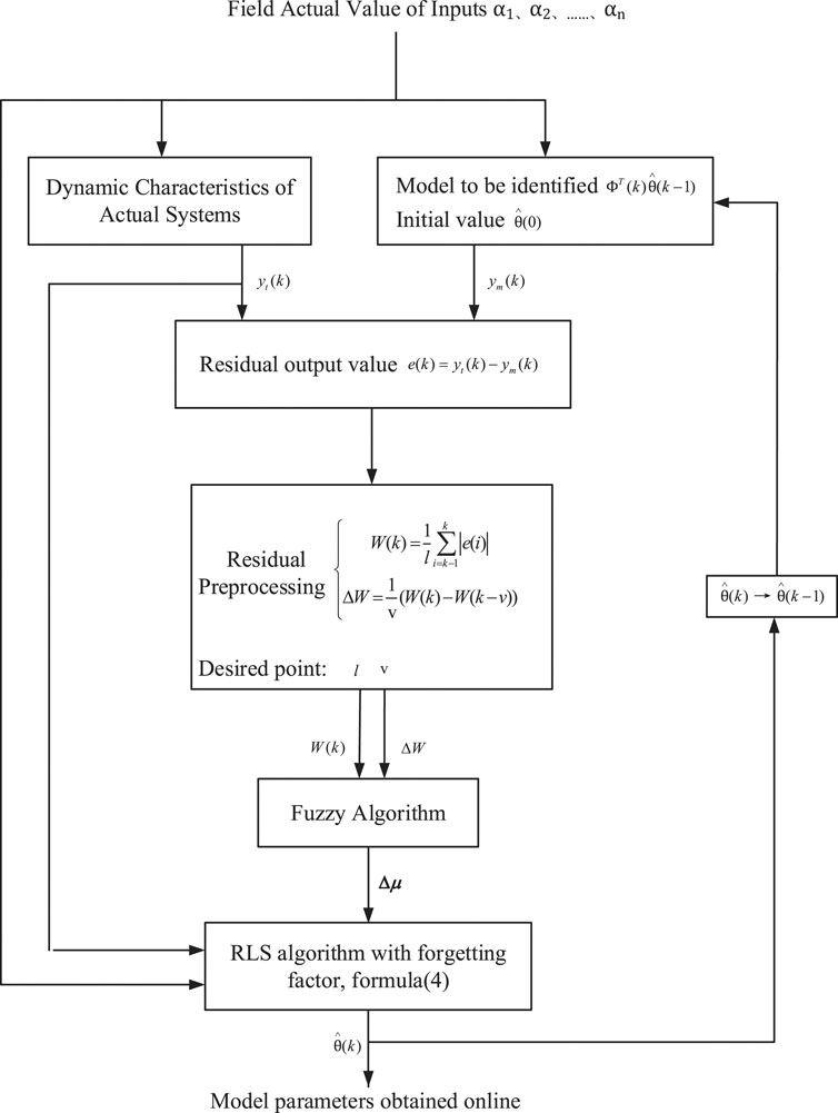
FIGURE 2. Model identification of adaptive forgetting factor RLS algorithm.
RLS algorithm is widely used for online identification of model parameters because of its simple principle, small computational complexity, low memory consumption, and can be used for online real-time estimation of parameters. The RLS algorithm is suitable for the constant unknown parameter system. For the time-varying problem of the parameters, the RLS has its limitations. When the system parameters change, the RLS algorithm will not be able to track this change, which will reduce the accuracy of the real-time parameters estimation or even fail. In order to solve the above phenomenon, each new data is given a weight to improve the algorithm to form a forgetting factor RLS algorithm. The iterative calculation formula through using forgetting factor recursive least squares algorithm7 and combining with the mechanism model is:
where ΦT(k) is a covariance matrix; K(k) is a gain matrix;
In the process of the online identification of the time-varying system, if the residual difference between the dynamic deviation value and the identification model value of the system at the time of the k-time is:
where
The magnitude of the absolute value of the residual reflects the difference between the system dynamic deviation value and the identification model value. In the process of parameter online identification, the bigger the absolute residual value is, at this time, the smaller the strain of forgetting factor is, so that the identification result of the RLS algorithm quickly converges to the vicinity of the actual model parameters. When the absolute residual value becomes smaller, it is hoped that the forgetting factor will become larger to suppress noise disturbance to the influence of the accuracy of parameter identification.
If the forgetting factor is corrected only by the absolute value of a single residual, there is a large contingency and error, and the forgetting factor is sensitive to noise interference in the process of correction. Therefore, the mean value of a time series of absolute errors is used as the evaluation function W of the degree of approximation between the identified parameters and the actual parameters. At the time of k, the calculation formula is as follows:
where l is the time series length of the residual.
From the above analysis, the correction value of forgetting factor is negatively correlated with the evaluation function. In order to accurately describe the relationship between them, this paper corrects the forgetting factor online and real-time through the fuzzy algorithm, and the evaluation function is used as an input of fuzzy algorithm. Meanwhile, the change rate of the evaluation function ΔW over a period of time can more accurately reflect the trend of the identification error. Thus, ΔW can be used as another input of the fuzzy algorithm. The calculation of the k time is as follows:
where v is the time constant discrete value of the change rate of the evaluation function.
In this paper, the fuzzy algorithm is used to realize the online correction of the forgetting factor. The mean residuals over a period of time W and the residual change rate ΔW are used as the inputs of the fuzzy algorithm. And then the modified value Δμ is the output of the fuzzy algorithm. The adaptive adjustment of forgetting factor is realized, as shown in Figure 3.
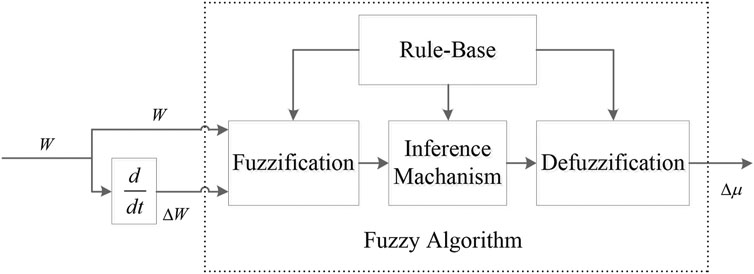
FIGURE 3. Adaptive adjustment of forgetting factor based on Fuzzy Algorithm.
In the adaptive correction process of the forgetting factor of the fuzzy algorithm, the value of W, ΔW and Δμ are fuzzed, and the fuzzy domains of W is [−10,10], and the fuzzy domains of ΔW is [−2,2]. In the recursive least squares algorithm, the forgetting factor is usually 0.9 ≤ μ ≤ 1, so the fuzzy domain of Δμ is [−0.1, 0.1]. In addition, the input of the fuzzy control rules and the linguistic variables of the premise constitute the fuzzy input space, and the linguistic variables of the conclusion form the fuzzy output space. Therefore, the W, ΔW and modified value Δμ are segmented by a fuzzy method, and their fuzzy sets are obtained as follows (Jiang et al., 2020):
The fuzzy set of W is {NB,NS,ZO,PS,PB}; The fuzzy set of ΔW is {NB,NS,ZO,PS,PB}; The fuzzy set of Δμ is {NB,NM,NS,ZO,PS,PM,PB}.
According to the tentative method, selecting the Gaussian function as the membership function of the W, ΔW, and modified value Δμ, and their membership functions are shown in Figures 4A,B,C
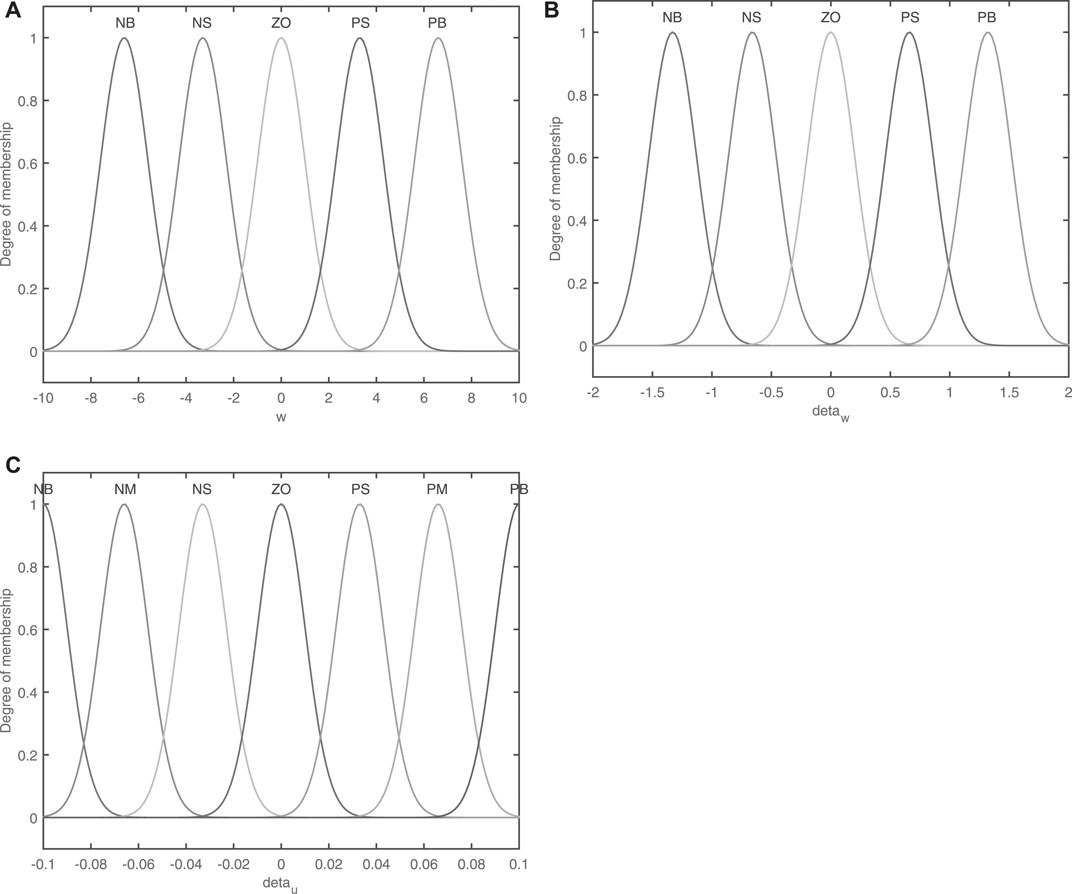
FIGURE 4. Membership function.
In the fuzzy algorithm, the fuzzy control rule is an important part of it and can be represented by the fuzzy rule table. The fuzzy rule base is a linguistic expression form based on expert knowledge or long-term accumulated experience and human intuitive reasoning. When both W and ΔW are poslarge, the deviation between the predicted value and the actual value is large, at this time, Δμ is selected to be neglarge. When W is poslarge and ΔW is neglarge, the deviation between the predicted value and the actual value is large, but gradually decreases, Δμ is negsmall. When both W and ΔW are neglarge, the identification parameter value is very close to the actual parameter value, Δμ is poslarge. When W is neglarge, ΔW is negsmall, the expected correction value Δμ is possmall. Based on the above knowledge, the fuzzy control rules of Table 1 can be established.
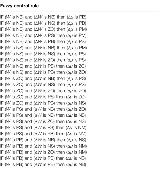
TABLE 1. Fuzzy control rule table.
From the fuzzy rules established in Table 1, the fuzzy rule table of 5 × 5 in Table 2 can be obtained.

TABLE 2. Fuzzy control rule table.
According to the fuzzy rule table formulated in Table 2, the forgetting factor’s correction value Δμ is calculated by Mamdani fuzzy inference and Centroid defuzzification. According to the forgetting factor’s correction value Δμ obtained in real time, the forgetting factor is corrected to:
where μ0 is the initial value of the forgetting factor.
According to the estimated parameter convergence theorem(Li et al., 2018), when the input is persistently exciting of order N, it can make the
In this section, the deviation consumption model of the simplified mechanism model is got by kernel partial least squares algorithm, and using model updating strategy with sliding window to update the deviation compensation model. And combining with the online identified model which has been obtained with the adaptive forgetting factor RLS algorithm in section 2, the adaptive hybrid energy consumption model is established.
Through the section 2, the real-time output ym(k) of the simplified mechanism model can be obtained. However, in the process of mechanism modeling, the mechanism model is deviated from the actual characteristics. In addition, in the case of production process or external disturbances, it will cause errors between the actual model and the simplified mechanism model.
Therefore, the kernel partial least squares algorithm is used to establish the deviation compensation model of the simplified mechanism model. it makes the calculated deviation yd(k) be the output of the deviation compensation model.
If the variable X ∈ Rn×p, Y ∈ Rn×q, and p is the number of independent variable, q is the number of dependent variable, n is the number of observed samples, the nonlinear mapping from the original input space
In the mapping space, the weight vector ω1 and c1 of X are determined according to the mapped sample matrices Φ and Y. Under the constraint of
The lagrangian function is established for the above.
η1, η2 are the Lagrangian multiplier, and the partial derivatives of L(ω1, Φ, Y, c1) to ω1, c1, η1, η2 are respectively divided into 0.
Therefore
where “0” is the original data, ω1 is the eigenvector λ1 corresponding to the largest eigenvalue of
Then the kernel matrix is
where Kα,β is the selected kernel function.
In this paper, the kernel matrix is used Gaussian kernel function to gotten. its expression is:
where σ is the width of the Gaussian kernel function, x is the data sample, α, β is the the data sequence.
After obtaining the first kernel principal component t1, and the centralized kernel residual matrix
where
The residual matrix Fi of the centralized dependent variable data matrix is
So the remaining kernel principal components are obtained:
Similarly, the kernel principal component ui can be obtained according to the independent variable data matrix E0. And the matrix ti, ui are composed of T, U.
Therefore, the output of the KPLS algorithm can be expressed as:
Through the above mentioned, the deviation compensation model of mechanism model is established by kernel partial least squares algorithm.
However, with the changes in working conditions and mechanism model parameters, the nonlinear relationship between the deviation of mechanism model and its inputs are constantly changing. So this paper uses the model updating strategy with sliding window to update the kernel matrix of the deviation compensation model in real time, and improve the prediction accuracy of the model. The sliding window updating strategy is to set a fixed-length sample as a training sample, and to make the window slide forward with the acquisition of the new sample, thereby implementing the update of the model. The purpose of the deviation compensation model updating is to update the elements in the kernel matrix to adapt the adaptability of the model when operating conditions change. It is only necessary to change the position of some elements and calculate a small number of new elements during the updating process without having to perform a lot of double counting.
The updating process of the deviation compensation model is shown in Figure 5. Consuming the window length to be g,then the kernel is Kg×g, and the sliding length is q. So when the sliding window slides forward, the new input and output data are got to form the updated samples. The updated input samples are recorded as X* and the updated output samples are recorded as Y*. Firstly, the kernel matrix is renewed by the updated samples X* and Y* through the kernel function. The kernel matrix updating process is as follows: to begin with, deleting the matrix elements corresponding to the discarded q samples, then changing the position of the reserved elements, and finally calculating the corresponding elements of the q new samples and adding them to the kernel matrix to complete the updating of the model.
1) Deleting old samples
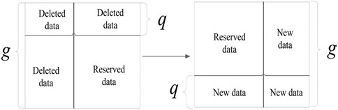
FIGURE 5. The updating process of the deviation compensation model.
For the variable x ∈ Rg, the expression of the kernel matrix
For the current running state of the modeled object, the first q group samples are old sample points with no value, and the elements containing x1 ∼ xq in the kernel matrix should be deleted. After deleting the corresponding elements, the kernel matrix is recorded as
2) Adding new samples
After deleting the old samples, in order to maintain the order of the kernel matrix, it is necessary to add the same number of new samples. Since the updating model adopts the timing update strategy, the newly added matrix elements need to consider the sample timing, and the kernel matrix after adding the new elements is recorded as
Secondly, the new score vector T* and U* can be gained by Eqs 9–18 according to the updated samples X* and Y*.
Finally, the output yd(k) of the adaptive deviation compensation model through the KPLS algorithm and the model updating strategy with sliding window is:
where yd(k) is the output of the adaptive deviation compensation model.
Through the content introduced above, the recursive least squares algorithm with adaptive forgetting factor, kernel partial least squares algorithm and the model updating strategy with sliding window are used to established the adaptive hybrid model. And the modeling steps are as follows:
1) Obtaining the running real-time/ historical data, and excluding outliers.
2) Establishing the mechanism model, and identifying the model parameters
3) Calculating the output ym(k) of the identified mechanism model at k-time, and calculating the deviation between the actual model and identified model at this time;
4) Sliding the sliding window to update the data to update the kernel matrix;
5) Calculating the output yh(k) of the deviation compensation model at k time by using real-time and historical data;
6) Superimposing the output of the deviation compensation model and the mechanism model to obtain the output yh(k) = ym(k) + yd(k) of the adaptive hybrid model.
In this section, we use the field operation data of a signal centrifugal chiller to verify the accuracy, generalization and adaptability of the adaptive hybrid model proposed in this paper.
The simplified energy consumption model (Bozorgian, 2020) can be expressed as follows.
where ym is the energy consumption; Qnom is the rated refrigeration capacity, it is 2813 kW in this paper; COPnom is the rated refrigeration efficiency, it is 6.86 in this paper; PLRadj is load rate; TCHWS is the supply water temperature; TCWS is the supply water temperature of cooling water; ai(k) is the model parameter to be identified, i = 0, 1, 2, 3, 4, 5.
According to the analysis in the previous section, combined with the chiller model, from formula , we can get ΦT(k) and X, Y are as follow:
In this paper, the field operation data of a signal chiller in a data center are taken as samples, and the operation status of the chiller at a 26–27°C wet bulb temperature is taken as working condition 1, the operation status of the chiller at a 25–26°C wet bulb temperature is taken as working condition 2, and the operation status of the chiller at a 24–25°C wet bulb temperature is taken as working condition 3.Under this premise, the energy consumption of the chiller model is different at different circumstance temperature ranges, and the parameters of the corresponding model change, which means that the model is time-varying. In addition, the time series length of residual is set to l = 7, and the time constant discrete value of change rate of the evaluation function is v = 14. Finally, the adaptive hybrid dynamic energy consumption model is verified by the sample data under single working condition (working condition 2), to make the working condition data non-repetitive, working conditions 1 and 3 are chosen to study the calculation accuracy comparison of different models under variable conditions. The root mean square error (RMSE) and mean absolute percentage error (MAPE) are used to evaluate the accuracy of the model.
Under working condition 2, there are 1087 sets of actual data, and 965 sets of global data are selected as training data, and 122 sets of global data are used as test data. Respectively, through mechanism model, data model (Kernel Partial Least Squares model) and adaptive hybrid model to compare the model accuracy. The training and test effects of mechanism model is shown as Figure 6, the effects of KPLS model is shown as Figure 7, and the effects of adaptive hybrid model is shown as Figure 8.calculation accuracy of different models under signal working condition (working condition 2) is shown in Table 3.
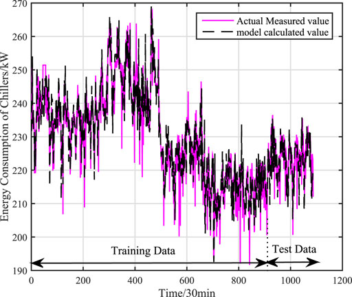
FIGURE 6. Training and test results of mechanism model under single working condition (working condition 2).
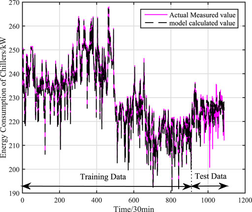
FIGURE 7. Training and test results of KPLS model under single working condition (working condition 2).
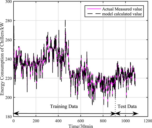
FIGURE 8. Training and test results of adaptive hybrid model under single working condition (working condition 2).
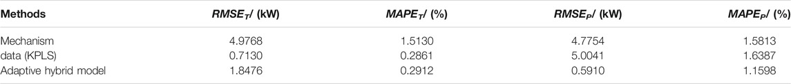
TABLE 3. Calculation accuracy of different models under signal working condition (working condition 2).
It can be concluded from Figures 6, 7, 8 that the adaptive hybrid model has higher fitting accuracy and better generalization ability, and can track the energy consumption change in time. From Table 3, we can see that the accuracy of the mechanism model is poor, because the mechanism model ignores some factors that affect the power consumption of water chillers, resulting in larger errors in the mechanism model. The data (KPLS) model has a higher Accuracy, but the prediction accuracy of the model is low, the model has over-fitting phenomenon and thus affects the prediction accuracy of the model. Comparing with the mechanism model and the data model, the root mean square error of the adaptive hybrid model is reduced by 87.6 and 88.2% respectively, and the average absolute percentage error is reduced by 89.9 and 90.2% respectively. The model has higher accuracy.
This paper further verifies the prediction accuracy, generalization and adaptability of the adaptive hybrid model under variable working conditions by using the actual data of centrifugal chiller under working conditions 1 and 3. There are 954 sets of actual data in working condition 1 and all of them are used as training data. There are 590 sets of actual data in working condition 3 and all of them are used as test data. The accuracy of mechanism model under variable working conditions is shown as Figure 9. The accuracy of data (KPLS) model under variable working conditions is shown as Figure 10. The faccuracy of adaptive hybrid model under variable working conditions is shown as Figure 11.the calculation accuracy of different models under multiple working conditions is shown in Table 4.
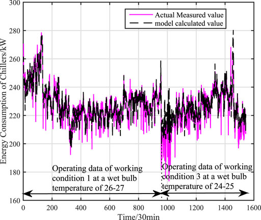
FIGURE 9. The accuracy of mechanism model under multiple working conditions (working condition 1 and working condition 3).
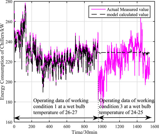
FIGURE 10. The accuracy of KPLS model under multiple working conditions (working condition 1 and working condition 3).
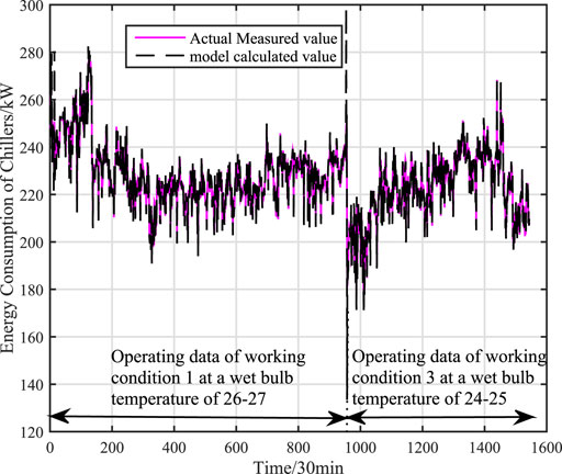
FIGURE 11. The accuracy of adaptive hybrid model under multiple working conditions (working condition 1 and working condition 3).

TABLE 4. Calculation accuracy of different models under multiple working condition (working condition 1 and working condition 3).
From the Figure 10, it can be concluded that the calculation accuracy of data (KPLS) model has a large deviation under variable working conditions, because the dynamic characteristics of chillers will change when the external temperature changes, while the training samples contain limited working data. When the data contain the number of new working conditions, data (KPLS) model will occur to lose effectiveness, which seriously affects the accuracy of the model. However, the adaptive hybrid model has better generalization and adaptability when the working condition changes from working condition 1 to working condition 3. The root mean square error is reduced by 61.8 and 77.2% respectively compared with the mechanism model and the data model, and the average absolute percentage error is reduced by 85.4 and 92.6% respectively compared with the mechanism model and the data model.
From the analysis of the above results, it can be seen that the adaptive hybrid model not only guarantees high fitting accuracy, but also has high generalization ability and adaptability. Compared with the mechanism model, the adaptive hybrid model accurately describes the dynamic characteristics of the centrifugal chiller, avoiding the negative impact of the lack of input variables on the accuracy of the model. Compared with the data model, the accuracy of the adaptive hybrid model is not affected by the coverage of training samples, and it also avoids the over-fitting phenomenon. In addition, the adaptive hybrid model also has high adaptability to variable working conditions.
In order to describe the dynamic characteristics of objects better and more accurately, an adaptive hybrid modeling method is proposed in this paper. To begin with, the mechanism model of the object is established by mechanism analysis, and to quickly and accurately identify the parameters of time-varying model online, a recursive least squares algorithm with adaptive forgetting factor is proposed in combination with fuzzy algorithm and recursive least squares algorithm, which ensures the validity of the parameters of the model. Secondly, the deviation compensation model of the object’s mechanism model is established by using the kernel partial least squares algorithm, and the model updating strategy with sliding window is used to modify the deviation compensation model, so as to construct the adaptive hybrid model of the object. Finally, the field running data of centrifugal chillers under signal and variable working conditions verifies that the adaptive hybrid model can not only quickly and accurately identify the model parameters online, but also has good validity, generalization and adaptability. At the same time, comparing with the mechanism and data model, the adaptive hybrid model also has higher accuracy.
The original contributions presented in the study are included in the article/Supplementary Material, further inquiries can be directed to the corresponding author.
All authors listed have made a substantial, direct, and intellectual contribution to the work and approved it for publication.
This work is supported by Shanghai “Science and Technology Innovation Action Plan High-tech Field Project”(19511103700).
The authors declare that the research was conducted in the absence of any commercial or financial relationships that could be construed as a potential conflict of interest.
All claims expressed in this article are solely those of the authors and do not necessarily represent those of their affiliated organizations, or those of the publisher, the editors, and the reviewers. Any product that may be evaluated in this article, or claim that may be made by its manufacturer, is not guaranteed or endorsed by the publisher.
The Supplementary Material for this article can be found online at: https://www.frontiersin.org/articles/10.3389/fenrg.2021.738556/full#supplementary-material.
Bozorgian, A. (2020). Analysis and Simulating Recuperator Impact on the Thermodynamic Performance of the Combined Water-Ammonia Cycle. Prog. Chem. Biochem. Res. 3 (2), 169–179. doi:10.33945/sami/pcbr.2020.2.10
Chou, J.-S., Tsai, C.-F., and Lu, Y.-H. (2013). Project Dispute Prediction by Hybrid Machine Learning Techniques. J. Civil Eng. Manag. 19 (4), 505–517. doi:10.3846/13923730.2013.768544
Foliaco, B., Bula, A., and Coombes, P. (2020). Improving the Gordon-Ng Model and Analyzing Thermodynamic Parameters to Evaluate Performance in a Water-Cooled Centrifugal Chiller. Energies 13 (9), 2135. doi:10.3390/en13092135
Guo, Y. H., and Wang, Q. (2017). “Research on Network Workload Resource Prediction Based on Hybrid Model,” in 2017 8th IEEE International Conference on Software Engineering and Service Science (ICSESS), Nov. 2017, Beijing, China, November 24–26, 2017 (IEEE), 24–26. doi:10.1109/icsess.2017.8343053
Guo, Y., Zheng, C., Xu, Z., Yang, Z., Weng, W., Wang, Y., et al. (2018). Hybrid Modeling Scheme for PM Concentration Prediction of Electrostatic Precipitators. Powder Techn. 340, 163–172. doi:10.1016/j.powtec.2018.09.017
Hamilton, F., Lloyd, A. L., and Flores, K. B. (2017). Hybrid Modeling and Prediction of Dynamical Systems. Plos Comput. Biol. 13 (7), e1005655. doi:10.1371/journal.pcbi.1005655
Ji, C., Liu, S., Yang, C., Cui, L., Pan, L., Wu, L., and Liu, Y. (2016). “A Self-Evolving Method of Data Model for Cloud-Based Machine Data Ingestion,” in IEEE International Conference on Cloud Computing(CLOUD), San Francisco, CA, June 27–July 2, 2016 (IEEE), 814–819. doi:10.1109/CLOUD.2016.0114
Jiang, C., Qian, H., Pan, Y., and Chai, T. (2020). The Research of Superheated Steam Temperature Control Based on Generalized Predictive Control Algorithm and Adaptive Forgetting Factor. Int. J. Adapt Control. Signal. Process. 34 (1), 15–31. doi:10.1002/acs.3066
Jin, G. Y., Ding, X. D., Tan, P. Y., and Koh, T. M. (2011). “A Hybrid Water-Cooled Centrifugal Chiller Model,” in 2011 6th IEEE Conference on Industrial Electronics and Applications, Beijing, China, June 21–23, 2011 (IEEE), 2298–2303. doi:10.1109/iciea.2011.5975975
Li, C., Yan, B., Tang, M., Yi, J., and Zhang, X. (2018). Data Driven Hybrid Fuzzy Model for Short-Term Traffic Flow Prediction. Ifs 35 (6), 6525–6536. doi:10.3233/jifs-18883
Li, S., and Zaheeruddin, M. (2019). A Model and Multi-Mode Control of a Centrifugal Chiller System: A Computer Simulation Study. Int. J. Air-cond. Ref. 27 (04), 1950031. doi:10.1142/s2010132519500317
Liu, Y. (2019). Novel Volatility Forecasting Using Deep Learning-Long Short Term Memory Recurrent Neural Networks. Expert Syst. Appl. 132, 99–109. doi:10.1016/j.eswa.2019.04.038
Malbasa, V., Zheng, C., Chen, P.-C., Popovic, T., and Kezunovic, M. (2017). Voltage Stability Prediction Using Active Machine Learning. IEEE Trans. Smart Grid 8 (6), 3117–3124. doi:10.1109/tsg.2017.2693394
Mazimbo, W. I., Ruziwa, W., and Mhundwa, R. (2019). “Energy Consumption Modelling and Optimisation of Electric Water Heating Systems,” March. 2019 in 2019 International Conference on the Domestic Use of Energy (DUE), Wellington, South Africa, March 25–27, 2019 (Wellington, South Africa: IEEE), 64–68.
Moreira, C. A., Philot, E. A., Lima, A. N., and Scott, A. L. (2019). Predicting Regions Prone to Protein Aggregation Based on SVM Algorithm. Appl. Math. Comput. 359, 502–511. doi:10.1016/j.amc.2019.04.015
Pang, Z., and Cui, H. (2017). System Identification and Adaptive Control MATLAB Simulation. Beijing: Beijing University of Aeronautics and Astronautics Press, 43–51.
Park, S., Ahn, K. U., Hwang, S., Choi, S., and Park, C. S. (2019). Machine Learning vs. Hybrid Machine Learning Model for Optimal Operation of a Chiller. Sci. Techn. Built Environ. 25 (2), 209–220. doi:10.1080/23744731.2018.1510270
Patnaik, D., Marwah, M., Sharma, R. K., and Ramakrishnan, N. (2010). “Data Mining for Modeling Chiller Systems in Data Centers,” in International Symposium on Intelligent Data Analysis, Tucson, AZ, May 19–21, 2010 (Berlin, Heidelberg: Springer), 125–136. doi:10.1007/978-3-642-13062-5_13
Shi, Z., Wang, Y., and Ji, Z. (2016). Bias Compensation Based Partially Coupled Recursive Least Squares Identification Algorithm with Forgetting Factors for MIMO Systems: Application to PMSMs. J. Franklin Inst. 353 (13), 3057–3077. doi:10.1016/j.jfranklin.2016.05.021
Tudoroiu, N., Zaheeruddin, M., and Tudoroiu, R. E. (2020). Modelling, Identification, Implementation and MATLAB Simulations of Multi-Input Multi-Output Proportional Integral-Plus Control Strategies for a Centrifugal Chiller System. Ijmic 35 (1), 64–92. doi:10.1504/ijmic.2020.113290
Wu, X.-l., Xu, Y.-W., Xue, T., Zhao, D.-q., Jiang, J., Deng, Z., et al. (2019). Health State Prediction and Analysis of SOFC System Based on the Data-Driven Entire Stage Experiment. Appl. Energ. 248, 126–140. doi:10.1016/j.apenergy.2019.04.053
Wu, Y., and Wang, G. (2018). Machine Learning Based Toxicity Prediction: From Chemical Structural Description to Transcriptome Analysis. Ijms 19 (8), 2358. doi:10.3390/ijms19082358
Xia, B., Huang, R., Lao, Z., Zhang, R., Lai, Y., Zheng, W., et al. (2018). Online Parameter Identification of Lithium-Ion Batteries Using a Novel Multiple Forgetting Factor Recursive Least Square Algorithm. Energies 11 (11), 3180. doi:10.3390/en11113180
Xu, X. (2017). Adaption Control and Model Predictive Control. Beijing: Tsinghua University Press, 216–218.
Yao, B., Wang, Z., Zhang, M., Hu, P., and Yan, X. (2016). Hybrid Model for Prediction of Real-Time Traffic Flow. Proc. Inst. Civil Eng. - Transport 169 (2), 88–96. doi:10.1680/jtran.14.00015
Keywords: fuzzy algorithm, recursive least squares algorithm, kernel partial least squares algorithm, sliding window, adaptive forgetting factor, adaptive hybrid model
Citation: Su Y, Zou M, Jiang C and Qian H (2021) Research on Adaptive Hybrid Energy Consumption Model Based on Data Driven under Variable Working Conditions. Front. Energy Res. 9:738556. doi: 10.3389/fenrg.2021.738556
Received: 09 July 2021; Accepted: 22 September 2021;
Published: 14 October 2021.
Edited by:
Zhile Yang, Shenzhen Institutes of Advanced Technology CAS, ChinaReviewed by:
Yanhui Zhnag, Shenzhen Institutes of Advanced Technology CAS, ChinaCopyright © 2021 Su, Zou, Jiang and Qian. This is an open-access article distributed under the terms of the Creative Commons Attribution License (CC BY). The use, distribution or reproduction in other forums is permitted, provided the original author(s) and the copyright owner(s) are credited and that the original publication in this journal is cited, in accordance with accepted academic practice. No use, distribution or reproduction is permitted which does not comply with these terms.
*Correspondence: Mingyao Zou, em15MjIxOUAxNjMuY29t
Disclaimer: All claims expressed in this article are solely those of the authors and do not necessarily represent those of their affiliated organizations, or those of the publisher, the editors and the reviewers. Any product that may be evaluated in this article or claim that may be made by its manufacturer is not guaranteed or endorsed by the publisher.
Research integrity at Frontiers
Learn more about the work of our research integrity team to safeguard the quality of each article we publish.