 Kei Hirose1,2*
- 1Institute of Mathematics for Industry, Kyushu University, Fukuoka, Japan
- 2RIKEN Center for Advanced Intelligence Project, Tokyo, Japan
We consider the problem of short- and medium-term electricity demand forecasting by using past demand and daily weather forecast information. Conventionally, many researchers have directly applied regression analysis. However, interpreting the effect of weather on the demand is difficult with the existing methods. In this study, we build a statistical model that resolves this interpretation issue. A varying coefficient model with basis expansion is used to capture the nonlinear structure of the weather effect. This approach results in an interpretable model when the regression coefficients are nonnegative. To estimate the nonnegative regression coefficients, we employ nonnegative least squares. Three real data analyses show the practicality of our proposed statistical modeling. Two of them demonstrate good forecast accuracy and interpretability of our proposed method. In the third example, we investigate the effect of COVID-19 on electricity demand. The interpretation would help make strategies for energy-saving interventions and demand response.
1 Introduction
Short- and medium-term demand forecasting with high accuracy is essential for decision making during the trade on electricity markets and operation of power systems. Conventionally, several researchers have used previous demand, weather, and other factors as exploratory variables (e.g., Lusis et al., 2017) and directly applied regression analyses to forecast demand. As methodologies for regression analysis, linear regression (Amral et al., 2008; Dudek, 2016; Saber and Alam, 2017) and smoothing spline (Engle et al., 1986; Harvey and Koopman, 1993) have been traditionally used. Recently, several studies have applied functional data analysis, where the daily curves of electricity demand are expressed as functions (Cabrera and Schulz, 2017; Vilar et al., 2018). It should be noted that most statistical approaches are based on probabilistic forecasts, and the distribution of forecast values is helpful for risk management (Cabrera and Schulz, 2017). On the other hand, machine learning techniques have attracted attention in recent years, such as support vector machine (SVM); (Chen et al., 2017; Jiang et al., 2018; Yang et al., 2019); neural networks (He, 2017; Guo et al., 2018b; Kong et al., 2018; Bedi and Toshniwal, 2019; Wang et al., 2019), gradient boosting (Zhang et al., 2019), and hybrids of multiple forecasting techniques (Miswan et al., 2016; Liu et al., 2017; de Oliveira and Cyrino Oliveira, 2018; Haq and Ni, 2019). These techniques capture complex nonlinear structures; therefore, high forecast accuracies are expected.
In practice, the time intervals are different among exploratory variables. For example, assume that the demand is forecasted for a single day that will occur several days in the future, at 30-min intervals; this is a common scenario for market transactions in electricity exchanges (e.g., the day-ahead market in the European Power Exchange, EPEX). In this example, the electricity demand would be collected at 30-min intervals using a smart meter, whereas weather forecast information, such as maximum temperature and average humidity, would typically be observed at intervals of one day. In this study, we use past demand at 30-min or 1-h intervals and daily information (e.g., maximum temperature) on the forecast day as exploratory variables. We note that our proposed model, which will be described in Section 2, is directly applicable to any time resolution of data, such as the demand in 1-min intervals and temperature forecast in 1-h intervals.
From a suppliers’ point of view, it is crucial to produce an interpretable model to investigate the impact of weather on the demand. For example, estimating the fluctuations of electric power caused by weather would help develop strategies for energy-saving interventions [e.g., (Guo et al., 2018a; Wang et al., 2018)] and demand response [e.g., (Ruiz-Abellón et al., 2020)]. To produce an interpretable model, one can directly add weather forecast information to the exploratory variables in the regression model (Hong et al., 2010) and investigate the estimator of regression coefficients. More generally, techniques for interpreting any type of black-box model, including the deep neural networks, have been recently proposed, such as the Local Interpretable Model-agnostic Explanations (LIME; (Ribeiro et al., 2016)) and SHapley Additive exPlanations (SHAP; (Lundberg and Lee, 2017)). However, these methods are used for variable selection, i.e., a set of variables that plays an essential role in the forecast is selected. Variable selection cannot estimate the fluctuations in electric power caused by weather.
In contrast to variable selection, decomposition of the electricity demand at time t, say yt, into two parts is useful for interpretation:
where μt and bt are the effects of past demand and weather forecast information, respectively. Typically, we use demand at the same time interval of the previous days as exploratory variables [e.g., (Lusis et al., 2017)], and regression analysis is separately conducted on each time interval. We then construct estimators of μt and bt, say
The first issue is that the curve of
The second issue is related to the parameter estimation procedure. In many cases, the regression coefficients are estimated through the least squares method. However, in our experience, the estimate of regression coefficients related to bt can be negative, leading to a negative value of
In this study, we develop a statistical model that elaborately captures the nonlinear structure of daily weather information to address two challenges, as mentioned earlier. We employ the varying coefficient model (Hastie and Tibshirani, 1993; Fan and Zhang, 1999) with basis expansion, where the regression coefficients associated with weather are assumed to be different depending on the time intervals. The regression coefficients are expressed by a nonlinear smooth function with basis expansion, which allows us to generate a smooth function of
The usefulness of our proposed method is investigated through the application to three real datasets. The results for two of the datasets show that the NNLS can appropriately capture the fluctuations of electric power caused by weather. Furthermore, our proposed method yields better forecast accuracy than the existing machine learning techniques. In the third example, we investigate our proposed method’s practical usage when COVID-19 influences the electrical demand (e.g., facility closure or recommendation of telework). Our proposed method is directly applicable in such a situation; in addition to the daily weather forecast, we use the average number of infections in the past several days as exploratory variables. The result shows that our proposed method can adequately capture the effect of COVID-19 and also improve forecast accuracy.
The remainder of this paper is organized as follows: Section 2 describes our proposed model based on the varying coefficient model. In Section 3, we present the parameter estimation via nonnegative least squares. Section 4 presents the analysis of data from Tokyo Electric Power Company Holdings. In Section 5, we investigate the impact of COVID-19 on electrical demand through the analysis of data from one selected research facility in Japan. Concluding remarks are given in Section 6. Some technical proofs and additional information of the data analysis are deferred to the Supplementary Material.
2 Proposed Model
Short- and medium-term forecasting is often used for trading electricity in the market. Among various electricity markets, the day-ahead (or spot) and the intraday markets are popular in electricity exchanges, including the European Power Exchange (EPEX) (https://www.epexspot.com/en/market-data/dayaheadauction) and Japan Electric Power Exchange (JEPX) (http://www.jepx.org/english/index.html). In the day-ahead market, contracts for the delivery of electricity on the following day are made. In the intraday market, the power will be delivered several tens of minutes (e.g., 1 h in JEPX) after the order is closed. In both markets, transactions are typically made in 30-min intervals; thus, the suppliers must forecast the demand in 30-min intervals. In this study, we consider the problem of forecasting demand that can be applied to both day-ahead and intraday markets.
Let yij be the electricity demand at jth time interval on ith date (i = 1, … , n, j = 1, … , J). Typically, J = 48, because we usually forecast the demand in 30-min intervals. We consider the following model:
where μij is the effect of past electricity demand, bij is the effect of weather, such as temperature and humidity, and ɛij are error terms with E[ɛij] = 0.
Typically, the error variances in the daytime are larger than those at midnight because of the uncertainty of human behavior in the daytime. Therefore, it would be reasonable to assume that
One can express bij and μij as linear or nonlinear functions of predictors and conduct the linear regression analysis. With this procedure, however, we face two issues, as mentioned in the introduction; thus, we carefully construct appropriate functions of bij and μij.
2.1 Expression of bij
Weather forecast information is typically observed at intervals of one day and not 30 min (e.g., the maximum temperature or average humidity). For this reason, we assume that the weather forecast information does not depend on j. Let a vector of weather information be si. We express bij as a function of si. Here, we assume two structures as follows:
• It is well known that the relationship between weather variables and consumption is nonlinear. For example, the relationship between maximum temperature and consumption is approximated by a quadratic function (e.g., 30) because air conditioners are used on both hot and cold days. For this reason, it is assumed that bij is expressed as some nonlinear function of si.
• Although si does not depend on j, the effect of weather, bij, may depend on j. For example, consumption in the daytime is affected by the maximum temperature more than that at midnight. In this case, the regression coefficients associated with si change according to the time interval j. However, if we assume different parameters at each time interval, the number of parameters can be large, resulting in poor forecast accuracy. To decrease the number of parameters, we use the varying coefficient model, in which the coefficients are expressed as a smooth function of the time interval.
Under the above considerations, we propose expressing bij as follows:
where gm(si) (m = 1, … , M) are basis functions given beforehand, βm(j) are functions of regression coefficients, and M is the number of basis functions.
We also use the basis expansion for βm(j):
where hq(j) (q = 1, … , Q) are basis functions given beforehand and γqm are the elements of the coefficient matrix Γ = (γqm). Substituting (4) into (3) results in the following:
Because hq(j) and gm(si) are known functions, the parameters concerning bij are γqm.
Since the effect of weather is assumed to be smooth according to both j and si, we use basis functions hq(j) and gm(si), which produce a smooth function, such as B-spline and the radial basis function (RBF). Our numerical study adopts the B-spline and cyclic B-spline functions as basis functions of gm(si) and hq(j), respectively. For detail, please refer to Section 4.1. The RBF could be used but it includes a tuning parameter that highly affects the forecast error, resulting in low forecast accuracy in our experience.
2.2 Expression of μij
Since μij is the effect of past consumption, one can assume that μij is expressed as a linear combination of past consumption
where T and U are positive integers, which denote how far we trace back through the data and αjt (t = 1, … , T) and βju (u = 1, … , U) are positive values given beforehand. The αjt correspond to the effects of past consumptions for the same time interval on previous days, while βjt are the coefficients for different time intervals on the same day. For the day-ahead market, we assume that βju ≡ 0. Here, Lα and Lβ are nonnegative integers that describe the lags; these values change according to the closing time of transactions. For example, transactions of the day-ahead market in the JEPX close at 17:00 on the previous day of the delivery of electricity. Thus, for instance, when the trade of the electricity demand is in the 17:30–18:00 interval on Sep 20th, we cannot use the electricity demand in the same time interval on Sep 19th due to the trading hours of the market, resulting in Lα = 1.
The design of T and U depends on the aim of the analysis. For example, if the analyst should use only the latest demand, T and U are selected as (T, U) = (1, 1). The usage of only one latest demand value could often yield unstable forecast value; in this case, larger T and U would provide better results. However, too large T and U can result in overfitting. Thus, we do not generally know the best T and U to achieve the best forecast accuracy. In our numerical experiments in Sections 4 and 5, all tuning parameters, including T and U, are selected by cross-validation. In our experience, the cross-validation generally provides good forecast accuracy.
In practice, however, it is assumed that past consumption also depends on past weather, such as daily temperature. For example, suppose that it was exceptionally hot yesterday and it is cooler today. In this case, it is not desirable to directly use past consumption as the predictor; it is better to remove the effect of past temperature from past consumption. In other words, we can use
Substituting (5) into (7) results in the following:
The appropriate values of αjt and βju are chosen by several approaches. A simple method is αjt = 1/T and βju = 1/U, which implies μij is the sample mean of the past consumption. Another method is based on the AR(1) structure, i.e.,
2.3 Proposed Model
By combining the expressions of bij in Eq. 5 and μij in Eq. 8, the model Eq. 2 is expressed as follows:
The model Eq. 9 is equivalent to the linear regression model
where γ = vec(Γ) and ɛ = vec(E) with E = (ɛij). Here, X and
3 Estimation
3.1 Nonnegative Least Squares
To estimate the regression coefficient vector γ, one can use the least squares estimation (LSE)
In our experience, however, the elements of least squares estimate
A clear interpretation is realized when the weather effect bij is nonnegative. To achieve this, we employ the nonnegative least squares (NNLS) estimation, in which we minimize the loss function under a constraint the regression coefficients are nonnegative:
The optimization problem Eq. 11 is a special case of quadratic programming with nonnegativity constraints [e.g., (Franc et al., 2005)]. As a result, the NNLS problem becomes a convex optimization problem. Several efficient algorithms to obtain the solution in Eq. 11 have been proposed in the literature [e.g., (Lawson and Hanson, 1995; Bro and De Jong, 1997; Timotheou, 2016)].
We add the ridge penalty (Hoerl and Kennard, 1970) to the loss function of the NNLS estimation:
where λ > 0 is a regularization parameter. In our experience, the ridge penalization improves the forecast accuracy, and also produces a smoother function of
3.2 Forecast
For the day-ahead forecast, we forecast the demand on the next day,
Here,
Construction of a forecast interval based on Eq. 11 or Eq. 12 is not easy due to the constraints of the parameter. To derive the forecast interval, we employ a two-stage procedure; first, we estimate the parameter via NNLS to extract variables that correspond to nonzero coefficients. Then, we employ the least squares estimation based on the variables selected in the first step. With this procedure, we should derive the forecast interval after model selection. To achieve this result, the post-selection inference (Lee and Taylor, 2014; Lee et al., 2016) is employed. The post-selection inference for the NNLS estimation is detailed in Section S2 in the Supplementary Material.
4 Application to Demand Data From Tokyo Electric Power Company Holdings
The performance of our proposed method is investigated through the analysis of electricity demand data collected from Tokyo Electric Power Company Holdings, available at https://www.tepco.co.jp/en/forecast/html/download-e.html. The dataset consists of electricity demand from April 1st, 2016, to March 30th, 2020. The demand is shown in MW at 1-h intervals (i.e., J = 24).
We forecast the demand from April 1st, 2019 to March 30th, 2020 (data in 2016–2018 are only used for training). The training data consist of all demand data up to the previous day of the forecast day; for example, when we forecast the demand on February 4th, 2020, the training data are demand from April 1st, 2016, to February 3rd, 2020. For the sake of simplicity, we consider the problem of the day-ahead forecast, that is, βju ≡ 0. Also, we set Lα = 0.
4.1 Basis Functions
We use maximum temperature in Tokyo as the weather variable si, available at Japan Meteorological Agency (https://www.jma.go.jp/jma/indexe.html).
Figure 1 shows the relationship between the maximum temperature and demand. We depict this relationship in different time intervals for Sunday, Monday, and Wednesday. The curves are depicted by fitting the ordinary least squares estimation with the cubic B-spline function (e.g., Hastie et al., 2008) with equally-spaced knots. The number of basis functions is M = 5. The B-spline function of k-degree is constructed by linear combination of M basis functions with M + 2k knots, say t1, … , tM+2k. For given n data points in increasing order, say x1, … , xn, we set the knots as t1 ≤ t2 ≤ ⋯ ≤ tk = x1 ≤ ⋯ ≤ xn = tM+k+1 ≤ ⋯ ≤ tM+2k. The B-spline function is the density function of a convolution of uniform random variables (Hastie et al., 2008), and it is constructed by the following recurrence relation (De Boor, 1972):
where
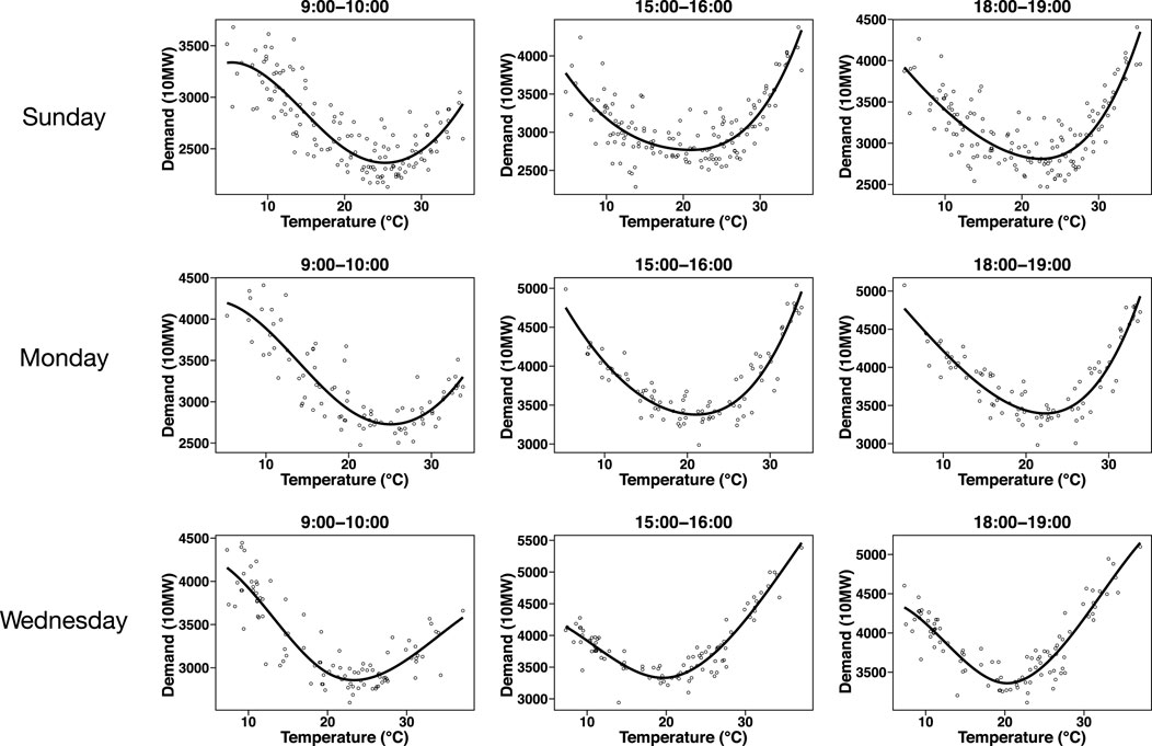
FIGURE 1. Relationship between maximum temperature and demand for different time intervals on Sunday, Monday, and Wednesday. The curves are depicted by fitting the ordinary least squares estimation with the cubic B-spline function.
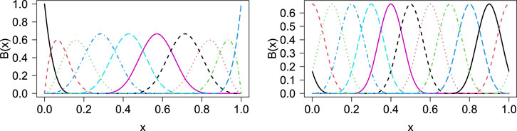
FIGURE 2. B-spline functions of 3 degree (left panel) and cyclic B-spline functions of 3 degree (right panel) with M = 10.
The curve shape for 9:00–10:00 is different from that for 15:00–16:00, which suggests that the regression coefficients must be different among time intervals. Meanwhile, the curve shapes for 15:00–16:00 and 18:00–19:00 are similar. In this case, it is reasonable to assume that the regression coefficients for 15:00–16:00 are similar to those for 18:00–19:00. The regression coefficients are assumed to change depending on the time interval yet to be smooth according to the time interval. To achieve a smooth function of βm(j), we also use the cubic B-spline as a basis function of hq(j). As the ordinary B-spline function cannot produce a smooth curve around the boundary (i.e., 23:00–0:00 and 0:00–1:00), we employ the cyclic B-spline function, where the basis functions wrap at the first and last knot locations. The cyclic B-spline function is implemented in the cSplineDes function in the mgcv package in R. The right panel of Figure 2 shows the cyclic B-spline function of degree 3 with M = 10.
We also observe that the curve shapes are different among each day of the week. Therefore, we construct the statistical models by day of the week separately; seven statistical models are constructed. To forecast the demand, we select a model that matches the day of the week. All national holidays are regarded as Sunday; therefore, the number of observations on Sunday is larger than on other weekdays.
4.2 Candidates of Tuning Parameters
We employ our proposed method based on two estimation procedures: ridge estimation
and NNLS estimation with the ridge penalty in Eq. 12. We label these estimation procedures as “LSE” and “NNLS,” respectively. For both LSE and NNLS, we prepare a wide variety of statistical models by changing the tuning parameters. Here, we review the role of each tuning parameter and present their candidates as follows:
• Q: the number of basis functions in the varying coefficient model. As Q increases, the electricity fluctuations caused by weather becomes large in time interval j (j = 1, … , J). As we will show in Section 4.3, the value of Q may not highly affect the forecast accuracy. Therefore, it would be sufficient to set the candidates of Q as Q = 5, 10.
• M: the number of basis functions for the impact of weather on demand. As M increases, the electricity fluctuations caused by weather becomes large in temperature si. As shown in Figure 1, M = 5 would be sufficient to express the relationship between weather and demand. Therefore, the candidates of M are M = 5, 10.
• T: the number of past demands for forecasting. In other words, we use demand in the past T days to forecast demand. In this numerical analysis, we construct the statistical models by day of the week separately. Therefore, the forecast is done by using the past T weeks on the same day of the week. Consequently, it would be sufficient to set the candidates of T as T = 2, 4.
• λ: regularization parameter for ridge regression. As λ increases, the regression coefficients become stable. Small λ prevents the overfitting, but too large λ leads to large bias. The candidates of λ are 20 sequences from 10–5 to 1.0 on a log-scale. We note that the log-scale sequence is often used to set the candidates of the regularization parameters (e.g., Friedman et al., 2010). We also set λ = 0 to investigate the impact of the ridge parameter on the forecast accuracy. As we will see in Section 4.3, it would be sufficient to set the above candidates of λ to achieve good accuracy.
In addition to the above candidates of models, we consider two types of αjt: sample mean of the past demand (i.e., αjt = 1/T) and AR(1) structure. Details of the AR(1) structure are presented at the end of Section 2.2. As a result, the total number of candidates of the models is 336 (= 2 × 2 × 2 × (20 + 1) × 2). These candidates are summarized in Table 1.
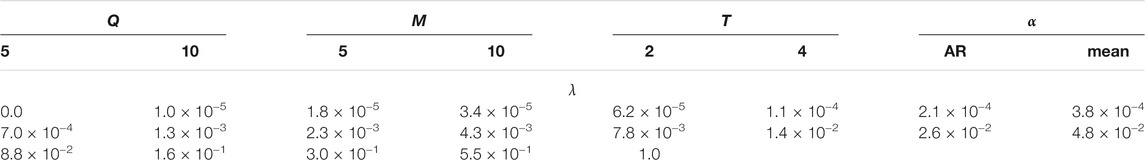
TABLE 1. Candidates of tuning parameters for our proposed method.
4.3 Impact of Tuning Parameters on Forecast Accuracy
The forecast accuracy of our proposed method depends on the tuning parameters presented above. We investigate the impact of tuning parameters on the mean absolute percentage error (MAPE) defined as
Figure 3 shows the relationship between regularization parameter λ and MAPE. The relationships are investigated for all combinations of (Q, M, T).
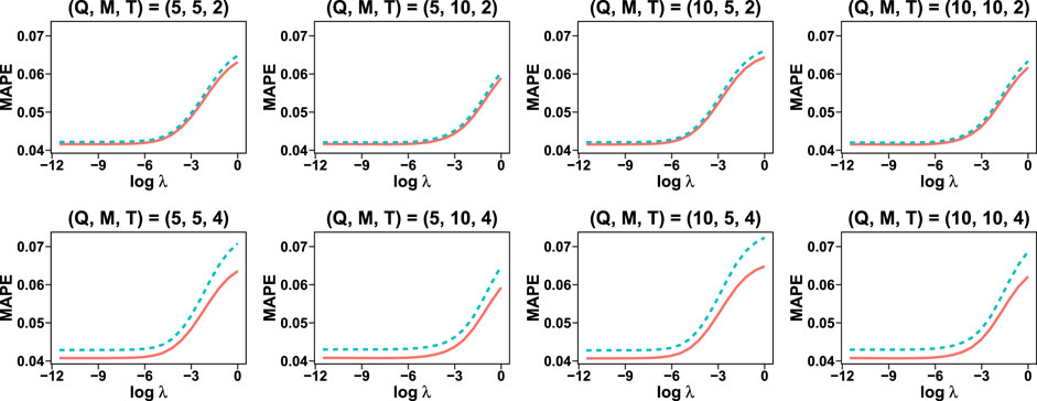
FIGURE 3. Impact of regularization parameter λ on the MAPE, investigated for all combinations of (Q, M, T). The dashed line indicates αjt = 1/T and the solid line corresponds to the AR(1) structure.
The result shows that the AR(1) structure on αjt produces smaller MAPE than the mean structure (αjt = 1/T) for all candidates of ridge parameter λ. For AR(1) model, the performance for T = 4 is better than that for T = 2. We observe that a large value of λ may result in poor forecast accuracy; meanwhile, a small amount of λ generally results in good accuracy. The result for λ = 0 is not displayed here because the MAPE can be extremely large due to the non-convergence of parameters; the ridge penalty helps avoid such a non-convergence. In summary, the AR(1) structure on αjt, T = 4, and a small value of λ will result in a small MAPE for this dataset.
4.4 Forecast Accuracy
We compare the performance of our proposed method with the following popular machine learning techniques: random forest (RF), support vector machine (SVM), Least absolute shrinkage and selection operator (Lasso), LightGBM (LGBM; (Ke et al., 2017)), and Long Short Term Memory [LSTM; (Hochreiter and Schmidhuber, 1997; Van Houdt et al., 2020)]. The RF, SVM, LGBM, and LSTM involve nonlinear functions, allowing us to capture complex structures. We use R packages randomForest, ksvm, glmnet, and lgbm to implement RF, SVM, Lasso, and LGBM, respectively. The LSTM is implemented by tensorflow.keras library in python. The LGBM is based on the gradient boosting decision tree and achieves good forecast accuracy in various fields of research, including energy (e.g., (Ju et al., 2019)). The LSTM is the state-of-the-art technique for analyzing time series data using artificial neural networks (ANN). For these machine learning techniques, the forecast is made by the electricity demand of past T days and maximum temperature, that is,
The characteristics of our proposed method and the machine learning techniques are compared in Table 2.
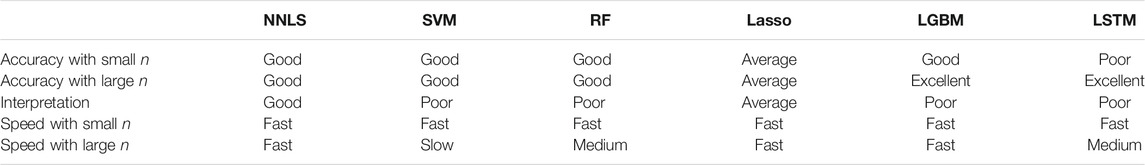
TABLE 2. Characteristics of our proposed method (NNLS) and the state-of-the-art machine learning techniques in terms of forecast accuracy, interpretation, and computational speed.
A detailed description of Table 2 is as follows:
• With small sample sizes, the machine learning methods that capture nonlinear structure provide good accuracy except for the LSTM; in general, the ANN can often yield poor accuracy with small sample sizes (e.g., Tange et al., 2017). The accuracy of the lasso is not sufficiently but relatively high because the lasso cannot capture the nonlinear structure. When the number of observations is large, the LGBM and LSTM will perform perfectly well because these methods capture complex nonlinear structures. However, the sample sizes of the dataset used in this Section (and also other Sections) may not be large.
• Our proposed method is interpretable thanks to the nonlinear regression modeling with basis expansions. The lasso may also be interpretable, but it only captures the linear structure. The other machine learning techniques might not be suitable for interpretation purposes; please refer to Section 4.5 for the numerical results.
• The computational speed of our proposed method turns out to be fast thanks to the efficient NNLS algorithm of Lawson and Hanson (Lawson and Hanson, 1995). The lasso algorithm (Friedman et al., 2010) is also extremely fast. The RF is a little bit slow with large sample sizes due to the resampling procedure. The LGBM is very fast regardless of sample sizes in our experience. The SVM becomes extremely slow with large n (e.g., n = 100,000) because we must compute the Kernel function for each pair of observations, which requires O(n2) operations.
In practice, we need to select a set of tuning parameters among candidates. The candidates of the tuning parameters for the proposed method are presented in Section 4.3. For machine learning methods, the candidates are detailed in Section S3 in the Supplementary Material. For all methods, we must select an appropriate set of tuning parameters. These tuning parameters are generally selected with cross-validation. In this study, we choose these tuning parameters to minimize the MAPE in the past year. The values of tuning parameters are changed every month.
Table 3 shows the monthly MAPE for our proposed method and existing methods from April 2019 to March 2020. The result shows that the proposed method performs better than existing machine learning techniques in total. The SVM achieves the best performance in specific months but sometimes provides much larger MSE than other methods, resulting in worse performance than our proposed method in total. The RF and LGBM yield similar performance, and these methods produce larger MAPE than our proposed method. The lasso cannot capture the nonlinear relationship between temperature and demand as in Figure 1, resulting in poor performance in total. The LSTM provides the worst performance, probably due to the small number of observations: it is from n = 132 to n = 302. In general, the ANN does not perform well with such small sample sizes; (Tange et al., 2017) showed that the ANN performed worse than SVM for small sample sizes, and several similar numerical results are found in the literature (Bećirović and Ćosović, 2016; Dehalwar et al., 2016; Maldonado et al., 2019). We observe that the NNLS and LSE result in similar values of MAPE. These similar results are obtained probably due to the identifiability of the parameter. Our proposed procedure decomposes yt as yt ≈ μt + bt, and this decomposition is not unique. Therefore, the NNLS and LSE produce different values of
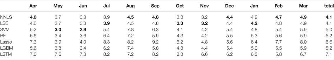
TABLE 3. Monthly MAPE for our proposed methods (NNLS and LSE) and existing machine learning techniques (SVM, RF, Lasso, LGBM, and LSTM) on the dataset from Tokyo Electric Power Company Holdings from April 2019 to March 2020. The smallest MAPE is written in bold.
We also compute the MAPE for well-known Global Energy Forecasting Competition 2014 (GEFCom 2014) data (Hong and Fan, 2016), and obtain a similar result as that shown in Table 3. For detail, please refer to Section S4 in the Supplementary Material.
4.5 Interpretation
With our proposed method, the estimated model can be interpreted by decomposing the forecast value by the effects of temperature and past demand:
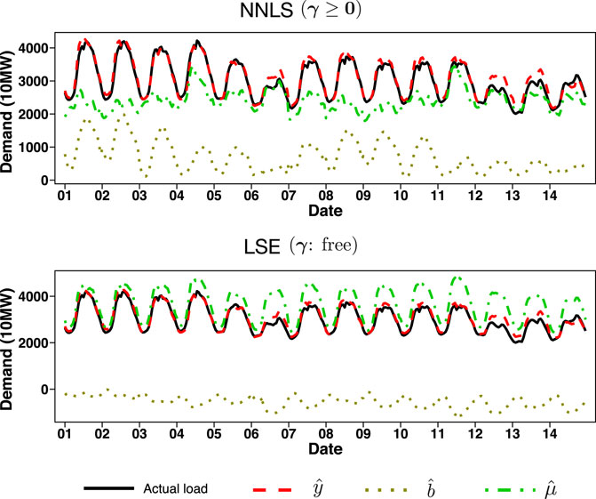
FIGURE 4. The values,
Although the forecast accuracy of the LSE estimation is similar to that of the NNLS estimation, as shown in Table 3, the results of the decomposition
In contrast, the effect of weather is appropriately captured by the NNLS estimation. Indeed, in many cases, the value of
To further investigate the effect of temperature, we depict
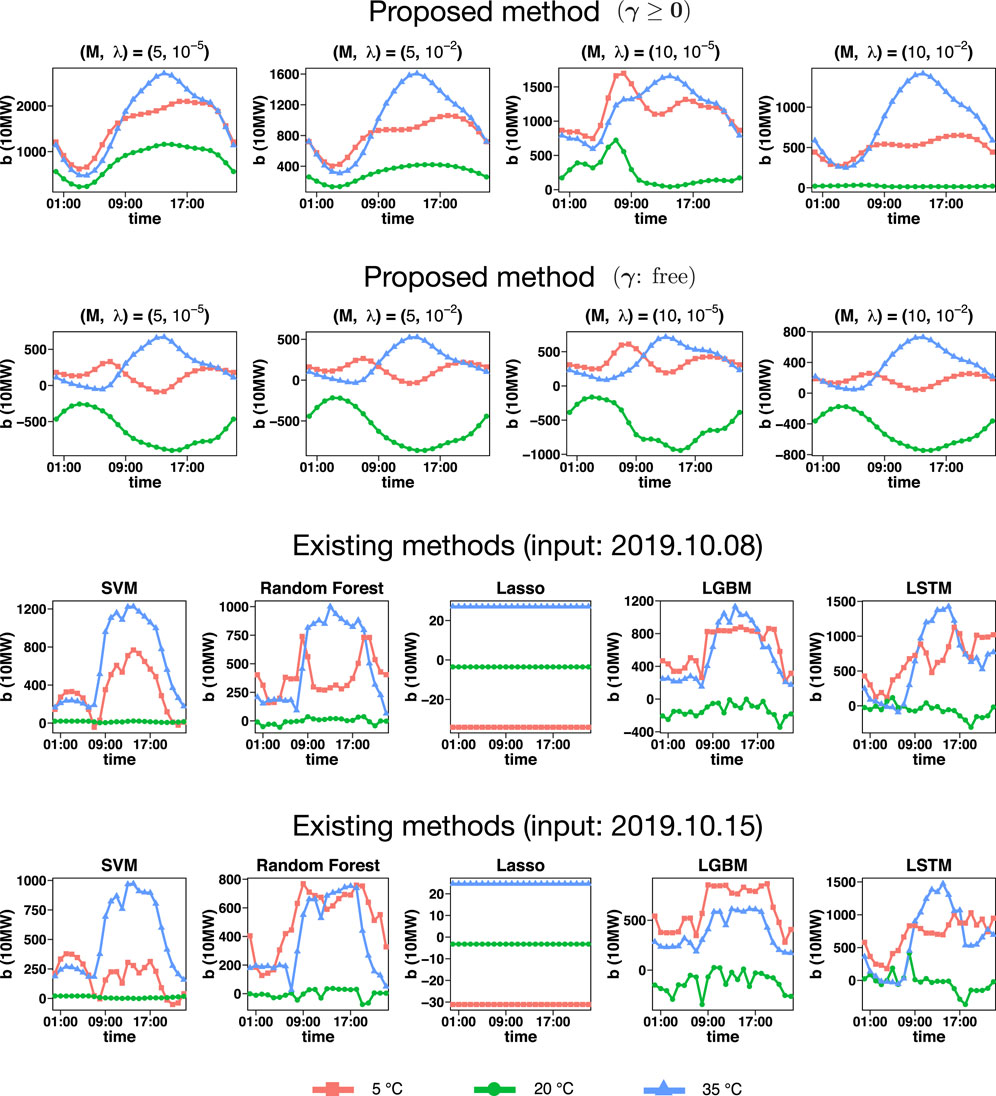
FIGURE 5. Estimate of the weather effect bij on Tuesday for the proposed method and existing methods. For existing methods, the weather effect depends on the input. We depict the weather effect on October 8th, 2019, and October 15th, 2019, for existing methods; both of these days of week are Tuesday
The results of our proposed procedure show that
The existing machine learning methods, RF, SVM, LGBM, and LSTM, are unstable and highly depend on the input. With the Lasso, the impact of temperature is almost zero, which implies that the weather effect cannot be captured. Our proposed method results in smoother curves than existing methods thanks to the B-spline basis expansion of regression coefficients in Eq. 4. As a result, our proposed method is more suitable for interpreting the weather effect than existing methods.
5 Application to Data From One Selected Research Facility in Japan
In the second real data example, we apply our proposed method to the demand data from one selected research facility in Japan. The raw data cannot be published due to confidentiality. This dataset consists of demand from January 1st, 2017 to May 30th, 2020. At certain times, demand is either not observed or include outliers due to electricity meter failures or blackouts. The daily data that contain such missing values and outliers are removed, resulting in 1,164 days of complete data. The demand is shown in kW at 1-h intervals (J = 24).
We observe that COVID-19 greatly influences the usage of this research facility’s electricity pattern due to the recommendation of telework. In present times, it is essential to forecast the demand for this extraordinary situation. To this end, our proposed method is directly applicable to the input of daily data related to COVID-19, and we focus our attention on the forecast accuracy in March, April, and May 2020.
5.1 Input of COVID-19 Information
In Japan, the most frequently-used daily information about COVID-19 is the daily number of infections, available at https://www3.nhk.or.jp/news/special/coronavirus/data-all/. However, this variable turns out to be relatively unstable. In order to use more stable information about COVID-19, we may use the moving average of the number of infections; that is, the average number of infections in the past several days.
The research facility used in this study promotes the staff to work from home to prevent the spread of COVID-19. We expect that the electricity usage of the research facility decreases as the number of infected people of the COVID-19 increases; therefore, the COVID-19 information may affect the forecast results. Figure 6 shows the relationship between the number of daily infections and demand, and between the average number of infections in the past 14 days and demand. We depict these plots on working days. The curve fitting is done by polynomial regression with cubic function. The B-spline may not be suitable in this case due to the limited number of observations.
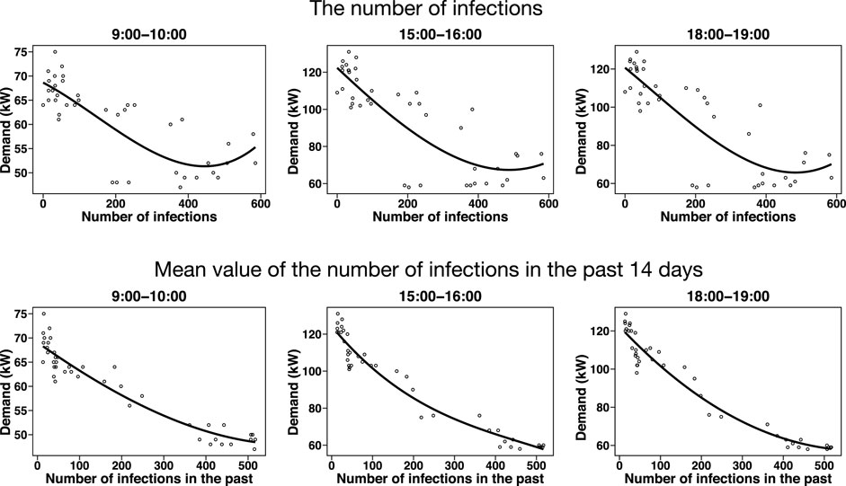
FIGURE 6. Relationship between the number of daily infections and demand (upper panels), and between the average number of infections in the past 14 days and demand (lower panels). We depict these plots on working days. The curve fitting is done by polynomial regression with cubic function.
The number of daily infections includes outliers; thus resulting in unstable curve fitting. For example, when the number of infections is relatively large, the demand increases as the number of infections increases. This phenomenon is counterintuitive because this facility encourages working at home as much as possible to prevent infections. On the other hand, the average number of infections in the past 14 days is negatively correlated with the demand, and the curve fitting of the cubic function works well. For this reason, we use the average number of infections in the past 14 days as daily information about COVID-19. As a result, the daily variable si becomes a two-dimensional vector that consists of the maximum temperature and the average number of infections in the past 14 days. We use the cubic B-spline function as a basis function of maximum temperature, and the cubic function as a basis function of the average number of infections in the past 14 days.
5.2 Forecast Accuracy
In the previous real data example, we construct the statistical models by day of the week separately. However, in this case, the number of observations affected by COVID-19 is excessively small. Thus, only two statistical models are constructed based on working days (from Monday to Friday) and holidays (Saturday, Sunday, and national holidays). We consider the problem of the day-ahead forecast from March 1st, 2020 to May 30th, 2020 (data in 2017–2019 are only used for training). The training data consist of all demand data up to the previous day of the forecast day.
We investigate how the input of COVID-19 information improves the forecast accuracy. The NNLS does not produce negative regression coefficients but we observe that the electricity usage decreases as the average number of infections in the past 14 days increases, as shown in Figure 6. Thus, the electricity fluctuation caused by COVID-19, say
Figure 7 shows the forecast values with our proposed method using NNLS and the actual demand. We depict two forecast values: one uses the information about COVID-19 and the other does not. The result shows that the usage of the COVID-19 data slightly improves the accuracy; for example, on the 10th and 13th.
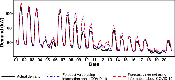
FIGURE 7. Actual demand and forecast values from April 1st, 2020 to April 20th, 2020.
Figure 8 shows
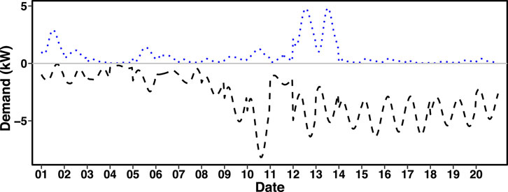
FIGURE 8.
Table 4 shows MAPE for our proposed method and existing methods on March, April, and May 2020. We also compare the performance of two estimation procedures: one uses the information about COVID-19 and the other does not. In March, the result shows that the proposed method performs the best and Lasso yields the worst performance. This is because the effect of temperature can be appropriately captured as shown in the previous example. The effect of COVID-19 is not crucial in March because the performance becomes worse when the COVID-19 information is included.
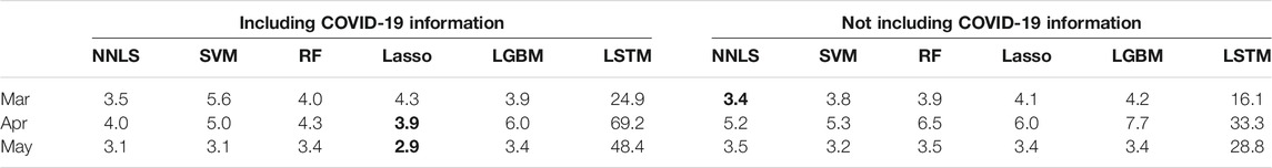
TABLE 4. Monthly MAPE for our proposed methods (NNLS and LSE) and existing machine learning techniques (SVM, RF, Lasso, LGBM, and LSTM) on the dataset from one selected research facility in March, April, and May 2020. The smallest MAPE is written in bold.
In April and May, the information about COVID-19 significantly improves the performance for almost all methods. In particular, our proposed method and Lasso both produce small MAPE values, and interestingly, Lasso performs slightly better than our proposed method. There are two reasons to explain the superiority of Lasso. First, the relationship between the number of infections and the demand is approximated by a linear function, as shown in Figure 6. Second, the temperature effect is not crucial because the temperature does not change much in April and May. The nonlinear machine learning techniques, that is, SVM, RF, LGBM, and LSTM yield large MAPE in April, probably due to the small number of observations related to COVID-19; these techniques result in overfitting. In particular, LSTM produces much worse MAPE than other methods. Such poor results may be due to the instability of the electricity demand; the neural networks can be highly sensitive to noise [e.g., (Goodfellow et al., 2014)]. Indeed, we observe that the electricity demand of this dataset turns out to be unstable compared with the datasets from Tokyo electric power company holdings and Global Energy Forecasting Competition 2014. To improve the accuracy of the LSTM, we need to change the input/output by incorporating much more information of the data (e.g., not daily but hourly weather and hourly COVID-19 data).
6 Concluding Remarks
We have constructed a statistical model for forecasting future electricity demand. To capture the nonlinear effect of weather information, we employed the varying coefficient model. With the ordinary least squares estimation (LSE), the estimate of bij, say
The proposed method is carried out under the assumption that the errors are uncorrelated. In practice, however, the errors among near time intervals may be correlated. As a future research topic, it would be interesting to assume a correlation among time intervals and estimate a regression model that includes the correlation parameter. Another important point is to incorporate the weather effects other than temperature and humidity; we may use cloud cover (Apadula et al., 2012), rainfall, and wind speed (Chapagain and Kittipiyakul, 2018). However, incorporating too many variables can often result in low forecast accuracy due to overfitting (Xie et al., 2016). The selection of an appropriate combination of variables is essential but beyond the scope of this study; we would like to take this as a future research topic.
Recently, demand response has been becoming one of the most important topics in the research field of energy. In particular, the machine learning techniques have been recently used for residential demand response (Zhou et al., 2016; Pallonetto et al., 2019; Afzalan and Jazizadeh, 2020). These techniques are based on the deterministic approaches. On the other hand, our proposed statistical model will lead to the demand response by the probabilistic approach (Schachter and Mancarella, 2015; Alipour et al., 2017). The probabilistic approach will allow the decision based on the probabilistic risk evaluation. Such demand response would be essential in practice, and we would like to work on this topic in the future.
Data Availability Statement
Publicly available datasets were analyzed in this study. This data can be found here: https://www.tepco.co.jp/en/forecast/html/download-e.html https://www.jma.go.jp/jma/indexe.html https://www3.nhk.or.jp/news/special/coronavirus/data-all/ http://blog.drhongtao.com/2017/03/gefcom2014-load-forecasting-data.html.
Author Contributions
The author confirms being the sole contributor of this work and has approved it for publication.
Funding
This work was partially supported by the Japan Society for the Promotion of Science KAKENHI Grant Number JP19K11862 and the Center of Innovation Program (COI) from JST Grant Number JPMJCE1318, Japan.
Conflict of Interest
The author declares that the research was conducted in the absence of any commercial or financial relationships that could be construed as a potential conflict of interest.
Publisher’s Note
All claims expressed in this article are solely those of the authors and do not necessarily represent those of their affiliated organizations or those of the publisher, the editors, and the reviewers. Any product that may be evaluated in this article, or claim that may be made by its manufacturer, is not guaranteed or endorsed by the publisher.
Acknowledgments
The author would like to thank reviewers for the constructive and helpful comments that improved the quality of the paper considerably. The author also thanks Professor Hiroki Masuda and Maiya Hori for helpful comments and discussions.
Supplementary Material
The Supplementary Material for this article can be found online at: https://www.frontiersin.org/articles/10.3389/fenrg.2021.724780/full#supplementary-material
References
Afzalan, M., and Jazizadeh, F. (2020). A Machine Learning Framework to Infer Time-Of-Use of Flexible Loads: Resident Behavior Learning for Demand Response. IEEE Access 8, 111718–111730. doi:10.1109/access.2020.3002155
Alipour, M., Zare, K., and Abapour, M. (2017). Minlp Probabilistic Scheduling Model for Demand Response Programs Integrated Energy Hubs. IEEE Trans. Ind. Inform. 14, 79–88.
Amral, N., Ozveren, C. S., and King, D. (2008). “Short Term Load Forecasting Using Multiple Linear Regression,” in 2007 42nd International Universities Power Engineering Conference (IEEE), 1192–1198.
Apadula, F., Bassini, A., Elli, A., and Scapin, S. (2012). Relationships between Meteorological Variables and Monthly Electricity Demand. Appl. Energ. 98, 346–356. doi:10.1016/j.apenergy.2012.03.053
Bećirović, E., and Ćosović, M. (2016). “Machine Learning Techniques for Short-Term Load Forecasting,” in 2016 4th International Symposium on Environmental Friendly Energies and Applications (EFEA) (IEEE), 1–4. doi:10.1109/efea.2016.7748789
Bedi, J., and Toshniwal, D. (2019). Deep Learning Framework to Forecast Electricity Demand. Appl. Energ. 238, 1312–1326. doi:10.1016/j.apenergy.2019.01.113
Bro, R., and De Jong, S. (1997). A Fast Non-negativity-constrained Least Squares Algorithm. J. Chemometrics 11, 393–401. doi:10.1002/(sici)1099-128x(199709/10)11:5<393:aid-cem483>3.0.co;2-l
Cabrera, B. L., and Schulz, F. (2017). Forecasting Generalized Quantiles of Electricity Demand: A Functional Data Approach. J. Am. Stat. Assoc. 112, 127–136. doi:10.1080/01621459.2016.1219259
Chapagain, K., and Kittipiyakul, S. (2018). Performance Analysis of Short-Term Electricity Demand with Atmospheric Variables. Energies 11, 818. doi:10.3390/en11040818
Chen, Y., Xu, P., Chu, Y., Li, W., Wu, Y., Ni, L., et al. (2017). Short-term Electrical Load Forecasting Using the Support Vector Regression (SVR) Model to Calculate the Demand Response Baseline for Office Buildings. Appl. Energ. 195, 659–670. doi:10.1016/j.apenergy.2017.03.034
De Boor, C. (1972). On Calculating with B-Splines. J. Approximation Theor. 6, 50–62. doi:10.1016/0021-9045(72)90080-9
de Oliveira, E. M., and Cyrino Oliveira, F. L. (2018). Forecasting Mid-long Term Electric Energy Consumption through Bagging ARIMA and Exponential Smoothing Methods. Energy 144, 776–788. doi:10.1016/j.energy.2017.12.049
Dehalwar, V., Kalam, A., Kolhe, M. L., and Zayegh, A. (2016). “Electricity Load Forecasting for Urban Area Using Weather Forecast Information,” in 2016 IEEE International Conference on Power and Renewable Energy (ICPRE) (IEEE), 355–359. doi:10.1109/icpre.2016.7871231
Dudek, G. (2016). Pattern-based Local Linear Regression Models for Short-Term Load Forecasting. Electric Power Syst. Res. 130, 139–147. doi:10.1016/j.epsr.2015.09.001
Engle, R. F., Granger, C. W. J., Rice, J., and Weiss, A. (1986). Semiparametric Estimates of the Relation between Weather and Electricity Sales. J. Am. Stat. Assoc. 81, 310–320. doi:10.1080/01621459.1986.10478274
Fan, J. Q., and Zhang, W. Y. (1999). Statistical Estimation in Varying Coefficient Models. Ann. Stat. 27, 1491–1518. doi:10.1214/aos/1017939139
Franc, V., Hlaváč, V., and Navara, M. (2005). Sequential Coordinate-wise Algorithm for the Non-negative Least Squares Problem. Comp. Anal. Images Patterns, Proc. 3691, 407–414. doi:10.1007/11556121_50
Friedman, J., Hastie, T., and Tibshirani, R. (2010). Regularization Paths for Generalized Linear Models via Coordinate Descent. J. Stat. Softw. 33, 1–22. doi:10.18637/jss.v033.i01
Goodfellow, I. J., Shlens, J., and Szegedy, C. (2014). Explaining and Harnessing Adversarial Examples. arXiv preprint arXiv:1412.6572.
Guo, Z., Zhou, K., Zhang, C., Lu, X., Chen, W., and Yang, S. (2018). Residential Electricity Consumption Behavior: Influencing Factors, Related Theories and Intervention Strategies. Renew. Sustain. Energ. Rev. 81, 399–412. doi:10.1016/j.rser.2017.07.046
Guo, Z., Zhou, K., Zhang, X., and Yang, S. (2018). A Deep Learning Model for Short-Term Power Load and Probability Density Forecasting. Energy 160, 1186–1200. doi:10.1016/j.energy.2018.07.090
Haq, M. R., and Ni, Z. (2019). A New Hybrid Model for Short-Term Electricity Load Forecasting. IEEE Access 7, 125413–125423. doi:10.1109/access.2019.2937222
Harvey, A., and Koopman, S. J. (1993). Forecasting Hourly Electricity Demand Using Time-Varying Splines. J. Am. Stat. Assoc. 88, 1228–1236. doi:10.1080/01621459.1993.10476402
Hastie, T., Tibshirani, R., and Friedman, J. (2008). The Elements of Statistical Learning. 2nd edn. New York: Springer.
Hastie, T., and Tibshirani, R. (1993). Varying-Coefficient Models. J. R. Stat. Soc. Ser. B (Methodological) 55, 757–779. doi:10.1111/j.2517-6161.1993.tb01939.x
He, W. (2017). Load Forecasting via Deep Neural Networks. Proced. Comp. Sci. 122, 308–314. doi:10.1016/j.procs.2017.11.374
Hochreiter, S., and Schmidhuber, J. (1997). Long Short-Term Memory. Neural Comput. 9, 1735–1780. doi:10.1162/neco.1997.9.8.1735
Hoerl, A. E., and Kennard, R. W. (1970). Ridge Regression: Biased Estimation for Nonorthogonal Problems. Technometrics 12, 55–67. doi:10.1080/00401706.1970.10488634
Hong, T., and Fan, S. (2016). Probabilistic Electric Load Forecasting: A Tutorial Review. Int. J. Forecast. 32, 914–938. doi:10.1016/j.ijforecast.2015.11.011
Hong, T., Gui, M., Baran, M. E., and Willis, H. L. (2010). Modeling and Forecasting Hourly Electric Load by Multiple Linear Regression with Interactions. IEEE PES Gen. Meet., 1–8. doi:10.1109/pes.2010.5589959
Jiang, H., Zhang, Y., Muljadi, E., Zhang, J. J., and Gao, D. W. (2018). A Short-Term and High-Resolution Distribution System Load Forecasting Approach Using Support Vector Regression with Hybrid Parameters Optimization. IEEE Trans. Smart Grid 9, 3341–3350. doi:10.1109/tsg.2016.2628061
Ju, Y., Sun, G., Chen, Q., Zhang, M., Zhu, H., and Rehman, M. U. (2019). A Model Combining Convolutional Neural Network and Lightgbm Algorithm for Ultra-short-term Wind Power Forecasting. IEEE Access 7, 28309–28318. doi:10.1109/access.2019.2901920
Ke, G., Meng, Q., Finley, T., Wang, T., Chen, W., Ma, W., et al. (2017). “Lightgbm: A Highly Efficient Gradient Boosting Decision Tree,” in Advances in Neural Information Processing Systems, 3146–3154.
Kong, W., Dong, Z. Y., Jia, Y., Hill, D. J., Xu, Y., and Zhang, Y. (2018). Short-Term Residential Load Forecasting Based on LSTM Recurrent Neural Network. IEEE Trans. Smart Grid 10, 841–851.
Lawson, C. L., and Hanson, R. J. (1995). Solving Least Squares Problems. Philadelphia, PA: Society for Industrial and Applied Mathematics. doi:10.1137/1.9781611971217 Solving Least Squares Problems.
Lee, J. D., Sun, D. L., Sun, Y., and Taylor, J. E. (2016). Exact post-selection Inference, with Application to the Lasso. Ann. Stat. 44, 907–927. doi:10.1214/15-aos1371
Lee, J. D., and Taylor, J. E. (2014). Exact Post Model Selection Inference for Marginal Screening. arXiv.1402, 5596.
Liu, B., Nowotarski, J., Hong, T., and Weron, R. (2017). Probabilistic Load Forecasting via Quantile Regression Averaging on Sister Forecasts. IEEE Trans. Smart Grid 8, 730–737.
Lundberg, S. M., and Lee, S.-I. (2017). “A Unified Approach to Interpreting Model Predictions,” in Advances in Neural Information Processing Systems, 4765–4774.
Lusis, P., Khalilpour, K. R., Andrew, L., and Liebman, A. (2017). Short-term Residential Load Forecasting: Impact of Calendar Effects and Forecast Granularity. Appl. Energ. 205, 654–669. doi:10.1016/j.apenergy.2017.07.114
Maldonado, S., González, A., and Crone, S. (2019). Automatic Time Series Analysis for Electric Load Forecasting via Support Vector Regression. Appl. Soft Comput. 83, 105616. doi:10.1016/j.asoc.2019.105616
Miswan, N. H., Said, R. M., and Anuar, S. H. H. (2016). ARIMA with Regression Model in Modelling Electricity Load Demand. J. Telecommunication, Electron. Comp. Eng. 8, 113–116.
Pallonetto, F., De Rosa, M., Milano, F., and Finn, D. P. (2019). Demand Response Algorithms for Smart-Grid Ready Residential Buildings Using Machine Learning Models. Appl. Energ. 239, 1265–1282. doi:10.1016/j.apenergy.2019.02.020
Ribeiro, M. T., Singh, S., and Guestrin, C. (2016). ““Why Should I Trust You?” Explaining the Predictions of Any Classifier,” in Proceedings of the 22nd ACM SIGKDD international conference on knowledge discovery and data mining, 1135–1144.
Ruiz-Abellón, M. C., Fernández-Jiménez, L. A., Guillamón, A., Falces, A., García-Garre, A., and Gabaldón, A. (2020). Integration of Demand Response and Short-Term Forecasting for the Management of Prosumers’ Demand and Generation. Energies 13, 11.
Saber, A. Y., and Alam, A. K. M. R. (2017). “Short Term Load Forecasting Using Multiple Linear Regression for Big Data,” in 2017 IEEE Symposium Series on Computational Intelligence (SSCI), 1–6. doi:10.1109/SSCI.2017.8285261
Schachter, J. A., and Mancarella, P. (2015). Demand Response Contracts as Real Options: a Probabilistic Evaluation Framework under Short-Term and Long-Term Uncertainties. IEEE Trans. Smart Grid 7, 868–878. doi:10.1109/tsg.2015.2405673
Tange, R. I., Rasmussen, M. A., Taira, E., and Bro, R. (2017). Benchmarking Support Vector Regression against Partial Least Squares Regression and Artificial Neural Network: Effect of Sample Size on Model Performance. J. Near Infrared Spectrosc. 25, 381–390. doi:10.1177/0967033517734945
Timotheou, S. (2016). Fast Non-negative Least-Squares Learning in the Random Neural Network. Prob. Eng. Inf. Sci. 30, 379–402. doi:10.1017/s0269964816000061
Van Houdt, G., Mosquera, C., and Nápoles, G. (2020). A Review on the Long Short-Term Memory Model. Artif. Intell. Rev. 53, 5929–5955. doi:10.1007/s10462-020-09838-1
Vilar, J., Aneiros, G., and Raña, P. (2018). Prediction Intervals for Electricity Demand and price Using Functional Data. Int. J. Electr. Power Energ. Syst. 96, 457–472. doi:10.1016/j.ijepes.2017.10.010
Wang, F., Liu, L., Yu, Y., Li, G., Li, J., Shafie-Khah, M., et al. (2018). Impact Analysis of Customized Feedback Interventions on Residential Electricity Load Consumption Behavior for Demand Response. Energies 11, 770. doi:10.3390/en11040770
Wang, Y., Gan, D., Sun, M., Zhang, N., Lu, Z., and Kang, C. (2019). Probabilistic Individual Load Forecasting Using Pinball Loss Guided Lstm. Appl. Energ. 235, 10–20. doi:10.1016/j.apenergy.2018.10.078
Xie, J., Chen, Y., Hong, T., and Laing, T. D. (2016). Relative Humidity for Load Forecasting Models. IEEE Trans. Smart Grid 9, 191–198.
Yang, A., Li, W., and Yang, X. (2019). Short-term Electricity Load Forecasting Based on Feature Selection and Least Squares Support Vector Machines. Knowledge-Based Syst. 163, 159–173. doi:10.1016/j.knosys.2018.08.027
Zhang, N., Li, Z., Zou, X., and Quiring, S. M. (2019). Comparison of Three Short-Term Load Forecast Models in Southern california. Energy 189, 116358. doi:10.1016/j.energy.2019.116358
Keywords: basis expansion, nonnegative least squares (NNLS), short-term demand forecasting, varying coefficient model (VCM), COVID-19
Citation: Hirose K (2021) Interpretable Modeling for Short- and Medium-Term Electricity Demand Forecasting. Front. Energy Res. 9:724780. doi: 10.3389/fenrg.2021.724780
Received: 14 June 2021; Accepted: 01 November 2021;
Published: 14 December 2021.
Edited by:
Fei Teng, Imperial College London, United KingdomReviewed by:
Ekanki Sharma, University of Klagenfurt, AustriaMd. Abdur Razzak, Independent University, Bangladesh, Bangladesh
Chaoyu Dong, Imperial College London, United Kingdom
Copyright © 2021 Hirose. This is an open-access article distributed under the terms of the Creative Commons Attribution License (CC BY). The use, distribution or reproduction in other forums is permitted, provided the original author(s) and the copyright owner(s) are credited and that the original publication in this journal is cited, in accordance with accepted academic practice. No use, distribution or reproduction is permitted which does not comply with these terms.
*Correspondence: Kei Hirose, aGlyb3NlQGltaS5reXVzaHUtdS5hYy5qcA==