 Zehua Zhao
 Fengji Luo
 Yongxi Zhang
 Gianluca Ranzi1
- 1School of Civil Engineering, The University of Sydney, Sydney, NSW, Australia
- 2School of Electrical and Information Engineering, Changsha University of Science and Technology, Changsha, China
With the prevalence of building automation and Internet-of-Things technologies, home energy management has become an active area in recent years. This paper proposes an integrated, multi-objective Home Energy Management System (HEMS), which optimally schedules controllable electric household appliances to balance three objectives: 1) home energy cost; 2) the occupant’s use satisfaction of controllable appliances; and 3) the occupant’s thermal comfort. In particular, the HEMS models the coupling operational relationship between the non-thermostatically controlled appliances and the air conditioner by investigating the impact of heat gains released by the appliances on the indoor temperature. An advanced multi-objective optimizer is applied to solve the home energy management model. Simulations are conducted to validate the proposed method.
Introduction
Modern buildings are characterized by the penetration of renewable energy sources, Internet-of-Things (IoT) facilities, and building automation technologies. These have been driving buildings transition from static civil infrastructures to be complex cyber-physical entities that are capable of actively interacting with external physical systems, e.g., smart grids. In particular, the demand response (DR) flexibility of buildings (Mathieu et al., 2011), which refers to reducing or shifting building’s energy consumption subjected to grid-side incentive and/or pricing signals, has been recognized as an affordable way for accommodating renewable energy and deferring the grid’s infrastructure investment.
The advances of automation technologies in residential buildings drive the research and development of home energy management systems (HEMSs) (Inoue et al., 2003). A HEMS is an expert system that provides decision-making support to the occupant on scheduling and controlling household energy resources, such as rooftop photovoltaic solar panels and wind turbines, controllable appliances, energy storage devices, and plug-in electric vehicles. Depending on the managed objects, HEMSs can have different designs, which have been extensively studied in the literature. The following are some representative ones: Some research efforts and industrial demonstrations study the operation strategy for home energy storage devices, mainly including battery energy storage systems (BESSs) (Zhang et al., 2020) and the batteries in plug-in electric vehicles (known as the “vehicle-to-home” integration (Liu et al., 2013)). These efforts optimize battery’s charging/discharging power to accommodate the residential renewable energy and provide energy to the household locally. For example, Iwafune et al. (2015) designed a rule-based controller to determine the charging/discharging power of residential BESSs based on the real-time power output of the rooftop photovoltaic (PV) solar panel. The Nissan Motor Company Ltd. demonstrated its “Smart Home of the Future concept” by using a Nissan Leaf vehicle to supply electricity to a house while operating off the power grid (Hornyak, 2011). Some literature study the energy management of air conditioning systems. For example, Jo et al. (2013) propose a coordinated scheduling method for a home BESS and an air conditioning system, aiming at minimizing the household’s energy cost (both electricity cost and gas cost) while maintaining an acceptable indoor thermal comfort level. Dorokhova et al. (2020) propose an occupancy-based air conditioner (AC) control method. It firstly applies machine learning techniques to infer the room’s occupancy from the smart meter data profile. Based on the occupancy state and the building’s heat load, the work designs a rule-based controller to decide the ON/OFF state and operation mode (i.e., heating mode or cooling mode) of the AC.
The increasing prevalence of building IoT devices further lays a foundation to automatically control a wider range of household appliances besides the AC and energy storage systems. Such appliance scheduling methodologies have been actively studied in the literature in recent years. Jindal et al. (2020) propose a heuristic-based scheduling method which schedules both the time shiftable and interruptible appliances in a smart home environment to accommodate the power output of the rooftop PV solar panel and minimize the home net-load. Zhao et al. (2013) optimally schedule a residential BESS and a group of controllable household appliances to maximize the utilities of the appliances to the occupant while reducing the home’s energy cost when subjected to a time-varying electricity tariff. (Ozturk et al. (2013) propose a HEMS, which dynamically schedules appliances in each dwelling unit based on the power demand of the whole community which was forecasted and reported to the utility to make day-ahead grid operation plans. In the authors’ previous work (Luo et al., 2018), a coordinated scheduling model is proposed, which coordinately makes operation plans for an AC, a group of plug-in time shiftable appliances, and a plug-in EV. The authors also develop a multi-stage HEMS (Luo et al., 2019), which schedules a residential BESS and multiple controllable appliances in a PV solar power-penetrated home environment: in the day-ahead forecasting stage, an artificial neural network-based forecasting system is developed to predict the PV solar power output; in the day-ahead scheduling stage, a scheduling model is formulated to determine the BESS’s charging/discharging plan and the appliances’ operation plans; in the actual operation stage, a predictive control-based model is applied to real-time update the charging/discharging actions of the BESS and the appliances’ operation states.
When designing HEMSs, the occupant’s dwelling satisfaction is one of the primary considerations. While the occupant’s satisfaction is a general concept that can be measured in various aspects, two satisfaction categorizes are commonly considered in a typical home environment: (i) usage satisfaction for the household appliances (except for the AC), which is directly related to the appliances’ operation time and/or power consumptions; and (ii) indoor thermal comfort, which is influenced by the indoor air temperature, and the indoor temperature is affected by the outdoor climate and the AC’s operation. These two aspects of satisfaction have been addressed in the state-of-the-art HEMS designs. For the usage satisfaction for typical time shiftable appliances (i.e., the appliances whose operation time is deferrable), it is usually reflected in the constraints that strictly restrict each appliance to operate in an allowable time range that is pre-specified by the occupant (Rastegar et al., 2012; Zhao et al., 2013; Luo et al., 2019). For indoor thermal comfort, the most commonly practiced approach is to control the AC to ensure the indoor temperature within a pre-specified comfort band (Jo et al., 2013; Dorokhova et al., 2020). These approaches can be considered to be “rigorous”, as they use rigid constraints to restrict the appliance’s operation.
Such a rigorous dwelling satisfaction modeling approach shows a major limitation in accurately representing the occupant’s satisfaction. For example, if the occupant sets up an allowable time range for a washing machine (say, 2–8 pm), will the occupant really feel unsatisfied if the washing machine is scheduled to complete its task at 8:01 pm? To overcome the limitation, some research (e.g., the authors’ previous work (Luo F. J. et al., 2017)) proposes linear models to model the relationship between the variation of the occupant’s satisfaction and the deviation between the schedules of the appliances determined by the HEMS and the ones desired by the occupant. But a recent small-scale survey carried out by the authors on three Australian households indicates that the residents’ satisfaction on the appliances’ task completion time follows a non-linear pattern. The residents are asked to provide their subjective satisfaction feeling on the operation of several major household appliances (washing machine, dish washer, clothes dryer, and lighting bulbs). Their feedback is intuitive: if a deferrable appliances’ actual task completion time (or a bulb’s brightness) is close to the desired one, the residents feel it is acceptable; however, their dissatisfaction rapidly increases with the increase of the deviation between the actual and desired task completion time (or bulb’s brightness). This indicates that nonlinear models are more desirable for modeling the occupant’s dwelling satisfaction on appliance operations.
The issue of “rigorous dwelling satisfaction modeling” is also seen in controlling AC systems to maintain the occupant’s thermal comfort. The literature usually uses the “temperature dead band” approach to strictly control the indoor temperature within a pre-specified comfort range of
In addition, there is another limitation that can be identified in the literature. When determining control strategies for the AC, the internal heat gain produced in the building environment is usually considered as a constant parameter (e.g., (Jo et al., 2013)). However, this approach can hardly be applied to HEMS designs where the AC is scheduled with other household appliances. This is because many appliances release heat in their operations. Different schedules of appliances would lead to different temporal variations of their heat gain productions, which would affect the indoor temperature variation and subsequentially influence the AC’s operation. To the best of the authors’ knowledge, coordinately scheduling the AC and other household appliances by considering the appliances’ heat gains is never considered in the existing HEMS designs.
Based on the above discussion, the main contribution of this study is to develop a new HEMS that is centered on an integrated scheduling model for a group of controllable household appliances. The controllable appliances include an AC, multiple time shiftable appliances (TSAs), and multiple power adjustable appliances (PAAs). To overcome the aforementioned limitations of the existing work, the HEMS incorporates a new occupant satisfaction representation method, which uses nonlinear models and adjustable parameters to represent the occupant’s comfort degree when subject to the operation of the different categories of appliances. Further, the developed HEMS links the heat gain produced by the appliances’ operations with the building’s thermal model to implement integrated scheduling for the AC and other appliances by simultaneously considering the household’s energy performance and the occupant’s dwelling satisfaction. In this study, we deliberately do not consider the penetration of energy storage systems and renewable power. This makes the proposed HEMS applicable for many apartment units where these devices are not available. Meanwhile, the models of renewable power sources and energy storage systems can be easily integrated into the proposed HEMS without significant modifications (e.g., following the modeling methodology in our previous work (Luo et al., 2018, 2019)).
This paper is organized as follows. Modeling of Home Energy Resources presents the modeling methodology of home energy resources managed by the HEMS. Modelling of Occupant’s Dwelling Satisfaction and Formulation of Home Energy Management Model present the proposed occupant satisfaction models and the HEMS, respectively. Solving Approach presents the solving approach. Simulation Study discusses the numerical simulation result. Finally, the conclusion is drawn in Conclusion and Future Work.
Modeling of Home Energy Resources
Figure 1 illustrates the operational environment of the HEMS. In this study, we consider that the HEMS manages three types of controllable appliances that are typically seen in current home environments: 1) multiple time shiftable appliances (TSAs, or known as deferrable appliances), whose power consumptions are constant, but operation time can be shifted to a certain extent. Typical appliances in this category include washing machines, clothes dryers, etc.; (b) multiple power adjustable appliances (PAAs), whose operation time is fixed, depending on the occupant’s life requirements; but their power consumptions can be adjusted to a certain extent. Typical appliances in this category include lights, amplifiers, etc.; and (c) an AC, whose operation is driven by the indoor air temperature and the occupant’s thermal comfort preference.
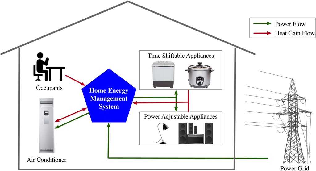
FIGURE 1. Illustration of the HEMS.
Denoting there are a total of
Modeling of Time Shiftable Appliances
Time shiftable appliances represent the appliances whose operation time can be shifted to an extent. Considering there are a total of
1) Operating power (
2) Task duration (
3) Desired task completion time (
4) Heat gain value (
Therefore, each TSA can be modeled as a 4-turple vector:
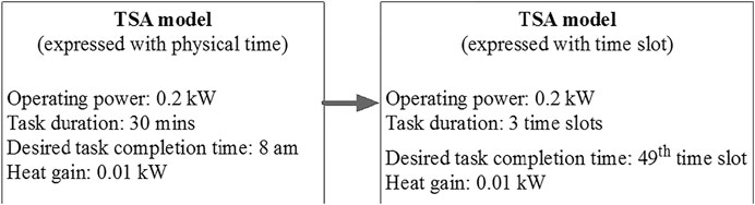
FIGURE 2. Illustration of a TSA model (considering that the scheduling period starts from 7:30 am and the duration of each time slot is 10 min).
Modeling of Power Adjustable Appliances
Considering there are
1) Operation time. Each PAA is associated with one or multiple occupant-specified time points when it is requested to run. The operation time can be represented as a vector
2) Desired power consumption. For each PAA, there is an occupant-specified desirable power consumption value at each operation time point, denoted as
3) Adjustable power range. Each PAA has a lowest power level, denoted as
4) Heat gain value (
Based on the properties mentioned above, Figure 3 provides an example to illustrate the model representation of a PAA.

FIGURE 3. Illustration of a PAA model.
Model of Air Conditioner
The operation of AC is directly related to the room’s thermal model. This section presents the room’s thermal model and the AC’s operation model.
Room’s Thermal Model
There are a number of models in the literature that can be used to model the room’s thermal transition process. In this study, we follow the building thermal model in Ryder-Cook (2009). This thermal model has also been used in other literature about AC energy management (e.g., (Ding et al., 2019)). With this model, the indoor temperature trajectory of the room is described as:
The heat gain
For air-sourced ACs, COP is mainly related to the indoor and outdoor temperature difference and can be approximately expressed as a linear equation:
where
where the function
The heat loss of the room is estimated based on the losses through the building envelope and air leakages (Ryder-Cook, 2009):
Operation Model of Air Conditioner
The operation of the AC is driven by the indoor temperature and the occupant’s thermal comfort preference that is presented in Modelling of Occupant’s Dwelling Satisfaction. The AC has two states: operation state and standby state. Denoting the AC’s state at time
The positive value of
Modeling of Occupant’s Dwelling Satisfaction
Given a schedule of the home energy resources, this study evaluates the occupant’s dwelling satisfaction in three aspects as follows.
Modeling of Occupant’s Satisfaction on Time Shiftable Appliances
For the schedule of the
where the function
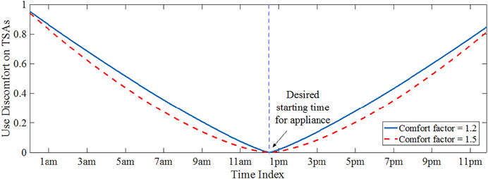
FIGURE 4. Illustration of the occupant’s varying dissatisfaction degree on the operation of a TSA (settings:
Modeling of Occupant’s Satisfaction on Power Adjustable Appliances
For the schedule of the
As an example, Figure 5 plots the occupant’s dissatisfaction degree for a PAA at one time slot subjected to
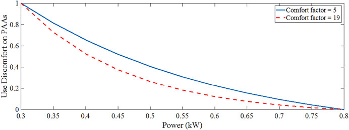
FIGURE 5. Illustration of the variation of the occupant’s dissatisfaction degree on a PAA’s operation at one time slot (
Indoor Thermal Comfort Model for the Occupant
Indoor thermal comfort is an important aspect of the occupant’s dwelling satisfaction. It has a direct relationship with the indoor temperature. Distinguished from many literature papers that set up a rigorous indoor temperature band, we propose to evaluate the occupant’s thermal comfort using the following nonlinear function:
where
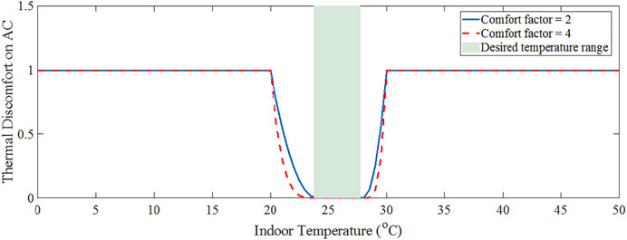
FIGURE 6. Illustration of the variation of the occupant’s discomfort degree on the AC’s operation (
As mentioned in the introduction section, the proposed nonlinear satisfaction models (the ones presented in Modelling of Occupant’s Satisfaction on Time Shiftable Appliances–Indoor Thermal Comfort model for the Occupant) can better represent the nonlinear variation of the occupant’s dissatisfaction. The proposed models also incorporate adjustable satisfaction parameters (
Formulation of Home Energy Management Model
Based on the home energy resources models and occupant comfort models presented in Modelling of Home Energy Resources and Modelling of Occupant’s Dwelling Satisfaction, this section formulates the home energy management model. The model is formulated as a 3-objective optimization problem, in which the HEMS determines the schedules of the controllable appliances to balance the three aspects of considerations in a smart home environment: (i) the home energy cost; (ii) the occupant’s use satisfaction for TSAs and PAAs; and (iii) the occupant’s indoor thermal comfort.
The decision variables of the home energy management model include: (i) start operation time of each TSA, i.e.,
Objective 1—Minimization of the household energy cost:
Objective 2—Minimization of the Occupant’s Use Dissatisfaction for TSAs and PAAs:
Objective 3—Minimization of the Occupant’s Thermal Discomfort:
The home energy management model Eqs. 16-20 is subjected to the following operational constraints:
Constraint (Eq. 21) restricts the adjustable power range of each PAA at each of its operational time slots. Constraint (Eq. 22) ensures that each TSA can only be in the “ON” state in its task execution period. Constraint (Eq. 23) ensures that each PAA does not consume power except at its operational time slot.
Solving Approach
The proposed home energy management model (Modelling of Home Energy Resources–Formulation of Home Energy Management Model) is a mixed-integer, nonlinear multi-objective optimization problem over a finite time horizon. Evolutionary computation has been proved to be an effective technique for solving multi-objective optimization problems and obtaining the Pareto Frontier. In this study, we apply the Multi-Objective Natural Aggregation Algorithm (MONAA) previously proposed by the authors (Luo et al., 2016) to solve the proposed model. MONAA roots from the Natural Aggregation Algorithm (Luo F. et al., 2017)—a swarm-based heuristic algorithm. MONAA mimics group living animals’ self-aggregation intelligence by distributing a group of candidate solutions (called “individuals”) into multiple sub-populations and using a biology-rooted stochastic migration model to migrate the individuals among the sub-populations. It also designs heuristic searching rules to produce mutants of the individuals to search for the global/near global optimal solution in the high dimensional problem space.
The major reasons of using MONAA to solve the proposed home energy management model are two-fold: firstly, by inheriting NAA’s stochastic searching mechanism, MONAA shows satisfactory performance in finding the Pareto Frontier of several engineering optimization problems (e.g., Luo F. et al., 2017; Deng et al., 2020); secondly, the authors have developed a well-packaged MONAA solver, which can be easily interfaced to demand side optimization models. The well-defined interfaces mean the solver can be efficiently and conveniently applied to the proposed home energy management model. Since the optimization algorithm itself is not the primary focus of this paper, other multi-objective optimizers (such as NSGA-II) can also be applied to solve the proposed model with little modifications to the proposed system.
Encoding Scheme
In MONAA, each individual is encoded as a vector with the dimensionality of
1) The first
2) the next
3) the last
Solving Workflow
The solving workflow is shown in Figure 7. Firstly, the models of the appliances (TSAs, PAAs, and the AC), the room model, the occupant satisfaction models, the electricity tariff data, and the predicted outdoor air temperature profile are inputted into the system. Then, MONAA initializes a population of individuals and iteratively produce mutants to perform heuristic searching. After the maximum generation time is reached, the algorithm outputs a set of non-dominated individuals (called the Pareto Frontier).
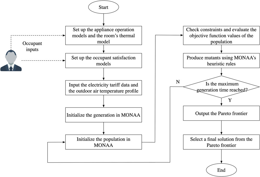
FIGURE 7. Solving workflow for the proposed HEMS.
Since the solutions in the Pareto Frontier are non-dominated with each other, it is unreasonable to say which solutions are “better”; they just represent different compromises of the three optimization objectives. Choosing the final solution from the Pareto Frontier can be completely based on the user’s subjective preference, or can be generated based on certain criteria. The latter approach is useful especially when the number of solutions in the Pareto Frontier is large, which would mean the user would find it difficult to choose. In Simulation Study of this paper, we will discuss the final solution that is selected by a compromise-solution method (Marler and Arora, 2004), shown in Eqs. 24, 25:
where
Simulation Study
This section reports the numerical simulation that is conducted for validating the proposed HEMS. All the programs are implemented on Matlab and are executed on a PC with macOS Catalina, Intel Core i9, with 16 GB memory.
Simulation Setup
We consider a home energy management scenario on a typical cold winter day, where the AC operates in heating mode. The profiles of 1-day solar radiation and outdoor air temperature (Figure 8) are based on the meteorological data of Zhengzhou City, China on a day in March 2021, collected from the “Weather” application on iPhone. The profile of the room’s internal heat gain due to the occupant’s activity is shown in Figure 9, based on the data provided in Heat Gain from People, Lights, and Appliances. The parameters of the room’s thermal model and AC are set as Table 1.
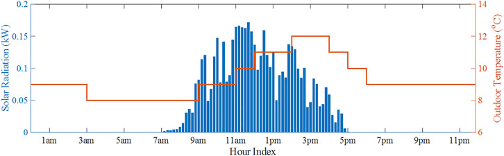
FIGURE 8. Profiles of outdoor temperatures and solar radiation in a typical winter day.
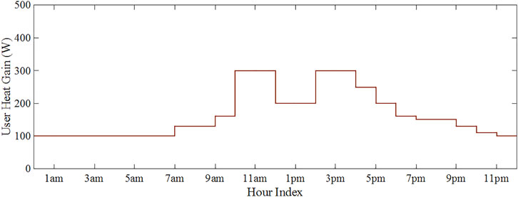
FIGURE 9. Heat gain released by the occupant.
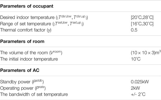
TABLE 1. Settings of major parameters in the home environment.
Six TSAs and two PAAs are simulated for being managed by the HEMS. The configurations of these appliances are given in Table 2, note that the heat gain released by the
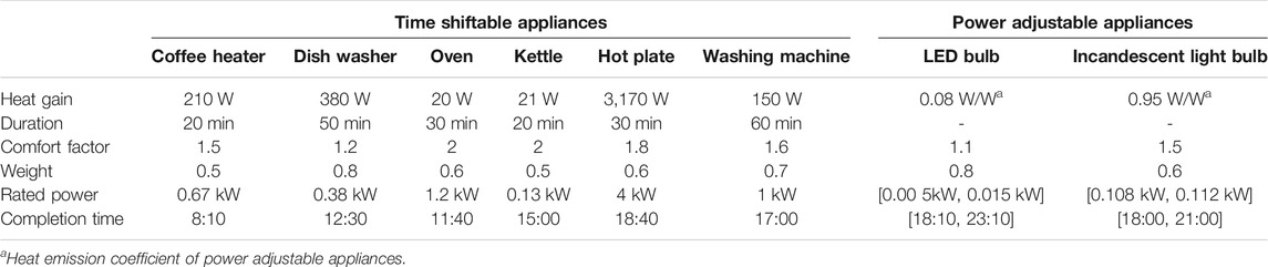
TABLE 2. Settings of controllable appliances.
The home is considered to be charged by a real-time electricity pricing (RTP) scheme, shown as Figure 10. A 24-h scheduling period is considered with the duration of each time slot (
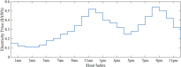
FIGURE 10. Profile of the real-time electricity prices.
Result and Discussion
Following Solving Approach, the MONAA is applied to solve the proposed HEMS. The execution time of the optimization depends on various factors, including the pre-specified maximum generation time and population size, the pre-specified control interval, the number of TSAs, the number and configuration of PAAs, and the hardware configuration of the processor that executes the optimization. With the simulation settings reported in this paper, a total of 15 min is spent on performing the optimization, which is acceptable for an ex-ante appliance scheduling task. The Pareto Frontier consisting of 112 non-dominated solutions is obtained, where each solution represents a home energy management scheme. Figure 11 shows these non-dominated solutions as well as their projections on each 2-objective space.
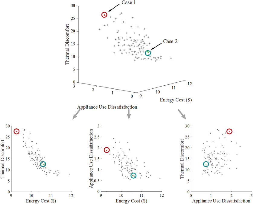
FIGURE 11. Obtained non-dominated home energy management solutions.
Figure 11 generally shows that the proposed HEMS effectively generates diverse solutions to achieve different compromises among the three energy management objectives. To demonstrate the home energy management effect with more detail, we select two specific cases from the generated Pareto Frontier and compare the two cases with another benchmark case:
1) Case 1—the home energy management solution with lowest energy cost, denoted by the red spot in Figure 11.
2) Case 2—the home energy management solution chosen from the Pareto Frontier using the compromise-solution method (Solving Approach), denoted by the green spot in Figure 11.
3) Case 3—the benchmark case without energy management. That is, each TSA completes its task at the desired time slot; each PAA operates at the desired power level; the AC operates in a natural heating cycling mode: when the indoor temperature achieves
Table 3 shows the objective values under the three cases. It can be seen that the home energy management solution in Case 1 can produce approximately $1.30 and $4.50 cost savings comparing with Cases 2 and 3 at the expense of a higher dissatisfaction level to the occupant. For the case without energy management (Case 3), it produces little dissatisfaction to the occupant, but also leads to a very large energy cost ($13.87). Figure 12 shows the corresponding profiles of the home’s total power consumption under the three cases. Obviously, in the case without energy management measures (Cases 3), more energy is consumed in the peak (at noontime) and moderate electricity price hours. In Cases 2 and 3, not only are the power consumptions in these hours less than Case 3, but the total energy consumption over the day is also reduced. This is mainly because of the reduced AC operation in Cases 1 and 2, as further discussed in the rest of this section.
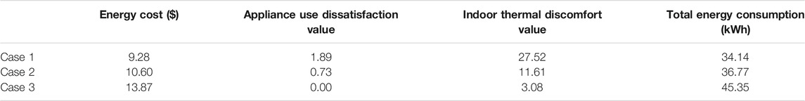
TABLE 3. Objective values under three cases.
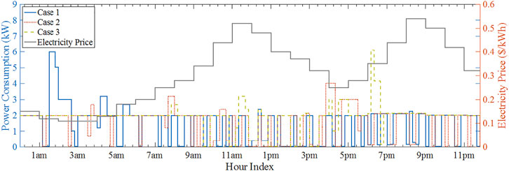
FIGURE 12. Total power consumption profiles under the three cases.
Figure 13 visualizes the schedule for TSAs with and without energy management. The arrows in the figure denote shifting of the appliances’ operation time from the occupant’s desired completion time to the optimized completion time. The optimized results of the LED bulb and incandescent light bulb under Case 1 and Case 2 are shown in Figure 14A,B, respectively, where the green block represents the power range of the LED bulb. While in Case 3, the power of the LED bulb is 0.015 kW and the power of the incandescent light bulb is 0.112 kW. Detailed appliance use discomfort values of these controllable appliances (calculated following Modelling of Occupant’s Dwelling Satisfaction) are listed in Table 4.
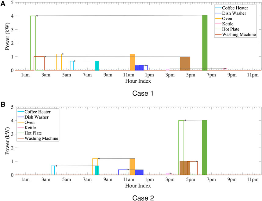
FIGURE 13. Planned schedule of TSAs under Case 1 and Case 2 (lines: optimized completion time of each TSA by MONAA; blocks: user-specified completion time of each TSA).
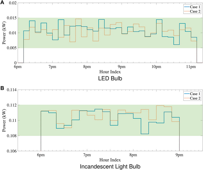
FIGURE 14. Power consumptions of the PAAs under two cases.
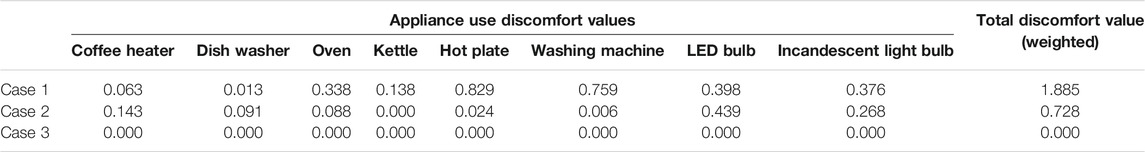
TABLE 4. Appliance use dissatisfaction values.
It can be seen that the optimized completion time of TSAs and the power consumptions of PAAs are different with the ones originally desired by the occupant, due to the consideration of reducing the home energy cost. Particularly, in Case 1 that produces the least home energy cost, it can be seen that a majority of the TSAs (e.g., washing machine and hot plate) are scheduled to operate at midnight, and this also yields significant dwelling dissatisfaction to the occupant. In contrast, the appliance schedules in Case 2 produce a larger energy cost but a lower dissatisfaction level than Case 1.
Figure 15 shows the resulted indoor thermal environments under the three cases. It can be seen that in the natural heating cycling mode (Case 3), the AC keeps running almost the whole late evening and midnight time due to the low outdoor air temperature; as a result, the indoor temperature is kept around 24 Celsius to maintain the maximum thermal comfort level to the occupant. Without performing energy management when subjected to the time-varying electricity tariff, the energy cost due to the AC’s operation is $12.19. For Cases 1 and 2, compared with Case 3, the AC’s operation time is reduced in the peak electricity price hours (i.e., 11 am-1 pm and 8–10 pm), leading to a lower energy cost for AC operation ($8.46 in Case 1 and $9.28 in Case 2, respectively). For the exchange of the reduced energy cost, the indoor temperature under Cases 1 and 2 deviate from the comfort temperature range more frequently, leading to a lower thermal comfort degree for the occupant.
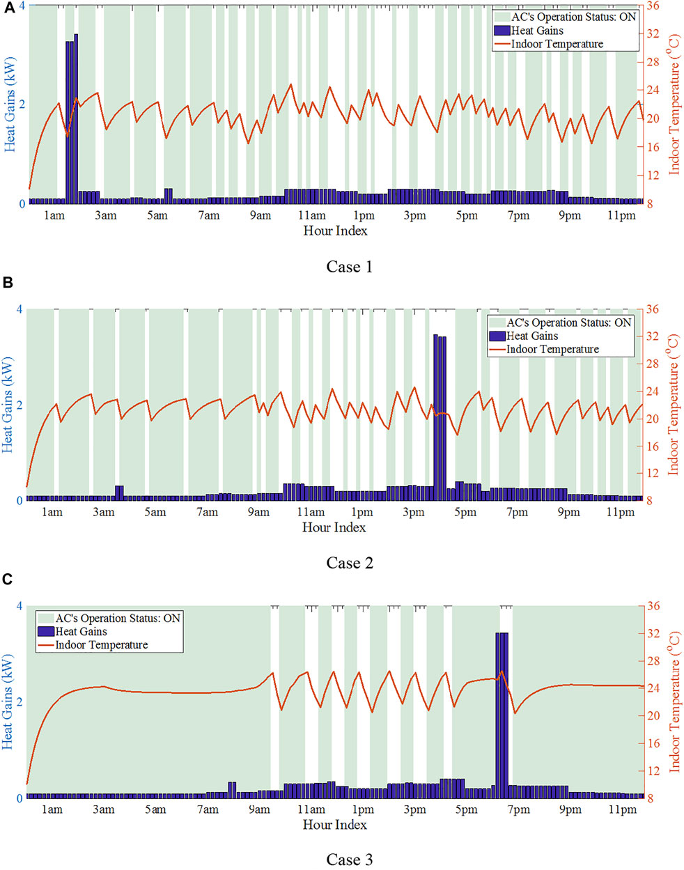
FIGURE 15. Indoor thermal environment and AC operation status.
Figure 15 also shows that the internal heat gain distribution of the room has an impact on the AC’s operation. Taking Case 3 as an example, when there is high internal heat gain released by the appliances and the occupant (around 6–7 pm, mainly because of the operation of the hot plate), the room is warmed, meaning the AC can be turned off temporarily even though the outdoor temperature at that time is low. A similar phenomenon is also observed in Cases 1 and 2. Such an impact indicates that heat gain-aware coordinated scheduling of AC and other appliances would be meaningful for optimizing the energy performance of a home, which is less investigated in the existing literature.
Conclusion and Future Work
This paper studies the home energy management problem when subjected to a real-time electricity price environment. Flexible satisfaction and comfort models are established, which use adjustable parameters to reflect individual occupants’ appliance usage and thermal comfort preferences. Based on these models, a new multi-objective home energy management model is established. Numerical simulations demonstrate that when comparing the existing literature, the proposed system can model the home energy management process in a more realistic manner in terms of balancing the different considerations in a home environment and accounting for the impact of the room’s internal heat gain on the AC’s operation.
The HEMS proposed in this paper is expected to enhance automation and energy efficiency in the residential sector. Future work can be conducted in two directions. Firstly, the authors are planning a user survey and field testing to collect data to fit the parameters in the theoretical satisfaction models proposed in this paper. Secondly, the HEMS proposed in this paper can be expanded to integrate renewable energy sources and energy storage systems. More sophisticated thermal models can also be integrated into the proposed home energy framework without significant modifications.
Data Availability Statement
The original contributions presented in the study are included in the article/supplementary files, further inquiries can be directed to the corresponding author.
Author Contributions
FL designed experiments; ZZ carried out experiments. YZ analyzed experimental results. YZ approved the final version of the paper for publication. SS made important revisions to the paper. ZZ and FL. wrote the article.
Funding
This research is supported by the National Natural Science Foundation of China (no. 51777015, 51807011).
Conflict of Interest
The authors declare that the research was conducted in the absence of any commercial or financial relationships that could be construed as a potential conflict of interest.
Publisher’s Note
All claims expressed in this article are solely those of the authors and do not necessarily represent those of their affiliated organizations, or those of the publisher, the editors and the reviewers. Any product that may be evaluated in this article, or claim that may be made by its manufacturer, is not guaranteed or endorsed by the publisher.
References
Deng, Y., Zhang, Y., Luo, F., and Mu, Y. (2021). Operational Planning of Centralized Charging Stations Utilizing Second-Life Battery Energy Storage Systems. IEEE Trans. Sustain. Energ. 12, 387–399. doi:10.1109/TSTE.2020.3001015
Ding, Y., Song, Y., Hui, H., and Shao, C. (2019). Integration of Air Conditioning and Heating into Modern Power Systems: Enabling Demand Response and Energy Efficiency. Singapore: Springer Singapore. doi:10.1007/978-981-13-6420-4
Dorokhova, M., Ballif, C., and Wyrsch, N. (2020). Rule-based Scheduling of Air Conditioning Using Occupancy Forecasting. Energy and AI 2, 100022. doi:10.1016/j.egyai.2020.100022
Fong, K. F., Hanby, V. I., and Chow, T. T. (2006). HVAC System Optimization for Energy Management by Evolutionary Programming. Energy and Buildings 38, 220–231. doi:10.1016/j.enbuild.2005.05.008
Gupta, S. K., Kar, K., Mishra, S., and Wen, J. T. (2015). Collaborative Energy and thermal comfort Management through Distributed Consensus Algorithms. IEEE Trans. Automat. Sci. Eng. 12, 1285–1296. doi:10.1109/TASE.2015.2468730
Gupta, S. K., Kar, K., Mishra, S., and Wen, J. T. (2018). Incentive-based Mechanism for Truthful Occupant comfort Feedback in Human-In-The-Loop Building thermal Management. IEEE Syst. J. 12, 3725–3736. doi:10.1109/JSYST.2017.2771528
Heat Gain from People, Lights, and Appliances Heat Gain from People, Lights, and Appliances. Available at: https://engineer-educators.com/topic/5-heat-gain-from-people-lights-and-appliances/. (Accessed May 31, 2020).
Hornyak, T. (2011). Nissan Smart Home Powered by Leaf Battery. Available at: https://www.cnet.com/news/nissan-smart-home-powered-by-leaf-battery/. (Accessed May 31, 2021).
Inoue, M., Higuma, T., Ito, Y., Kushiro, N., and Kubota, H. (2003). Network Architecture for home Energy Management System. IEEE Trans. Consumer Electron. 49, 606–613. doi:10.1109/TCE.2003.1233782
Iwafune, Y., Ikegami, T., Fonseca, J. G. d. S., Oozeki, T., and Ogimoto, K. (2015). Cooperative home Energy Management Using Batteries for a Photovoltaic System Considering the Diversity of Households. Energ. Convers. Manag. 96, 322–329. doi:10.1016/j.enconman.2015.02.083
Jindal, A., Bhambhu, B. S., Singh, M., Kumar, N., and Naik, K. (2020). A Heuristic-Based Appliance Scheduling Scheme for Smart Homes. IEEE Trans. Ind. Inf. 16, 3242–3255. doi:10.1109/TII.2019.2912816
Jo, H.-C., Kim, S., and Joo, S.-K. (2013). Smart Heating and Air Conditioning Scheduling Method Incorporating Customer Convenience for home Energy Management System. IEEE Trans. Consumer Electron. 59, 316–322. doi:10.1109/TCE.2013.6531112
Liu, C., Chau, K. T., Wu, D., and Gao, S. (2013). Opportunities and Challenges of Vehicle-to-Home, Vehicle-To-Vehicle, and Vehicle-To-Grid Technologies. Proc. IEEE 101, 2409–2427. doi:10.1109/JPROC.2013.2271951
Luo, F. J., Ranzi, G., Dong, Z. Y., and Murata, J. (2017a). “Natural Aggregation Approach Based Home Energy Manage System with User Satisfaction Modelling,” in International Conference on Sustainable Energy Engineering, 12–14 June 2017 (Perth, Australia), 012005. doi:10.1088/1755-1315/73/1/012005
Luo, F., Ranzi, G., Kong, W., Dong, Z. Y., and Wang, F. (2018). Coordinated Residential Energy Resource Scheduling with Vehicle‐to‐home and High Photovoltaic Penetrations. IET Renew. Power Generation 12, 625–632. doi:10.1049/iet-rpg.2017.0485
Luo, F., Ranzi, G., Liang, G., and Dong, Z. Y. (2017b). “Stochastic Residential Energy Resource Scheduling by Multi-Objective Natural Aggregation Algorithm,” in 2017 IEEE Power & Energy Society General Meeting, Chicago, IL, 16-20 July 2017 (IEEE), 1–5. doi:10.1109/PESGM.2017.8274308
Luo, F., Ranzi, G., Wan, C., Xu, Z., and Dong, Z. Y. (2019). A Multistage Home Energy Management System with Residential Photovoltaic Penetration. IEEE Trans. Ind. Inf. 15, 116–126. doi:10.1109/TII.2018.2871159
Luo, F., Zhao, J., and Dong, Z. Y. (2016). “A New Metaheuristic Algorithm for Real-Parameter Optimization: Natural Aggregation Algorithm,” in 2016 IEEE Congress on Evolutionary Computation (CEC), Vancouver, BC, Canada, 24-29 July 2016 (IEEE), 94–103. doi:10.1109/CEC.2016.7743783
Marler, R. T., and Arora, J. S. (2004). Survey of Multi-Objective Optimization Methods for Engineering. Struct. Multidisciplinary Optimization 26, 369–395. doi:10.1007/s00158-003-0368-6
Mathieu, J. L., Price, P. N., Kiliccote, S., and Piette, M. A. (2011). Quantifying Changes in Building Electricity Use, with Application to Demand Response. IEEE Trans. Smart Grid 2, 507–518. doi:10.1109/TSG.2011.2145010
Ozturk, Y., Senthilkumar, D., Kumar, S., and Lee, G. (2013). An Intelligent Home Energy Management System to Improve Demand Response. IEEE Trans. Smart Grid 4, 694–701. doi:10.1109/tsg.2012.2235088
Rastegar, M., Fotuhi-Firuzabad, M., and Aminifar, F. (2012). Load Commitment in a Smart home. Appl. Energ. 96, 45–54. doi:10.1016/j.apenergy.2012.01.056
Ryder-Cook, D. (2009). Thermal Modelling of Buildings. Cambridge, United Kingdom: Cavendish Laboratory, Department of Physics. University of Cambridge.
Suszanowicz, D. (2017). Internal Heat Gain from Different Light Sources in the Building Lighting Systems. E3s Web Conf. 19, 01024. doi:10.1051/e3sconf/20171901024
Zhang, Y., Xu, Y., Yang, H., Dong, Z. Y., and Zhang, R. (2020). Optimal Whole-Life-Cycle Planning of Battery Energy Storage for Multi-Functional Services in Power Systems. IEEE Trans. Sustain. Energ. 11, 2077–2086. doi:10.1109/TSTE.2019.2942066
Zhuang Zhao, Z., Won Cheol Lee, W. C., Yoan Shin, Y., and Kyung-Bin Song, K.-B. (2013). An Optimal Power Scheduling Method for Demand Response in Home Energy Management System. IEEE Trans. Smart Grid 4, 1391–1400. doi:10.1109/TSG.2013.2251018
Nomenclature
Parameters
Variables
Keywords: demand response, smart home, building energy, smart grid, demand side management
Citation: Zhao Z, Luo F, Zhang Y, Ranzi G and Su S (2021) Integrated Household Appliance Scheduling With Modeling of Occupant Satisfaction and Appliance Heat Gain. Front. Energy Res. 9:724189. doi: 10.3389/fenrg.2021.724189
Received: 12 June 2021; Accepted: 04 August 2021;
Published: 13 September 2021.
Edited by:
Yang Li, Northeast Electric Power University, ChinaReviewed by:
Santosh Gupta, Santa Clara University, United StatesJagriti Saini, National Institute of Technical Teachers Training and Research, India
Rongxing Hu, North Carolina State University, United States
Copyright © 2021 Zhao, Luo, Zhang, Ranzi and Su. This is an open-access article distributed under the terms of the Creative Commons Attribution License (CC BY). The use, distribution or reproduction in other forums is permitted, provided the original author(s) and the copyright owner(s) are credited and that the original publication in this journal is cited, in accordance with accepted academic practice. No use, distribution or reproduction is permitted which does not comply with these terms.
*Correspondence: Yongxi Zhang, aXNzdWtpMzMwQDEyNi5jb20=