AutoMoG 3D: Automated Data-Driven Model Generation of Multi-Energy Systems Using Hinging Hyperplanes

The optimal operation of multi-energy systems requires optimization models that are accurate and computationally efficient. In practice, models are mostly generated manually. However, manual model generation is time-consuming, and model quality depends on the expertise of the modeler. Thus, reliable and automated model generation is highly desirable. Automated data-driven model generation seems promising due to the increasing availability of measurement data from cheap sensors and data storage. Here, we propose the method AutoMoG 3D (Automated Model Generation) to decrease the effort for data-driven generation of computationally efficient models while retaining high model quality. AutoMoG 3D automatically yields Mixed-Integer Linear Programming models of multi-energy systems enabling efficient operational optimization to global optimality using established solvers. For each component, AutoMoG 3D performs a piecewise-affine regression using hinging-hyperplane trees. Thereby, components can be modeled with an arbitrary number of independent variables. AutoMoG 3D iteratively increases the number of affine regions. Thereby, AutoMoG 3D balances the errors caused by each component in the overall model of the multi-energy system. AutoMoG 3D is applied to model a real-world pump system. Here, AutoMoG 3D drastically decreases the effort for data-driven model generation and provides an accurate and computationally efficient optimization model.

1 Introduction

Multi-energy systems are regarded as key element of future sustainable energy systems since they can efficiently integrate the conversion of several energy inputs and outputs (Mancarella et al., 2016; Guelpa et al., 2019; Moretti et al., 2020). For this purpose, multi-energy systems usually consist of many components. Due to the resulting complexity, the optimal design and operation of multi-energy systems are best addressed by optimization models (Mancarella, 2014; Andiappan, 2017; Thie et al., 2020). Optimization models represent the input-output relationship of each component to capture its operation. For practical use, the optimization model has to be sufficiently accurate (Welsch et al., 2014).

For operational optimization, the model will usually be solved repeatedly to reflect changes in demands, resource availability, or prices (Wang et al., 2015). Thus, the model has to be not only sufficiently accurate but also computationally efficient.

Accuracy and computational efficiency of the multi-energy system model result from model generation. Today, models of multi-energy systems are commonly generated manually. To model multi-energy systems, measured data can often be used. Measured data is increasingly available for multi-energy systems, e.g., due to the implementation of energy management systems according to ISO 50001:2018 (2018). Still, model generation requires high effort and, therefore, is time-consuming (Bonvin et al., 2016).

To decrease the effort for model generation, methods for automated data-driven modeling have been proposed. Cozad et al. (2014) and Wilson and Sahinidis (2017) developed ALAMO for Automated Learning of Algebraic MOdels. ALAMO derives algebraic models from measured data or simulations. For an overview of data-driven modeling, the reader is referred to McBride and Sundmacher (2019).

However, the data-driven models are in general nonlinear. Thus, the subsequent optimization problem is usually a Mixed-Integer Nonlinear Program (MINLP). In practice, MINLPs are still challenging to solve to global optimality (Mitsos et al., 2018). Thus, for multi-energy systems, nonlinear input-output relationships of components are often approximated by piecewise-affine models leading to Mixed-Integer Linear Programs (MILPs) (Voll et al., 2013; Zhang et al., 2016). Optimization problems of multi-energy systems are often formulated as MILPs because MILPs enable finding the global optimum with established solvers (Kantor et al., 2020).

The efficient generation of accurate and computationally efficient piecewise-affine models yields in general complex MINLPs itself and is therefore an active field of research. Recently, Kong and Maravelias (2020) and Rebennack and Krasko (2020) formulate MILP approaches for continuous piecewise-affine regression. These MILP approaches derive univariate continuous piecewise-affine models from measured data. While these approaches overcome the MINLP problem, they do not reflect the complex structure of multi-energy systems. For this purpose, some of the present authors proposed the AutoMoG method to provide MILP optimization models of multi-energy systems from measured data (Kämper et al., 2021). AutoMoG also represents the components of the multi-energy system by univariate continuous piecewise-affine models. In contrast to common practice, AutoMoG does not model each component independently, which may lead to an unnecessarily complicated model of the overall multi-energy system. Instead, AutoMoG balances the errors caused by the model of each component in the overall multi-energy system model.

However, the described approaches are restricted to multi-energy systems that contain components with one independent variable, e.g., the heat output of a boiler solely depends on its fuel input. In general, the input-output relationship of a component depends on multiple independent variables, e.g., the power consumption of a pump depends on its rotational speed and volumetric flow rate. Another typical component in energy systems is a combined-heat-and-power (CHP) plant. The heat output of a CHP plant that consists of a gas turbine and post-firing depends on the heat output of the gas turbine and the gas input of the post-firing (Bischi et al., 2014). Deriving these input-output relationships from measured data leads to multidimensional piecewise-affine regression problems.

Various approaches generate multidimensional piecewise-affine models that are suitable for MILP optimization. Fischetti and Jo (2018) and Grimstad and Andersson (2019) showed that deep neural networks with rectified linear units as activation functions can be formulated as MILP models. Thus, the deep neural networks can approximate a nonlinear model with arbitrary accuracy and then be embedded in a subsequent MILP optimization (Katz et al., 2020). However, efficiently embedding deep neural networks in MILPs is challenging, and thus, an active field of research (Anderson et al., 2020).

Recently, Obermeier et al. (2021) proposed two approaches to generate multidimensional piecewise-affine models from measured data. Both approaches create a mesh using all data points with Delauney triangulation (Barber et al., 1996). The first approach IMRed (Iterative Mesh Reduction) iteratively reduces the complexity of the created mesh by contracting the edges of this mesh. The second approach IMRef (Iterative Mesh Refinement) chooses one affine region of the created mesh to represent all data points. Then, IMRef iteratively increases the affine regions to represent all data points until a predefined accuracy is reached. Furthermore, Kazda and Li (2021) proposed a method for multidimensional piecewise-affine fitting using the difference-of-convex representation. The method aims to generate a model with predefined accuracy while keeping the number of affine regions low. The approaches of Obermeier et al. (2021) and Kazda and Li (2021) are designed to transform a well-defined functional relationship or handle noiseless data and not to handle noisy measured data obtained in real-world applications.

However, hinging hyperplanes (Breiman, 1993) have been shown to handle well-defined functional relationships as well as noisy measured data (Roll et al., 2004). Hinging-hyperplane-tree regression (Ernst, 1998) is based on the hinge-finding algorithm (Breiman, 1993) and can solve multidimensional piecewise-affine regression problems. However, the original hinge-finding algorithm (Breiman, 1993) suffers from convergence problems. To overcome this drawback, an improved hinge-finding algorithm has been developed (Pucar and Sjöberg, 1998). Roll et al. (2004) used hinging hyperplanes in an MILP approach to solve multidimensional piecewise-affine regression problems at the price of increased computational effort.

Here, we combine the hinging-hyperplane-tree regression (Ernst, 1998) with the improved hinge-finding algorithm (Pucar and Sjöberg, 1998). The hinging-hyperplane trees offer easy control of the resulting complexity of the data-driven models. However, in general, the resulting models show discontinuities between the hyperplanes. Still, we find that the hinging-hyperplane trees are able to generate efficient and accurate models for MILP optimization. In result, hinging-hyperplane trees seem promising for multi-energy system modeling.

Thus, in this work, we propose the method AutoMoG 3D to generate automatically MILP optimization models of multi-energy systems that contain components with multiple independent variables. The input-output relationship of the components is derived from the measured data of the components. AutoMoG 3D uses the improved hinge-finding algorithm of Pucar and Sjöberg (1998) in the hinging-hyperplane tree approach of Ernst (1998) to solve the multidimensional piecewise-affine regression problems. In general, other methods to solve the multidimensional piecewise-affine regression problems can easily be used in AutoMoG 3D. AutoMoG 3D builds on the advantages of the AutoMoG method (Kämper et al., 2021), i.e., AutoMoG 3D considers the importance of the components in context of the overall multi-energy system. The models generated by AutoMoG 3D are suitable for MILP optimization. AutoMoG 3D is particularly useful to generate efficient MILP optimization models from measured data, and thus, for operational optimization. However, AutoMoG 3D is not limited to generate models for operational optimization from measured data but can also generate models for synthesis problems, as shown in the case study.

The remainder of the paper is organized as follows: In Section 2, we describe the general workflow of AutoMoG 3D and discuss in detail the use of hinging-hyperplane trees. In Section 3, we apply AutoMoG 3D to model an industrial real-world pump system. In Section 4, we conclude with the key findings.

2 AutoMoG 3D Method for Model Generation

AutoMoG 3D aims at modeling multi-energy systems that contain components with multiple independent variables. AutoMoG 3D uses measured data to obtain piecewise-affine models of components. Due to the multiple independent variables, AutoMoG 3D has to solve multidimensional piecewise-affine regression problems. The multidimensional piecewise-affine regression problems are solved using hinging-hyperplane trees (Ernst, 1998). We describe the general workflow of AutoMoG 3D in Section 2.1 and the use of hinging-hyperplane trees in AutoMoG 3D in Section 2.2.

2.1 General Workflow of AutoMoG 3D

The original AutoMoG method (Kämper et al., 2021) is limited to multi-energy systems that contain components with one independent variable. A component is a physical unit or a subsection of the multi-energy system. Here, we extend AutoMoG to AutoMoG 3D, enabling the modeling of multi-energy systems that contain components with multiple independent variables.

The general workflow of AutoMoG 3D is illustrated in Figure 1. As a starting point, AutoMoG 3D needs the measured input and output data of each component. AutoMoG 3D derives the component models from these measured input and output data. Thus, the component models derived by AutoMoG 3D can only be as accurate as the measured data reflect the actual component behavior.

FIGURE 1

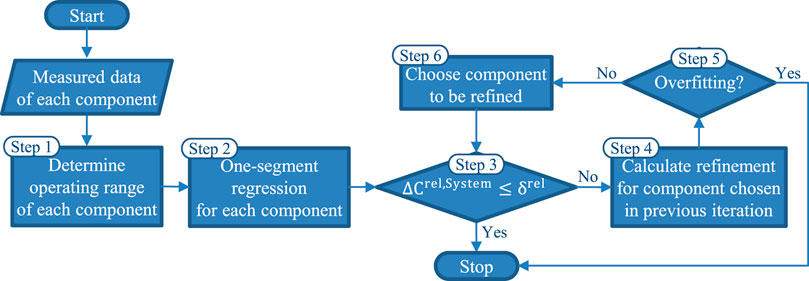
FIGURE 1. AutoMoG 3D for multidimensional automated model generation using hinging-hyperplane trees. ΔC^rel,System is the relative error of the overall multi-energy system model. δ^rel is the allowed relative error of the overall multi-energy system model as specified by the user.

In step 1, AutoMoG 3D determines the operating range of each component. The operating range of a component describes the feasible region of its model in a subsequent optimization. To determine the operating range of a component, AutoMoG 3D calculates the convex hull (Barber et al., 1996) around the input data of the component. For this reason, the components’ input data should ideally reflect its entire operating range. The edges of all convex hulls are then added to the subsequent optimization problem as inequality constraints that limit the feasible region of the components’ models.

In step 2, AutoMoG 3D initializes the multi-energy system model by performing a linear regression with one region (one segment) for each component minimizing the mean squared error.

In step 3, AutoMoG 3D checks the accuracy of the overall multi-energy system model. For this purpose, the AutoMoG approach introduced by Kämper et al. (2021) is followed. The errors between model and measured data of all components are aggregated to the relative error of the overall multi-energy system ΔC^rel,System. For this purpose, the errors of all components are weighted by weighting factors that reflect the components’ model errors in terms of cost. The user can specify a weighting factor for each component’s dependent variable in the multi-energy system. If the multi-energy system is modeled for economic optimization, cost-based weighting factors for the dependent variables are appropriate. Typically, the dependent variable of a component is an energy form (e.g., power consumption, gas input, etc.), and the cost-based weighting factor can be derived from the cost of this energy form (Kämper et al., 2021). By using cost-based weighting factors, AutoMoG 3D takes into account that components with high energy costs are more important for the operation of the actual multi-energy system. However, other weighting factors can be used easily, e.g., primary energy factors or CO₂-eq. if the model is used for environmental optimization.

AutoMoG 3D terminates if the relative error of the overall multi-energy system ΔC^rel,System reaches the allowed relative error of the overall multi-energy system δ^rel. The allowed relative error of the overall multi-energy system δ^rel is specified by the user. If the allowed relative error of the overall multi-energy system δ^rel is not reached, AutoMoG 3D proceeds with step 4.

Instead of this accuracy check, it is also possible to limit the model complexity by specifying the number of piecewise-affine regions in the multi-energy system model. In this case, AutoMoG 3D terminates if the pre-specified number of piecewise-affine regions is reached. Alternatively, the iterative process of AutoMoG 3D and the computational efficiency of the hinging-hyperplane trees allow considering the actual operational optimization during model generation. Thereby, the objective function of the operational optimization could decide which component to refine and when to terminate AutoMoG 3D. This approach will be explored in future work.

In step 4, AutoMoG 3D uses hinging-hyperplane trees to calculate the next possible refinement (Section 2.2) for the component that was refined in the previous iteration. In the first iteration, AutoMoG 3D calculates the next refinement for all components in the multi-energy system. In result, the next possible refinement of each component is always known. Based on the next possible refinement of each component, AutoMoG 3D chooses one component to be refined in step 6.

However, before choosing one component to be refined, in step 5, AutoMoG 3D checks if overfitting might appear in the component models. For this purpose, AutoMoG 3D employs the Corrected Akaike Information Criterion AIC_C (Hurvich and Tsai, 1993) to the next possible refinement of each component. The Corrected Akaike Information Criterion AIC_C (Hurvich and Tsai, 1993) is an extension of the Akaike Information Criterion AIC (Akaike, 1974) suitable for small sample sizes. However, any information criterion can be used in AutoMoG 3D, e.g., the widely known Bayesian Information Criterion BIC (Stoica and Selén, 2004). AutoMoG 3D does not refine any component for which the chosen information criterion (here: AIC_c) indicates overfitting. Thus, AutoMoG 3D terminates if the chosen information criterion indicates overfitting for every component. Otherwise, AutoMoG 3D proceeds with step 6.

In step 6, AutoMoG 3D chooses a component to be refined based on the expected improvement in the overall error of the multi-energy system model. Based on the calculated next refinements of all components, AutoMoG 3D checks the improvement in the overall error of the multi-energy system model. The component with the greatest improvement in the overall error is chosen to be refined. By default, AutoMoG 3D uses the sum of squared residuals as error measure. Thereby, components with many data points tend to have a higher component model error, and thus, are more likely chosen to be refined. Thus, the sum of squared residuals is a meaningful error measure if the number of data points reflects the importance of a component. However, if the number of data points does not reflect the importance of a component, alternative error measures could be used, e.g., the mean squared error where the sum of squared residuals is divided by the number of data points for each component. After step 6, AutoMoG 3D continues with step 3.

By the iteration of steps 3 to 6, AutoMoG 3D increases the accuracy of the overall multi-energy system model until either the given accuracy is reached or all components in the multi-energy system would be overfitted when further refined.

Thereby, AutoMoG 3D allows for efficient modeling as the component models are evaluated in context to the overall multi-energy system. More details on these steps can be found in Kämper et al. (2021). In the following, we present the details of the hinging-hyperplane trees, which is the main innovation of AutoMoG 3D compared to the original AutoMoG method.

2.2 Multidimensional Piecewise-Affine Regression Using Hinging-Hyperplane Trees

In step 4, AutoMoG 3D uses the hinging-hyperplane trees to solve the multidimensional piecewise-affine regressions for the components of a multi-energy system. Hinging-hyperplane trees are based on the hinging-hyperplane method (Breiman, 1993). The hinging-hyperplanes method generates a hinge function that can be used for regression, classification, and function approximation. The hinge function consists of two hyperplanes and their intersection, the hinge (Figure 2). The resulting hinge function h is continuous. The two hyperplanes h⁺ and h⁻ are described by

$h^{+}={\mathbf{x}}^T{\mathit{\theta }}^{+},h^{-}={\mathbf{x}}^T{\mathit{\theta }}^{-},(1)$

where $\mathbf{x}={[1,x_1,x_2\dots ..x_M]}^T$ are the independent variables in M dimensions, and θ⁺ and θ⁻ are the parameters of the hyperplanes. The hinge Δ = θ⁺ −θ⁻ is the joint of the hyperplanes and fulfills

${\mathbf{x}}^T\mathbf{\Delta }=0.(2)$

FIGURE 2

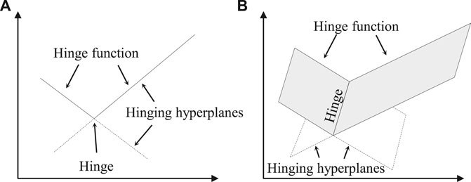
FIGURE 2. Sketch of hinging hyperplanes, the hinge, and the hinge function are illustrated in two dimensions (A) and three dimensions (B), adapted from Pucar and Sjöberg (1998).

The hinge function h is either the minimum or the maximum of the two hyperplanes, depending on the fitting task (cf. Figure 2):

$h=\text{min}(\text{or}\text{max})\left\{h^{+},h^{-}\right\}.(3)$

Breiman (1993) proposed the hinge-finding algorithm that efficiently determines a good position for the hinge to approximate measured data or a function with two hyperplanes. The hinge-finding algorithm assigns each data point to one hyperplane and, thus, separates the measured data into two data subsets. Ernst (1998) combined the hinge-finding algorithm of Breiman (1993) with binary-tree regression, leading to hinging-hyperplane trees. A hinging-hyperplane tree starts with applying the hinge-finding algorithm to the measured data to be approximated. After the hinge-finding algorithm separated the measured data into two data subsets and fitted each data subset with one hyperplane, the worse of the two fitted data subsets is identified. Subsequently, the worst fitted data subset is further refined by applying the hinge-finding algorithm again. By iteratively applying the hinge-finding algorithm, hinging-hyperplane trees can approximate measured data with an arbitrary number of hyperplanes. Ernst (1998) used hinging-hyperplane trees for efficient approximation of nonlinear functions. However, in each iteration, the hinge-finding algorithm only separates the data points of the worst fitted data subset. Thus, in general, hinging-hyperplane trees generate a non-continuous piecewise-affine function.

Hinging-hyperplane trees enable axis-oblique partitioning of measured data. This axis-oblique partitioning allows a more flexible fit to the measured data than axis-orthogonal partitioning, which is used in common tree-based regression (Ernst, 1998).

However, the hinge-finding algorithm of Breiman (1993) used in Ernst (1998) suffers from convergence problems (Kenesei and Abonyi, 2015). To solve the convergence problems of the hinge-finding algorithm, Pucar and Sjöberg (1998) showed that the hinge-finding algorithm is equivalent to a Newton algorithm that minimizes the squared residuals between measured data and the hinge function. Pucar and Sjöberg (1998) introduced a damping parameter, following the idea of a damped Newton algorithm, and thereby extended the convergence range of the hinge-finding algorithm. In AutoMoG 3D, we use the improved hinge-finding algorithm (Pucar and Sjöberg, 1998) to calculate hinging-hyperplane trees. The input of the improved hinge-finding algorithm is a data set. The improved hinge-finding algorithm performs a least-squares regression with the fitting criterion V_N that is defined by

$V_N=\frac{1}{2}\sum _{n=\mathrm{1}}^N{(y_n-h({\mathit{x}}_{\mathit{n}},\mathit{\theta }))}^2.(4)$

N is the number of data points in the given data set, y_n and x_n are the values in data point n from the given data set, and h (x_n, θ) is the value of the hinge function in data point n. The parameter vector θ contains the parameters for both hyperplanes:

$\mathit{\theta }={\left({\mathit{\theta }}^{+},{\mathit{\theta }}^{-}\right)}^T.(5)$

Thus, the algorithm simultaneously determines the two hyperplanes and thereby the hinge [cf. Eq. (2)]. The improved hinge-finding algorithm applies a damped Newton algorithm to determine the parameter vector θ:

$\hat{\mathit{\theta }}=\underset{\mathit{\theta }}{\mathrm{arg\; min}}{V}_N.(6)$

More details to the improved hinge-finding algorithm can be found in Pucar and Sjöberg (1998).

In step 4, AutoMoG 3D uses the hinging-hyperplane trees to add one piecewise-affine region to the model of a component (Figure 3). One piecewise-affine region corresponds to one hyperplane.

FIGURE 3

FIGURE 3. Flowchart of step 4 in AutoMoG 3D. The worst fitted data subset D is partitioned into two new data subsets D⁺ and D⁻ by the hinge-finding algorithm. The data subsets D⁺ and D⁻ are approximated by the hyperplanes $h_D^{+}$ and $h_D^{-}$, respectively. The hyperplanes $h_D^{+}$ and $h_D^{-}$ are separated at the hinge Δ_D.

In the following, we exemplify step 4 with an arbitrary component that has been chosen to be refined in step 6 of the previous iteration. The component is already modeled by two piecewise-affine regions (cf. Figure 4A). AutoMoG 3D compares the mean squared error in each region of the chosen component. In the given example, the two regions with data subsets $D_1^{+}$ and $D_1^{-}$ exist because the component is modeled by two piecewise-affine regions before applying step 4. The data subset with the highest mean squared error is identified as the worst-fitted data subset D. In this example, the worst-fitted data subset D is $D_1^{-}$. $D_1^{-}$ is refined by the hinge-finding algorithm proposed by Pucar and Sjöberg (1998). The hinge-finding algorithm determines the position of the hinge ${\mathrm{\Delta }}_{{\text{D}}_2}$ that partitions the data subset $D_1^{-}$ into the two new data subsets $D_2^{+}$ and $D_2^{-}$ (Figure 4B).

FIGURE 4

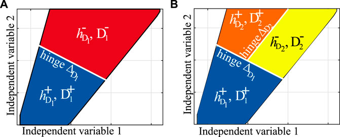
FIGURE 4. Example of step 6 in AutoMoG 3D for an arbitrary component with two independent variables. On the left (A) the measured data are approximated by two hyperplanes. The hyperplane $h_{{\text{D}}_1}^{+}$ approximates the data subset $D_1^{+}$ and the hyperplane $h_{{\text{D}}_1}^{-}$ approximates the data subset $D_1^{-}$. $D_1^{-}$ is the worst-fitted data subset. Thus, on the right (B), the hyperplane $h_{{\text{D}}_1}^{-}$ is partitioned by a new hinge ${\mathrm{\Delta }}_{{\text{D}}_2}$ into two new hyperplanes $h_{{\text{D}}_2}^{+}$ and $h_{{\text{D}}_2}^{-}$ for a better approximation of the measured data.

After the hinge-finding algorithm terminates, the parameters are known for all hyperplanes and hinges of the chosen component. The obtained parameters can directly be used as a component model in an MILP optimization problem.

After step 4, AutoMoG 3D continues with step 5 and checks if the chosen information criterion indicates overfitting for the calculated refinement. When AutoMoG 3D terminates, we obtain an optimization model of the multi-energy system that contains components with multiple independent variables.

3 Case Study: Industrial Real-World Pump System

AutoMoG 3D is applied to model an industrial real-world pump system taken from our previous work (Bahl et al., 2018). We implemented AutoMoG 3D in Matlab and formulated all subsequent optimization problems in GAMS 27.3.0 (GAMS Development Corporation, 2016).

The scheme of the pump system is shown in Figure 5. The purpose of the pump system is to provide cooling water to several customers. The customers differ in their distance to the cooling tower and may have volatile cooling-water demands. Since the customer demand changes for different time steps, the pump system has to provide a wide range of volumetric flow rates and pressure differences. Bahl et al. (2018) and Baumgärtner et al. (2019) solved the synthesis problem for the pump system to reach minimal total annual cost. Thereby, they identified the type and size of each installed pump. At most, six pumps can be installed in the pump system due to limited power supply. Two pump types with three possible sizes each can be installed: three fixed-speed pumps with nominal volumetric flow rates ${\dot{V}}^{\text{nom}}=$ 1,000 m³ h⁻¹, 2000 m³ h⁻¹ and 3,000 m³ h⁻¹, and three variable-speed pumps with the same nominal volumetric flow rates ${\dot{V}}^{\text{nom}}=$ 1,000 m³ h⁻¹, 2000 m³ h⁻¹ and 3,000 m³ h⁻¹, and nominal rotational speed n^nom = 50 Hz. For a fixed-speed pump, the pressure difference and the consumed power are two independent nonlinear functions that depend on its volumetric flow rate $\dot{V}$ only. In contrast, the pressure difference and the consumed power of a variable-speed pump are two independent nonlinear functions that depend on its rotational speed n and volumetric flow rate $\dot{V}$ (Bahl et al., 2018). The nonlinear functions describe the actual behavior of the pumps. In the following, we refer to these nonlinear functions as the actual nonlinear functions of the pumps. The implementation of the actual nonlinear functions leads to an MINLP optimization model. We use this MINLP optimization problem as a benchmark for the AutoMoG 3D model.

FIGURE 5

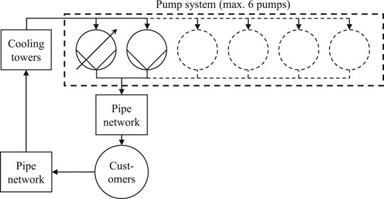
FIGURE 5. Scheme of the industrial real-world pump system (dotted rectangle). The pump system is connected to several customers and cooling towers via a pipe network, adapted from Bahl et al. (2018).

In this case study, we use AutoMoG 3D to generate two MILP models of the pump system. The first AutoMoG 3D model should reach the same model accuracy as the model used by Bahl et al. (2018). For this purpose, we set the desired accuracy δ^rel in step 3 to the accuracy of the MILP model used by Bahl et al. (2018) (cf. Figure 1). The second AutoMoG 3D model can employ the same model complexity as the model used by Bahl et al. (2018). For this purpose, we set the criterion in step 3 to the number of piecewise-affine regions to reach a comparable model resolution as the MILP model used by Bahl et al. (2018). Subsequently, we solve the synthesis problem of the pump-system with the generated AutoMoG 3D models and compare our results to the results from Bahl et al. (2018).

In Section 3.1, we employ AutoMoG 3D. In Section 3.2, we solve the pump-system synthesis problem and analyze the computational efficiency of the AutoMoG 3D model. In Section 3.3, we analyze the solution quality of the AutoMoG 3D model in terms of the total annual cost and the design of the pump system.

3.1 Modeling the Pump System Using AutoMoG 3D

As introduced above, we employ AutoMoG 3D to generate two MILP models of the pump system by linearizing the actual nonlinear functions of the pumps. However, since AutoMoG 3D expects data points as input, we sample the nonlinear functions first. We use 2,500 data points to sample each actual nonlinear function of a variable-speed pump and 50 data points for each actual nonlinear function of a fixed-speed pump.

In the following, we exemplarily illustrate the model generation for the power function of a variable-speed pump in detail. The consumed power of a variable-speed pump depends on its rotational speed n and volumetric flow rate $\dot{V}$, i.e., on two independent variables. The actual nonlinear power function of the variable-speed pump is given by a third-degree polynomial function (Figure 6A).

FIGURE 6

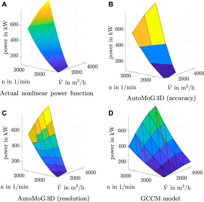
FIGURE 6. Actual nonlinear power function of a variable-speed pump (A), AutoMoG 3D model with the same accuracy as the model of the generalized-convex-combination method (GCCM model) (B), AutoMoG 3D model with a comparable resolution as the GCCM model (C), and the GCCM model used by Bahl et al. (2018)(D). The power depends on the rotational speed n and the volumetric flow rate $\dot{V}$. The generalized-convex-combination method needs a rectangular grid, whereas AutoMoG 3D automatically considers the actual operating limits of the pump. The red lines in (D) show the actual operating limits. The color code only supports the visual differentiation of the piecewise-affine regions.

To obtain an MILP optimization model of the pump system, we apply AutoMoG 3D. For the variable-speed pump, AutoMoG 3D needs four piecewise-affine regions to reach the accuracy of the model used by Bahl et al. (2018) (Figure 6B). We refer to the corresponding model as AutoMoG 3D model (accuracy) in the following. To reach a comparable resolution as the model used by Bahl et al. (2018), AutoMoG 3D needs 18 piecewise-affine regions (Figure 6C). We refer to the corresponding model as AutoMoG 3D model (resolution) in the following. Here, we define comparable resolution by the average area of one piecewise-affine region in the input space.

Bahl et al. (2018) manually linearized the actual nonlinear power function with the generalized-convex-combination method (GCCM) (Geißler, 2011; Geißler et al., 2012) to obtain an MILP optimization model. The generalized-convex-combination method cannot consider the actual operating limits of the power function but needs an axis-orthogonal, rectangular grid. As a result, Bahl et al. (2018) used 40 piecewise-affine regions to model the actual nonlinear power function (Figure 6D). In contrast, AutoMoG 3D automatically considers the actual operating limits for the power function of the variable-speed pump by the convex hull (cf. step 1 in Figure 1).

To compare the model accuracy, we show the relative root squared error of the power function ${ϵ}^{\text{power}}(n,\dot{V})$ over the entire input space (Figure 7). The relative root squared error of the power function ϵ^power is defined as

${ϵ}^{\text{power}}(n,\dot{V})=\frac{\sqrt{{\left(P^{\text{real}}(n,\dot{V})-P^{\text{model}}(n,\dot{V})\right)}^2}}{P^{\text{real}}(n,\dot{V})},(7)$

with the actual power P^real and the modeled power P^model.

FIGURE 7

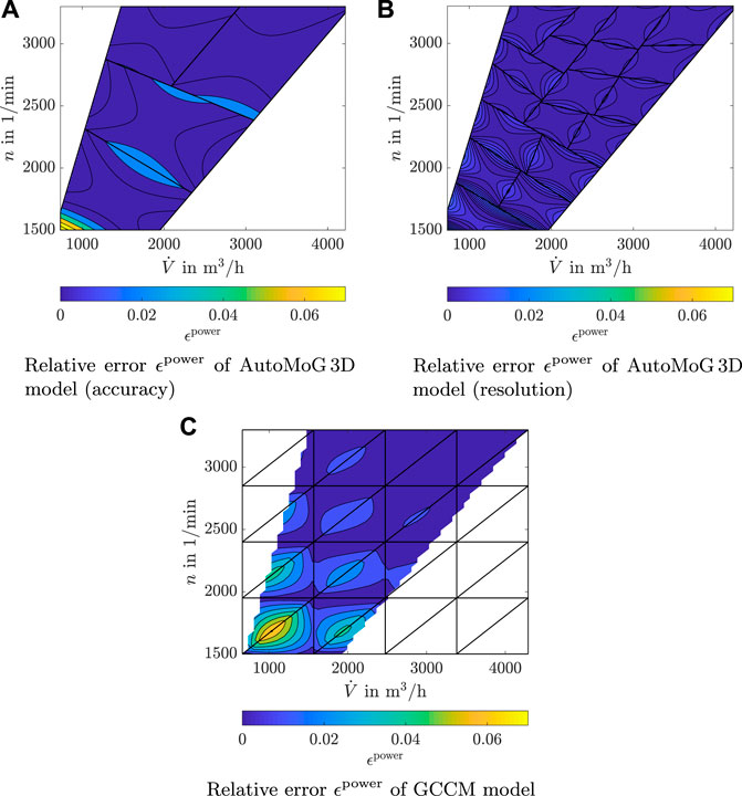
FIGURE 7. Relative error of the AutoMoG 3D model with same accuracy (A) and comparable resolution (B) compared to the relative error of the generalized-convex-combination method (GCCM) model (C) for the power function of a variable-speed pump.

The AutoMoG 3D model (accuracy) and the generalized-convex-combination model show a small relative error ${ϵ}^{\text{power}}(n,\dot{V})$ over a wide operating range (Figures 7A,C). Both models have an average relative error $\overline{{ϵ}^{\text{power}}}$ of 0.01. However, the AutoMoG 3D model (accuracy) uses significantly fewer piecewise-affine regions to approximate the actual nonlinear power function of the variable-speed pump: 4 vs 40. For both models, the relative error ${ϵ}^{\text{power}}(n,\dot{V})$ increases for low rotational speed n and low volumetric flow rate $\dot{V}$ and, in particular, on the edges of the piecewise-affine regions. The error increases for low rotational speed n and low volumetric flow rate $\dot{V}$ because the actual nonlinear function is more curved in this area. Furthermore, the error increases on the edges of the piecewise-affine regions because the hinge-finding algorithm minimizes the mean squared error, and thus tends to a worse fit on the edges.

The AutoMoG 3D model (resolution) has an average relative error $\overline{{ϵ}^{\text{power}}}$ of 0.001 and the generalized-convex-combination model has an average relative error $\overline{{ϵ}^{\text{power}}}$ of 0.01 (Figures 7B,C). However, both models have the same resolution. The AutoMoG 3D model (resolution) reaches a smaller relative error ϵ^power, because AutoMoG 3D refines the regions of the current worst fit. In contrast, the generalized-convex-combination method is based on an inflexible grid.

In summary, compared to the generalized-convex-combination method, AutoMoG 3D can.

1. generate a model with comparable resolution but 10 times higher accuracy.

2. generate a model with 10 times lower resolution but the same accuracy.

For completeness, we briefly show the results of the model generation for the pressure difference of the same variable-speed pump (Figure 8). The pressure head is shown instead of the pressure difference because the pump manufacturer used the head to describe the pressure difference of the variable-speed pump. The head is the height of a liquid column that corresponds to the pressure exerted by this liquid column on its bottom.

FIGURE 8

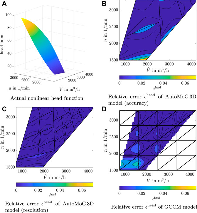
FIGURE 8. Actual nonlinear head function of a variable-speed pump (A), and the relative errors of the AutoMoG 3D model with same accuracy (B) and comparable resolution (C) compared to the relative error of the generalized-convex-combination method (GCCM) model (D) for the head function of a variable-speed pump.

The AutoMoG 3D model (accuracy) and the generalized-convex-combination model have an average relative error $\overline{{ϵ}^{\text{head}}}$ of 0.007 (Figures 8B,D). However, the AutoMoG 3D model (accuracy) again uses only four piecewise-affine regions to approximate the actual nonlinear head function of the variable-speed pump. The generalized-convex-combination model reaches a smaller average relative error $\overline{ϵ}$ for the pressure head than for the power because the inflexible GCC grid turns out to fit the nonlinear head function better than the nonlinear power function. However, this behavior cannot be guaranteed in general. The AutoMoG 3D model (accuracy) reaches the same average relative error $\overline{{ϵ}^{\text{head}}}$ as the generalized-convex-combination model but with fewer regions (4 vs 40) due to the flexibility of the hinging-hyperplane trees. Furthermore, the AutoMoG 3D model (resolution) again has the lowest average relative error $\overline{{ϵ}^{\text{head}}}$ of 0.001 (Figure 8C). The generalized-convex-combination and AutoMoG 3D models use the same number of piecewise-affine regions to model the head function and the power function. However, the hinging-hyperplane trees choose the positions of the hinges based on the respective data points such that the two different functions of head and power are fitted with high accuracy.

Concerning computational cost, AutoMoG 3D generates the models of all six pumps within 1 min.

3.2 Computational Efficiency of the AutoMoG 3D Model

The computational efficiency of the AutoMoG 3D models is compared to two other models of the pump system. For this purpose, we solve the pump-system synthesis problem with four models: 1) the AutoMoG 3D model with the same accuracy as the generalized-convex-combination model, 2) the AutoMoG 3D model with comparable resolution as the generalized-convex-combination model, 3) the generalized-convex-combination model and, 4) the MINLP model with the actual nonlinear functions of all pumps. All optimization problems are solved using four Intel-Xeon CPUs at 3.2 GHz and 25 GB RAM. We solve all MILPs using CPLEX 12.9.0.0 (IBM Corporation, 2017) and all MINLPs using BARON 19.3.24 (Zhou et al., 2018) with a time limit of 48 h and an optimality gap of 2%.

The pump-system synthesis problem uses an original time series of the cooling-water demand and the pressure difference consisting of 2 years with a time-step length of 1 day. We generate five instances of the original time series with variations of ±5% using latin-hypercube sampling (McKay et al., 2000). We aggregate the time series to seven representative time steps with the method of Bahl et al. (2018).

The solution times of the synthesis problems are shown in Figure 9. On average, the AutoMoG 3D model with the same accuracy as the generalized-convex-combination model solves the pump-system synthesis problem 10 times faster than the generalized-convex-combination model (290 vs 2,897 s). The solution time is significantly shorter since the AutoMoG 3D model has significantly fewer piecewise-affine regions (e.g., four for the power function of a variable-speed pump) than the generalized-convex-combination model (e.g., 40 for the power function of a variable-speed pump). The fewer piecewise-affine regions result in fewer binary variables and, thus, a computationally more efficient optimization model. After preprocessing, the AutoMoG 3D model has 2,800 binary variables for the pump-system synthesis problem, whereas the generalized-convex-combination model has 8,200 binary variables.

FIGURE 9

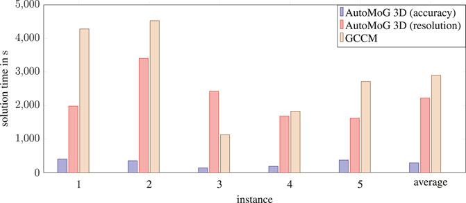
FIGURE 9. Solution time to satisfy the optimality gap of 2% for all instances and all models except the MINLP model. The MINLP model did not fulfill the optimality gap in any instance at the time limit of 48 h. Therefore, there are no solution times for the MINLP model.

The AutoMoG 3D model with comparable resolution as the generalized-convex-combination model is faster for four out of five instances and solves the pump-system synthesis problem 23% faster than the generalized-convex-combination model on average (2,224 vs 2,897 s, Figure 9). The AutoMoG 3D model has 5,500 binary variables for the pump-system synthesis problem after preprocessing and thus still 33% fewer binary variables. Still, the AutoMoG 3D model has higher accuracy with a relative model error $\overline{{ϵ}^{\text{power}}}$ of 0.1% compared to 1.0% in the generalized-convex-combination model (cf. Section. 3.1).

The MINLP model shows optimality gaps between 85 and 90% at the time limit of 48 h, showing that the MINLP model is computationally much more demanding than the MILP models in the case study.

3.3 Solution Quality of the AutoMoG 3D Model

After comparing the computational efficiency, we compare the solution quality of the same four models by analyzing the objective of the pump-system synthesis problem and the resulting design of the pump system.

3.3.1 Objective of the Pump-System Synthesis Problem

The pump-system synthesis problem minimizes the total annual cost. To compare the solution quality of the four models, we calculate their actual total annual cost. We define the actual total annual cost as the cost that occurs if we fix the solution of a model and recalculate the total annual cost of this solution in the MINLP model.

The synthesis problems provide the chosen pumps, their sizes, and their operating points. We fix the pumps, their sizes, and their operating status for each time step in the MINLP model. Then, we recalculate the MINLP model with the actual nonlinear power functions to obtain the actual total annual cost of each model and instance (Figure 10).

FIGURE 10

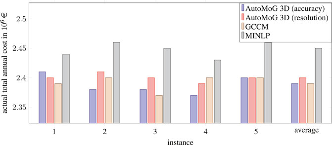
FIGURE 10. Actual total annual cost for all instances and models. The actual total annual cost is determined by fixing the solution of every model and recalculating the total annual cost of this solution in the MINLP model. All MILP models find a better solution in all instances than the MINLP model finds within 48 h.

For each instance, the three MILP solutions have lower actual total annual costs than the best feasible MINLP solution at the time limit of 48 h. In the following, we compare the MILP solutions with each other. The actual total annual costs of the three MILP models do not differ more than 1% for any instance. None of the MILP models provides solutions with a lower actual total annual cost for all instances. Thus, none of the MILP models can be claimed to systematically identify solutions with lower actual total annual cost than the other MILP models. All MILP models show a comparable solution quality (Figure 10). However, the solutions of the AutoMoG 3D models are found faster (Figure 9). To demonstrate the need for accurate models, we also modeled all pumps with only one affine region and solved the synthesis problem with these models. In that case, the actual total annual cost increases by 10% to 2.62 × 10⁶ € on average. This result shows that more accurate models like the former used MILP models are necessary for a high solution quality.

In summary, AutoMoG 3D generates the models of the pump system automatically in 1 min and provides computationally more efficient models compared to the generalized-convex-combination model. Still, the solution quality of the AutoMoG 3D models is as high as the solution quality of the generalized-convex-combination model.

3.3.2 Design of the Pump-System

Table 1 shows the resulting pump system design for all instances and models. The designs resulting from the three MILP models consist of more fixed-speed pumps than variable-speed pumps in almost every instance. At least one variable-speed pump is chosen for each instance. This result seems meaningful: Fixed-speed pumps operate more efficiently at nominal volumetric flow rate than variable-speed pumps since variable-speed pumps need frequency converters that cause efficiency losses. At the same time, fixed-speed pumps operate inefficiently at variable volumetric flow rates since the volumetric flow rate is reduced by throttling the pressure difference. Thus, the pump system operates such that the variable-speed pumps balance the fluctuations of the volumetric-flow demand. Thereby, the variable-speed pumps allow the fixed-speed pumps to operate efficiently at nominal volumetric flow rate.

TABLE 1

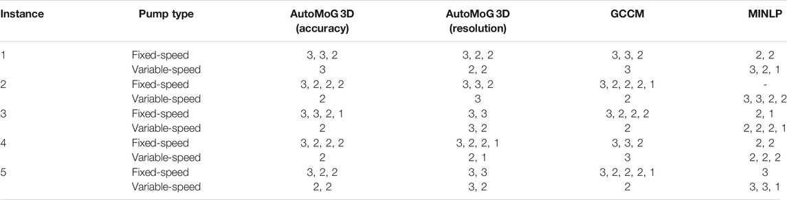
TABLE 1. Design of the pump system for all instances and models. The table lists the nominal volumetric flow rate of each installed pump. The nominal volumetric flow rate ${\dot{V}}^{\text{nom}}$ of each installed pump is presented in 1,000 m³ h⁻¹.

The designs from the MINLP model consist of more variable-speed pumps than fixed-speed pumps in every instance. These solutions of the MINLP are feasible but lead to higher total annual costs (Figure 10).

4 Conclusion

The AutoMoG 3D method is proposed for the multidimensional automated data-driven model generation of multi-energy systems. AutoMoG 3D generates MILP optimization models from measured data of multi-energy systems. AutoMoG 3D can model components with an arbitrary number of independent variables using hinging-hyperplane trees. Thus, AutoMoG 3D overcomes the main limitation of the original AutoMoG method that was limited to systems that contain components with only one independent variable. However, in general, AutoMoG 3D does not generate continuous functions of the component models.

In the case study, a real-world pump system is modeled. AutoMoG 3D needs significantly fewer piecewise-affine regions to approximate the actual functions of the pumps with comparable accuracy as the generalized-convex-combination model. AutoMoG 3D provides the model of the pump system within 1 min.

The computational efficiency and accuracy of the AutoMoG 3D model were shown by solving the pump-system synthesis problem. The AutoMoG 3D model solves 10 times faster than the generalized-convex-combination model. Still, the solution quality of the AutoMoG 3D model is the same as for the generalized-convex-combination model. The performance of the MINLP model is much worse, with an average optimality gap of 88.5% at the time limit of 48 h whereas AutoMoG 3D found a better solution in 5 min. Thus, AutoMoG 3D generates an accurate and computationally efficient model of the industrial real-world pump system.

The AutoMoG 3D method can be applied either if measured input and output data of the components are available or if the actual functions of the components are available. To enable a straightforward application of AutoMoG 3D, we are working on a Python version of the code to be released open-source. AutoMoG 3D drastically reduces the effort for both data-driven modeling and optimization. Thereby, AutoMoG 3D empowers broader applicability of MILP optimization models in real-world applications.

Data Availability Statement

The original contributions presented in the study are included in the article/Supplementary Material, further inquiries can be directed to the corresponding author.

Author Contributions

AK was involved in the Conceptualization, Methodology, Software, Validation, Investigation, Data Curation, Writing - Original Draft and Review and Editing, Visualization, Project administration, and Funding acquisition for this contribution. AH was involved in the Methodology, Software, Investigation, and Visualization. LL was involved in Conceptualization, Methodology, Writing - Review and Editing, and Visualization. AB was involved in Conceptualization, Methodology, Writing - Review and Editing, Supervision, Resources, and Funding acquisition.

Funding

This study is funded by the German Federal Ministry of Economic Affairs and Energy (Ref. no.: 03ET4068A). The support is gratefully acknowledged.

Conflict of Interest

The authors declare that the research was conducted in the absence of any commercial or financial relationships that could be construed as a potential conflict of interest.

Publisher’s Note

All claims expressed in this article are solely those of the authors and do not necessarily represent those of their affiliated organizations, or those of the publisher, the editors and the reviewers. Any product that may be evaluated in this article, or claim that may be made by its manufacturer, is not guaranteed or endorsed by the publisher.

References

Akaike, H. (1974). A New Look at the Statistical Model Identification. IEEE Trans. Automat. Contr. 19, 716–723. doi:10.1109/tac.1974.1100705

CrossRef Full Text | Google Scholar

Anderson, R., Huchette, J., Ma, W., Tjandraatmadja, C., and Vielma, J. P. (2020). Strong Mixed-Integer Programming Formulations for Trained Neural Networks. Math. Program 183, 3–39. doi:10.1007/s10107-020-01474-5

CrossRef Full Text | Google Scholar

Andiappan, V. (2017). State-Of-The-Art Review of Mathematical Optimisation Approaches for Synthesis of Energy Systems. Process. Integr. Optim. Sustain. 1, 165–188. doi:10.1007/s41660-017-0013-2

CrossRef Full Text | Google Scholar

Bahl, B., Lützow, J., Shu, D., Hollermann, D. E., Lampe, M., Hennen, M., et al. (2018). Rigorous Synthesis of Energy Systems by Decomposition via Time-Series Aggregation. Comput. Chem. Eng. 112, 70–81. doi:10.1016/j.compchemeng.2018.01.023

CrossRef Full Text | Google Scholar

Barber, C. B., Dobkin, D. P., and Huhdanpaa, H. (1996). The Quickhull Algorithm for Convex Hulls. ACM Trans. Math. Softw. 22, 469–483. doi:10.1145/235815.235821

CrossRef Full Text | Google Scholar

Baumgärtner, N., Bahl, B., Hennen, M., and Bardow, A. (2019). RiSES3: Rigorous Synthesis of Energy Supply and Storage Systems via Time-Series Relaxation and Aggregation. Comput. Chem. Eng. 127, 127–139. doi:10.1016/j.compchemeng.2019.02.006

CrossRef Full Text | Google Scholar

Bischi, A., Taccari, L., Martelli, E., Amaldi, E., Manzolini, G., Silva, P., et al. (2014). A Detailed MILP Optimization Model for Combined Cooling, Heat and Power System Operation Planning. Energy 74, 12–26. doi:10.1016/j.energy.2014.02.042

CrossRef Full Text | Google Scholar

Bonvin, D., Georgakis, C., Pantelides, C. C., Barolo, M., Grover, M. A., Rodrigues, D., et al. (2016). Linking Models and Experiments. Ind. Eng. Chem. Res. 55, 6891–6903. doi:10.1021/acs.iecr.5b04801

CrossRef Full Text | Google Scholar

Breiman, L. (1993). Hinging Hyperplanes for Regression, Classification, and Function Approximation. IEEE Trans. Inform. Theor. 39, 999–1013. doi:10.1109/18.256506

CrossRef Full Text | Google Scholar

Cozad, A., Sahinidis, N. V., and Miller, D. C. (2014). Learning Surrogate Models for Simulation-Based Optimization. Aiche J. 60, 2211–2227. doi:10.1002/aic.14418

CrossRef Full Text | Google Scholar

Ernst, S. (1998). “Hinging Hyperplane Trees for Approximation and Identification,” in Proceedings of the 37th IEEE Conference on Decision and Control (Cat. No.98CH36171) (IEEE), 1266–1271. doi:10.1109/CDC.1998.758452

CrossRef Full Text | Google Scholar

Fischetti, M., and Jo, J. (2018). Deep Neural Networks and Mixed Integer Linear Optimization. Constraints 23, 296–309. doi:10.1007/s10601-018-9285-6

CrossRef Full Text | Google Scholar

GAMS Development Corporation (2016). General Algebraic Modeling System (GAMS) Release 27.3.0[Dataset].

Google Scholar

Geißler, B. (2011). Towards Globally Optimal Solutions for MINLPs by Discretization Techniques with Applications in Gas Network Optimization, Ph.D. thesis (Nürnberg: Naturwissenschaftliche Fakultät der Friedrich-Alexander-Universität Erlangen).

Geißler, B., Martin, A., Morsi, A., and Schewe, L. (2012). “Using Piecewise Linear Functions for Solving MINLPs,” in Using Piecewise Linear Functions for Solving MINLPs (New York: Springer), 287–314. doi:10.1007/978-1-4614-1927-31010.1007/978-1-4614-1927-3_10

CrossRef Full Text | Google Scholar

Grimstad, B., and Andersson, H. (2019). ReLU Networks as Surrogate Models in Mixed-Integer Linear Programs [Dataset]. doi:10.1016/j.compchemeng.2019.106580

CrossRef Full Text | Google Scholar

Guelpa, E., Bischi, A., Verda, V., Chertkov, M., and Lund, H. (2019). Towards Future Infrastructures for Sustainable Multi-Energy Systems: A Review. Energy 184, 2–21. doi:10.1016/j.energy.2019.05.057

CrossRef Full Text | Google Scholar

Hurvich, C. M., and Tsai, C.-L. (1993). A Corrected Akaike Information Criterion for Vector Autoregressive Model Selection. J. Time Ser. Anal. 14, 271–279. doi:10.1111/j.1467-9892.1993.tb00144.x

CrossRef Full Text | Google Scholar

IBM Corporation (2017). IBM ILOG CPLEX Optimization Studio. User Guide [Dataset].

Google Scholar

ISO 50001:2018 (2018). Energy Management Systems – Requirements with Guidance for Use [Dataset].

Google Scholar

Kämper, A., Leenders, L., Bahl, B., and Bardow, A. (2021). Automog: Automated Data-Driven Model Generation of Multi-Energy Systems Using Piecewise-Linear Regression. Comput. Chem. Eng. 145, 107162. doi:10.1016/j.compchemeng.2020.107162

CrossRef Full Text | Google Scholar

Kantor, I., Robineau, J.-L., Bütün, H., and Maréchal, F. (2020). A Mixed-Integer Linear Programming Formulation for Optimizing Multi-Scale Material and Energy Integration. Front. Energ. Res. 8, 49. doi:10.3389/fenrg.2020.00049

CrossRef Full Text | Google Scholar

Katz, J., Pappas, I., Avraamidou, S., and Pistikopoulos, E. N. (2020). Integrating Deep Learning Models and Multiparametric Programming. Comput. Chem. Eng. 136, 106801. doi:10.1016/j.compchemeng.2020.106801

CrossRef Full Text | Google Scholar

Kazda, K., and Li, X. (2021). Nonconvex Multivariate Piecewise-Linear Fitting Using the Difference-Of-Convex Representation. Comput. Chem. Eng. 150, 107310. doi:10.1016/j.compchemeng.2021.107310

CrossRef Full Text | Google Scholar

Kenesei, T., and Abonyi, J.. (2015). Interpretability of Computational Intelligence-Based Regression Models. Springer Briefs in Computer Science (Cham: Springer International Publishing).

Google Scholar

Kong, L., and Maravelias, C. T. (2020). On the Derivation of Continuous Piecewise Linear Approximating Functions. INFORMS J. Comput. 32, 531–546. doi:10.1287/ijoc.2019.0949

CrossRef Full Text | Google Scholar

Mancarella, P., Andersson, G., Pecas-Lopes, J. A., and Bell, K. R. W. (2016). “Modelling of Integrated Multi-Energy Systems: Drivers, Requirements, and Opportunities,” in Power Systems Computation Conference (PSCC) (IEEE), 1–22. doi:10.1109/PSCC.2016.7541031

CrossRef Full Text | Google Scholar

Mancarella, P. (2014). MES (Multi-energy Systems): An Overview of Concepts and Evaluation Models. Energy 65, 1–17. doi:10.1016/j.energy.2013.10.041

CrossRef Full Text | Google Scholar

McBride, K., and Sundmacher, K. (2019). Overview of Surrogate Modeling in Chemical Process Engineering. Chem. Ingenieur. Technik. 91, 228–239. doi:10.1002/cite.201800091

CrossRef Full Text | Google Scholar

McKay, M. D., Beckman, R. J., and Conover, W. J. (1979). Comparison of Three Methods for Selecting Values of Input Variables in the Analysis of Output from a Computer Code. Technometrics 21, 239–245. doi:10.1080/00401706.1979.10489755

CrossRef Full Text | Google Scholar

Mitsos, A., Asprion, N., Floudas, C. A., Bortz, M., Baldea, M., Bonvin, D., et al. (2018). Challenges in Process Optimization for New Feedstocks and Energy Sources. Comput. Chem. Eng. 113, 209–221. doi:10.1016/j.compchemeng.2018.03.013

CrossRef Full Text | Google Scholar

Moretti, L., Martelli, E., and Manzolini, G. (2020). An Efficient Robust Optimization Model for the Unit Commitment and Dispatch of Multi-Energy Systems and Microgrids. Appl. Energ. 261, 113859. doi:10.1016/j.apenergy.2019.113859

CrossRef Full Text | Google Scholar

Obermeier, A., Vollmer, N., Windmeier, C., Esche, E., and Repke, J.-U. (2021). Generation of Linear-Based Surrogate Models from Non-linear Functional Relationships for Use in Scheduling Formulation. Comput. Chem. Eng. 146, 107203. doi:10.1016/j.compchemeng.2020.107203

CrossRef Full Text | Google Scholar

Pucar, P., and Sjöberg, J. (1998). On the Hinge-Finding Algorithm for Hingeing Hyperplanes. IEEE Trans. Inform. Theor. 44, 1310–1319. doi:10.1109/18.669422

CrossRef Full Text | Google Scholar

Rebennack, S., and Krasko, V. (2020). Piecewise Linear Function Fitting via Mixed-Integer Linear Programming. INFORMS J. Comput. 32, 507–530. doi:10.1287/ijoc.2019.0890

CrossRef Full Text | Google Scholar

Roll, J., Bemporad, A., and Ljung, L. (2004). Identification of Piecewise Affine Systems via Mixed-Integer Programming. Automatica 40, 37–50. doi:10.1016/j.automatica.2003.08.006

CrossRef Full Text | Google Scholar

Stoica, P., and Selén, Y. (2004). Model-order Selection. IEEE Signal. Process. Mag. 21, 36–47. doi:10.1109/msp.2004.1311138

CrossRef Full Text | Google Scholar

Thie, N., Franken, M., Schwaeppe, H., Bottcher, L., Muller, C., Moser, A., Schumann, K., Vigo, D., Monaci, M., Paronuzzi, P., Punzo, A., Pozzi, M., Gordini, A., Cakirer, K. B., Acan, B., Desideri, U., and Bischi, A. (2020). “Requirements for Integrated Planning of Multi-Energy Systems,” in 6th IEEE International Energy Conference (ENERGYCon), 696–701. doi:10.1109/ENERGYCon48941.2020.9236466

CrossRef Full Text | Google Scholar

Voll, P., Klaffke, C., Hennen, M., and Bardow, A. (2013). Automated Superstructure-Based Synthesis and Optimization of Distributed Energy Supply Systems. Energy 50, 374–388. doi:10.1016/j.energy.2012.10.045

CrossRef Full Text | Google Scholar

Wang, X., Palazoglu, A., and El-Farra, N. H. (2015). Operational Optimization and Demand Response of Hybrid Renewable Energy Systems. Appl. Energ. 143, 324–335. doi:10.1016/j.apenergy.2015.01.004

CrossRef Full Text | Google Scholar

Welsch, M., Mentis, D., and Howells, M. (2014). “Long-Term Energy Systems Planning,” in Renewable Energy Integration. Editor L. E. Jones (London: Academic Press), 215–225. doi:10.1016/B978-0-12-407910-6.00017-X

CrossRef Full Text | Google Scholar

Wilson, Z. T., and Sahinidis, N. V. (2017). The ALAMO Approach to Machine Learning. Comput. Chem. Eng. 106, 785–795. doi:10.1016/j.compchemeng.2017.02.010

CrossRef Full Text | Google Scholar

Zhang, Q., Grossmann, I. E., Sundaramoorthy, A., and Pinto, J. M. (2016). Data-driven Construction of Convex Region Surrogate Models. Optim. Eng. 17, 289–332. doi:10.1007/s11081-015-9288-8

CrossRef Full Text | Google Scholar

Zhou, K., Kılınç, M. R., Chen, X., and Sahinidis, N. V. (2018). An Efficient Strategy for the Activation of MIP Relaxations in a Multicore Global MINLP Solver. J. Glob. Optim. 70, 497–516. doi:10.1007/s10898-017-0559-0

CrossRef Full Text | Google Scholar