 Yu Liu
 Jiarui Wang
 Jiewen Deng
 Wenquan Sheng
- School of Electrical Engineering, Southeast University, Nanjing, China
Non-intrusive load monitoring has broad application prospects because of its low implementation cost and little interference to energy users, which has been highly expected in the industrial field recently due to the development of learning algorithms. Targeting at the investigation of practical and reliable load monitoring in field implementations, a non-intrusive load disaggregation approach based on an enhanced neural network learning algorithm is proposed in this article. The presented appliance monitoring approach establishes the neural network model following the supervised learning strategy at first and then utilizes the unsupervised learning based optimization to enhance the flexibility and adaptability for diverse scenarios, leading to the improvement of disaggregation performance. By verifications on the REDD public dataset, the proposed approach is demonstrated to be with good performance in non-intrusive load monitoring. In addition to the accuracy enhancement, the proposed approach is also with good scalability, which is efficient in recognizing the newly added appliance.
Introduction
In the context of the carbon neutrality plan proposed by China in the late 2020 (President of the People’s, 2020), the energy related industry is with high expectation to contribute to the realization while the power system is highlighted. For better and efficient operation, the power grid is designed to be smart, among which the transparency, that is, knowing small-grained operating data including the status of various electrical appliances, is of high value. By knowing the operation information of single appliances, energy users can understand the insights of appliance operations and help them conduct energy conservation. In addition, the power companies may extract valuable information through electric appliance data mining and introduce corresponding measures, leading to saving electricity up to 14% (Ehrhardt et al., 2010). Therefore, providing users with appliance status information and furthermore the energy saving and cost reduction solutions has become one of the important business models in the future. This is the challenge and also opportunity for power companies and many integrated energy service providers in the context of energy digitization and information transformation. The detailed appliance monitoring is one of the effective means to support such revolution (Guo et al., 2021).
There are two implementation methods for appliance monitoring, namely, the intrusive appliance monitoring (ILM) and the non-intrusive appliance monitoring (NILM). The former focuses on the hardware by installing sensors and chips on each appliance to monitor each device separately. Meanwhile, NILM focuses on software algorithms using power data from the service panel to analyze the resident’s internal appliance operating status (HART, 1992). Considering that the sensor-based monitoring scheme is expensive, NILM is highly welcomed by energy users and becomes the research front in both academic and industrial fields.
NILM was put forward in the 1990’s by professor Hart G. W. from MIT (HART, 1992). Since the initial NILM has a high computational complexity and low accuracy, it did not attract much attention at that time. In recent years, due to the rapid development of computer science, especially the widespread use of deep learning for pattern recognition, NILM has now regained the attention of scholars and has become a research hotspot. Currently, non-intrusive appliance monitoring is mainly divided into two categories based on diverse sampling rates, that is, low-frequency and high-frequency. The information utilized in low-frequency data mainly includes current, voltage, power, etc. Because of the simplicity, the low-frequency data may lead to some problems such as inaccurate performance. Meanwhile, the high-frequency data usually contain more information, such as current harmonics, voltage–current trajectories, and high-frequency transient waveforms (Cox et al., 2006). Although the results of high-frequency data analysis are usually more accurate, the high requirements for monitoring equipment show a cost disadvantage in comparison with low-frequency data analysis. From the view of practical applications, the low-frequency data–based solutions become more and more attractive considering the industrial aspect and therefore are focused in our work.
For valid applications of NILM technology, the credible load disaggregation is the premise. To address the reliable appliance monitoring, various NILM solutions have been proposed. First, some mathematical models have been explored, such as fuzzy model (Lin and Tsai, 2014), graph signal processing (He et al., 2018), linear programming model and (Liu et al., 2020). The fuzzy model obtains the membership degree of each sample signal to all appliance centers by optimizing the objective function, thereby determining the appliance category of sample signals to achieve the purpose of automatically identifying sample data (Lin and Tsai, 2014). Meanwhile, graph signal processing first establishes an undirected graph based on the signal simple, then groups the on/off events for appliances, and finally defines an optimization problem to find the signal with a minimum variation (He et al., 2018). Linear programming model treats NILM problem as an optimization and forms a multi-feature objective function to realize appliance decomposition and recognition for different electrical appliances (Liu et al., 2020). Although some achievements have been realized by mathematical model-based research studies, there still exist some limitations. The most prominent is that most of these explorations are optimization based, resulting in the low scalability of the formulation and the high dependency of the algorithms. Therefore, the disaggregation performance is highly scenario dependent, and the model is required to be tuned for the practical applications. However, the rise of deep learning algorithms has provided some effective ways to overcome these obstacles, and hence, a number of research studies have been investigated. The hidden Markov model (HMM) (Kolter and Jaakkola, 2012) is a typical category of these studies, where a double random process combing the appliance states and explicit random functions is utilized to establish the operation series. Furthermore, neural networks (NNs) have been combined with HMMs in a study by Yan et al. (2019), where the emission probabilities of the HMM are modeled by a Gaussian distribution for the state representing the single appliance and by a DNN for the state representing the aggregated signal. By the above investigations, the high potential of deep learning approaches in the NILM problem is demonstrated.
At present, deep learning in non-intrusive appliance monitoring learning algorithms can be roughly divided into three categories, that is, supervised algorithms (Liu et al., 2019a), unsupervised algorithms (Li and Dick, 2019), and semi-supervised algorithms (Zoha et al., 2012). Supervised algorithms can learn from training data or can establish a model and then speculate a new instance based on this model. It has the advantages of simple implementation, fast calculation speed, small storage space, and high accuracy of analysis results (Liu et al., 2019a). However, there are some problems. For example, when the spatial characteristics are large, the logistic regression performance is poor. There are also some disadvantages such as under-fitting or over-fitting and poor self-learning ability. The unsupervised algorithm refers to a data processing method that classifies samples through data analysis of many samples of the research object without category information. It has strong self-learning ability and new data can be directly added to the data set without retraining, but it also has the disadvantages of low accuracy of analysis results (Kelly and Knottenbelt, 2015). Semi-supervised learning uses a large amount of unlabeled data and simultaneously uses labeled data for pattern recognition, and hence, it is considered as the most promising learning algorithm branch. However, the research on semi-supervised regression problems is relatively limited.
Among all the reviewed deep learning approaches, the neural networks are highlighted due to their outstanding performance. In addition to Bonfigli et al. (2018) where NNs are employed for the improvement of NILM performance, there are many research publications discussing the advantages of neural networks in enhancing NILM. The literature Andrean et al. (2018) is an early literature to solve the NILM by using NNs, where the studies named neural NILM are proposed at the first stage and the related research studies are inspired. Bonfigli et al. (2018) proposed a neural network-based approach for non-intrusive harmonic source identification. In this approach, NNs are trained to extract important features from the input current waveform to uniquely identify various types of devices using their distinct harmonic signatures. In order to be suitable for a specific problem, some NN approaches are modified for diverse NILM applications. An additional optimization is proposed by Faustine and Pereira (2020) to be embedded into the NILM formulation, forming the noise reduction self-encoding method. As research studies go further, more and more investigations have been reported in neural NILM problems. (Tan et al., 2011) proposed the convolutional neural network (CNN)-based multi-label learning approach, which links multiple appliances to an observed aggregate current signal. The approach applies the Fryze power theory to decompose the current features into active and non-active components and use the Euclidean distance similarity function to transform the decomposed current into an image-like representation, which achieves remarkable progress. (Liu et al., 2019b) proposed a general appliance recognition model based on the convolutional neural network. The parameters do not depend on the appliances category, and a time series of 0 and 1 can be obtained to represent the switching state of a single appliance. In a study by Monteiro et al. (2021), the problem of identifying the electrical loads connected to a house is investigated, and a system capable of extracting the energy demand of each individual device is proposed. The whole study is NILM based, and the disaggregation is CNN formulated, achieving the simultaneous detection and classification. Although proved by so many studies, CNN-based solutions have certain disadvantages that the model is usually complicated, leading to the decreased practicability. Meanwhile, the recurrent neural network (RNN) is also widely concerned in NILM, such as (Xue and Guo, 2016), where an RNN model is utilized to extract the appliance characteristics of the steady-state section as the model input for identification after the event is detected. However, in the process of large sample data training, the RNN model shows a limitation defined as a phenomenon of “gradient disappearance”. To overcome the difficulties of RNN in learning long-term dependencies, a 1D CNN-based approach is proposed in a study by Figueiredo et al. (2014), and the NILM problem is solved by considering the electrical current signals and using Long Short-Term Memory (LSTM) neural networks. Although a better performance is achieved, the high complexity infers to the impossibility of applying in field measurements by these approaches. As seen, the neural NILM is highlighted by building a multi-layer perceptron with multiple hidden layers. Through layer-by-layer training, the signal features of each layer are extracted, and finally, the underlying features are combined to form more abstract high-level features to realize the prediction and classification of data objects (Zhou et al., 2018). The only disadvantage is the algorithmic complexity. Understanding this, some investigations focusing on complexity reduction have been conducted, such as Ciancetta et al., (2021), where the simplest neural network, that is, back propagation neural network (BPNN), is used to realize load identification using the sudden change value of active power and corresponding odd harmonics only. By verifying the effectiveness of BPNN in NILM problems, it is possible to deploy such a deep learning approach for practical applications.
However, toward the practical applications of NILM, multiple new concerns emerge in addition to the high accuracy requirements. First, the deployed approach is expected to be with self-learning ability, that is, it is capable of adapting to diverse scenarios. Second, the algorithm complexity of the applied approach should be acceptable, which is possible to be allocated on smart meters. Last but not least, it would be really practical if the newly added appliance can be addressed with guaranteed performance.
In order to address the above problems, this article utilizes the unsupervised learning-based optimization to enhance the supervised learning-based NN-NILM model, while the corresponding solution is proposed to address the newly added appliance. First, the basic appliance disaggregation model is established based on the clustering oriented BPNN learning framework, where both adaptability and simplicity are achieved. Considering the deficient samples of newly added appliance, an unsupervised learning-based optimization scheme is proposed, which combines the large samples of original appliances and small samples of unknown appliance to reconstruct the learning network to achieve the reliable disaggregation. By implementing the proposed approach, the inherent problems of neutral networks, such as insufficient fitting, over-fitting, and insufficient promotion capabilities, are all alleviated, leading to the improvement of NILM with high accuracy and flexible scalability. The comprehensive verifications are investigated on the REDD public dataset, and the results demonstrate the effectiveness of our work. In addition to addressing the newly added appliance, the proposed approach also provides a reliable NILM solution with high precision and robustness, leading to the practical NILM applications.
The main contribution of this study is the presentation of a practical NILM solution with reliable accuracy, adaptive flexibility, and high scalability. In other words, the presented NILM approach can be adaptive to diverse practical application scenarios, even addressing the newly added appliance without sufficient information. Such contribution fills a research gap in related field. Detailed technical contributions can be summarized as follows:
A practical and adaptive NILM formulation model is established based on the BP neural network, of which the parameter settings are following the supervised learning scheme.
An unsupervised learning based optimization is utilized on the presented NILM model to improve the scalability and robustness of the approach.
Combining the unsupervised learning based optimization with the supervised BPNN model, the proposed NILM solution is able to identify the newly added appliances, while an important research gap is filled.
The presented model and method are verified via a public dataset. In addition to the high precision of load disaggregation, all the proposed potentials are demonstrated to be valid.
The rest of this article is organized as follows. The methodologies are discussed in the Methodology section, including the supervised NILM model based on BPNN and unsupervised optimization based enhancement. The Results and Discussions section illustrates our results and discussions in detail. Conclusions are drawn in the Conclusion section.
Methodology
Basic Principles of Neural Networks
Artificial Neuron Model
Artificial neuron is the basic element of a neural network, and its principle can be represented by Figure 1. The neuron model in the Figure 1 is called the MP model (McCulloch–Pitts Model), also known as a processing element (PE) of the neural network.
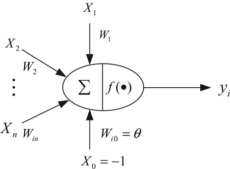
FIGURE 1. The principle of the artificial neuron model.
In Figure 1,
where neti is the net activation of the neuron i.
If the threshold is regarded as the weight Wi0 of an input x0 of neuron i, the above formula can be simplified to
If X is used to represent the input vector and W is used to represent the weight vector, that is,
then the output of the neuron can be expressed in the form of vector multiplication as
By applying a so-called activation function or transfer function f(.) on neti, the final output yi can be expressed as
If the net activation net of a neuron is positive, the neuron is said to be in an activated state or in a state of fire. If the net activation
Neural Network Models
A neural network is a network composed of many interconnected neurons, of which the feed-forward network is widely used. This kind of network only has a feed signal during the training process, and during the classification process, the data can only be sent forward until it reaches the output layer. There is no backward feedback signal between the layers, so it is called a feed-forward network. The perceptron and BP neural network belong to this type.
For a three-layer feed-forward neural network, if X is used to represent the input vector of the network, W1, W2, and W3 represent the connection weight vectors of each layer of the network, and F1, F2, and F3 represent the activation functions set of the three layers of the neural network, then the output vector Y1 of the first layer of neurons in the neural network is
The output of the second layer Y2 is
The output of the final layer Y3 is
If the activation functions are all linear functions, then the output Y3 of the neural network will be a linear function of the input X. However, the NILM problem leads to the approximation of higher order functions; therefore, an appropriate nonlinear function should be selected as the activation function.
The BP network has a strong nonlinear mapping ability, and theoretically, a three-layer BP neural network can approximate any nonlinear function. So BPNN is extremely appropriate for our NILM problem. The typical three-layer BP neural network model is shown in Figure 2A.
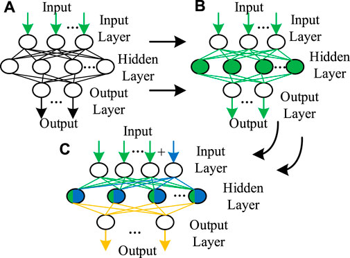
FIGURE 2. Three-layer BP neural network model and enhancement: (A) Typical model, (B) NILM featured model, (C) Enhanced NILM model addressing newly added appliance.
NILM Algorithm by Enhanced Neural Network
The Basic Model of NILM
The main idea of the NILM system is to identify the power consumption of individual appliances in a house based on the analysis of the aggregated data measured from a single meter. The whole formulation can be expressed as
where P is the aggregated data measured from a meter, Pi is the load signature of ith appliance, and e0 is the error generated. Note that the data from smart meter can be real power, reactive power, harmonics, or the combination of these electric features. Since we are targeting the practical applications, only real power and reactive power are utilized in the following discussions, that is, P denotes power. Nevertheless, the proposed approach is compatible with other feature utilizations.
BPNN Based NILM
For preparation of integrating the BPNN model into NILM formulation, the first step is to convert the measured data from a smart meter to be adequate for the BPNN input. Therefore, a normalization is required for the power matrix obtained from the entrance meter,
where P is the power matrix containing all the measured power from the meter. Pnorm is the normalized power matrix of P and also the input of BPNN. Pmin and Pmax are, respectively, the minimum power and the maximum power after traversing the measured power matrix.
Originally, we have a typical BP neural network with three layers as seen in Figure 2A. Once the processed data matrix enters the neural network as a training matrix, a non-intrusive load monitoring network following supervised learning is established, as illustrated in Figure 2B. To be specific, the network error square is used as the objective function, and the gradient descent method is used to optimize the problem. The parameters of the learning algorithm are adjusted by the validation set or cross-validation. The detailed implementations of constructing the adaptive BPNN for NILM are shown in Figure 3. After implementing the procedures, the internal parameters of the BP neural network, especially the hidden layer, have been changed and also customized with the diverse input data. Therefore, the proposed model is highly adaptive to the input data, and such a supervised learning scheme is welcomed by a practical NILM problem, where the deployed monitoring can be self-adapting to diverse household scenarios.

FIGURE 3. Method flow of BPNN based NILM.
Enhanced BPNN Based NILM
Even using a successfully trained neural network for appliance monitoring, the problem of network failure occurs due to the newly added appliances. Because there are new appliance features in the appliance clusters that have not been learned by the supervised neural network, the unsupervised learning-based scheme is required to explore the signatures of new features based on the insufficient samples. Here, the adaptive K-means clustering algorithm is used to iteratively address the newly added appliance for each target clustering center. First, the algorithm selects K points from the given dataset, where each point represents the initial cluster center. Then, calculate the Euclidean distance of each remaining sample to these cluster centers, and classify it into the cluster closest to it. Finally, recalculate the average value of each cluster. The whole process is repeated until the square error criterion function reaches the smallest (Wang et al., 2019). The square error criterion is defined as
where K is the number of clusters,
where dist(m,x) is the Euclidean distance function, calculating the Euclidean distance between point m and x. x
As seen from Eq. 11, this algorithm considers that clusters are composed of objects that are close to each other, so it makes the final goal to obtain compact and independent clusters. For practical implementation, it is important to determine the number of centers K. In our NILM problem, the method for determining the initial K value is as follows. Assume that the original N appliances are operating independently, and there are M appliances that may operate at the same time. Once we have a newly added appliance, the number of cluster centers is
In the newly added clusters, the cluster center with the lowest power value is the rated feature center of the newly added appliance. Consistently, the K-means clustering algorithm can also obtain the new appliance action time stamp and then reconstitute the training data, including the electric features, switching action, and timestamp. In order to guarantee the effectiveness of the rated feature center, the following verification is conducted:
where Mo and Mn are, respectively, the original cluster sets and newly added cluster sets. mna is the rated feature center of the newly added appliance. mo,i
Following the above strategies, the detailed procedures addressing the newly added appliance are illustrated in Figure 4. By introducing a larger closed loop feedback as shown on the right, the approach handling the newly added appliance is embedded into the BPNN framework. The key change of the neural network is shown in Figure 2C. By modifying the training matrix to change the constraints of the neural network and reconstruct it, the neural network can learn the rated features of the newly added appliance by itself. Specifically, the internal structure of the BP neural network is enhanced from two aspects. First, the input layer is supplemented with new neurons to handle the newly added appliance. Second, the parameters of the hidden layer are totally tuned based on the additional information by the newly added appliance. Correspondingly, the data flow after the hidden layer changes to take the new appliance feature into consideration. Based on the above analysis, the BPNN performs well even with insufficient data of newly added appliance. Such a strategy follows an unsupervised strategy and uses the K-means algorithm as the basic approach, so defined as K-means based unsupervised optimization. By enhancing the BPNN through K-means based unsupervised optimization, the scalability of the neural network NILM method has been improved. Besides, via the evolution process as shown from (a), (b), and (c) in Figure 2, it is clearly seen that the key ideas and solutions of incorporating the concerned problems in the BPNN-based NILM formulations.
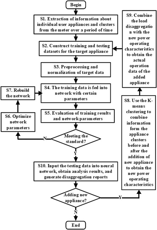
FIGURE 4. The method flow of enhanced NILM with newly added appliance.
Results and Discussions
Data Preparation
In order to verify the effectiveness of the proposed strategy and approach, this article uses the data set generated based on the REDD data to conduct case studies. The data composition of the REDD low-frequency dataset is the power under 1 Hz for integral signals and 0.2–0.3 Hz for individual appliances. To be consistent, the data for individual appliances are complemented to be 1 Hz. Considering the different operating states and the possible power fluctuations, two scenarios with different complexities are prepared to analyze the proposed study. Dataset A is with a relatively simple appliance operating condition. It runs for 21 days and has seven independent appliances under a regular operation mode, as well as one newly added appliance. Dataset B is considering a more complicated operation situation, also running for a total of 21 days and with six independent appliances, as well as one newly added appliance. However, the appliances are operating randomly with more than 60 different operation combinations.
General NILM Results
In order to fully evaluate the performance of the study, this article selects four metrics, that is, precision, recall rate, F1 score, and average absolute error as evaluation indicators. The specific calculation of metrics (Barsim et al., 2014) is as follows:
where PRE represents the precision. REC represents the recall rate. F1 represents the F1 score, also known as the balanced F score. TP represents the total number of the sequence points that the electrical appliance is actually working and the disaggregation result is also working. FP represents the number of sequence points that the electrical appliance is actually working but the result is in a non-working state. FN represents the total number of sequence points, which indicate that the electrical appliance is actually not working but the model decomposition result is in the working state. yt represents the true power of the electrical appliance at a time t.
First, results and discussions are provided focusing on the dataset A. Through multiple experiments for the dataset A, the disaggregation results without the consideration of the newly added appliance are shown in Table 1, while Table 2 shows the results by the complete strategy and approach proposed in this study. As seen, after the new appliance is added, the new network obtained by the proposed algorithm has good performance in accuracy, recall rate, and balanced F1 score. Comparing with the approach that BPNN without unsupervised optimization, we can see the remarkable enhancement by the proposed study. The load disaggregation results are reliable and desired with a new appliance considered in the household.
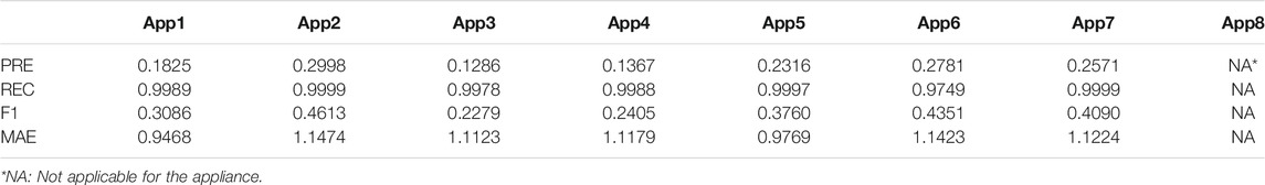
TABLE 1. Results of BPNN without unsupervised optimization for dataset A.
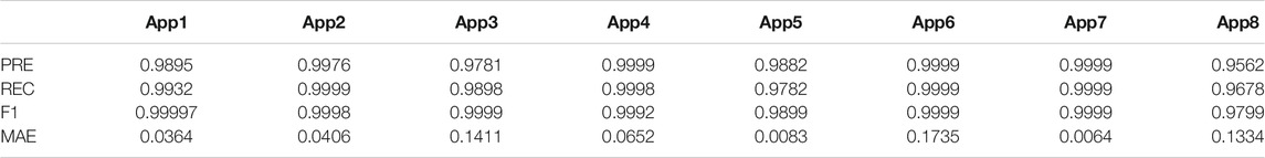
TABLE 2. Results of BPNN with unsupervised optimization for dataset A.
Because the appliance operation mode of dataset A is relatively simple, the parameters calculated in the BPNN have a good degree of fit. To test the robustness of the algorithm, data set B with complex appliance operation mode is used for analysis again. Table 3 illustrates the disaggregation performance for dataset B by implementing our approach. Although the precision, F1 score, and MAE parameters have been reduced to a certain extent, the proposed approach is still effective in recognizing the newly added appliance. In detail, the recall rates keep in a high level, while the balanced F1 scores are almost all over 0.6. Such results are desirable since we only take real and reactive power as our load signatures and try to disaggregate the appliances under complicated operation modes. As to the power error, Table 1 shows that the traditional BPNN method has a large MAE. By introducing the enhancement in Table 2, the MAE becomes very small, indicating the effectiveness of energy consumption monitoring. Such efficiency, although reduced, can still be found for complicated operation scenarios, as the results seen in Table 3.
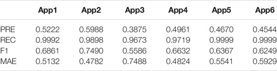
TABLE 3. Results of BPNN with unsupervised optimization for dataset B.
Combining Table 1, 2, and 3, the average metrics for different scenarios are visualized in Figure 5. It can be seen that the traditional BPNN without unsupervised optimization performs worst. The proposed BPNN solution with unsupervised optimization is compatible of handling both datasets A and B. Although a slight decrease is seen via some metrics, the disaggregation results are reliable from the view of whole household energy consumption.

FIGURE 5. Comparison of analysis results.
To give a comprehensive illustration of our study, some appliances are selected for extended discussions. Energy disaggregation results for App1 and App8 from dataset A are illustrated in Figure 6. As shown by the green line, when the BPNN without unsupervised optimization encounters the appliance clusters with the new appliance, the analysis performance will be greatly reduced. As shown by the red line, the BPNN with unsupervised optimization in this article has the better capability to analyze all the appliances, including the newly added appliance.
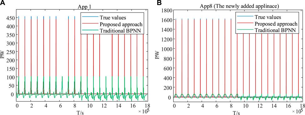
FIGURE 6. Energy disaggregation results by diverse approaches (A) App1, (B) App8 (the newly added appliance).
Energy disaggregation results of App1 from dataset B is also selected for illustration, as shown in Figure 7. We can see that the algorithm still has a certain analytical ability and can clearly distinguish the operating time of each appliance and the approximate operating information.
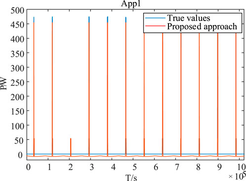
FIGURE 7. Energy disaggregation results of App1 from dataset B.
NN Model Performance
In order to investigate the insights of NN performance in our study, details are explored. In above cases, the initial neuron number of the hidden layer is 3, the initial learning rate is 0.001, and the maximum number of failures is fixed at 10. In addition, for the part of network training, the elastic gradient descent method is used. After the training stage, the established network is compared with the required error to determine the whether it is valid. If not satisfied, the coordinate axis descent method is activated to optimize the network parameters, rebuild the network for retraining, and analyze the training results again until the accuracy requirements are met. In our NILM problem, the training results are shown in Figure 8.
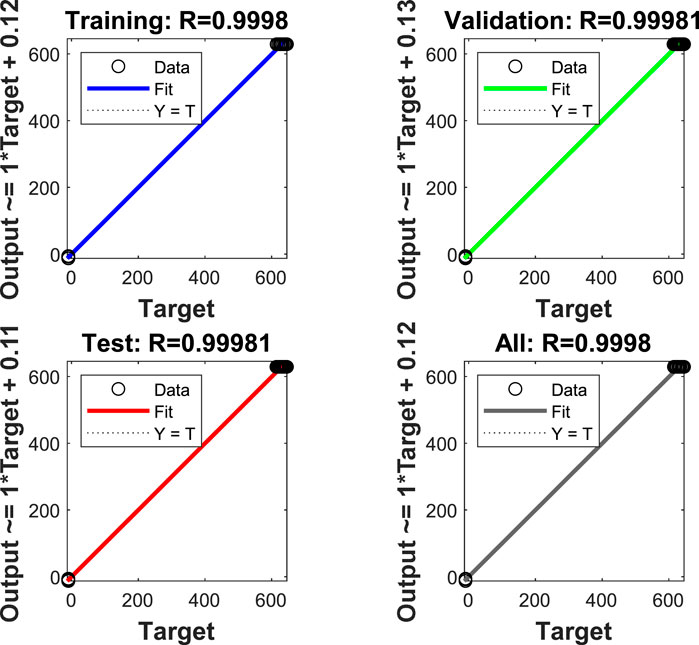
FIGURE 8. The training results of the neural network.
Using this network to decompose each appliance data, we can get the operation status of each appliance. We draw the disaggregation diagram of each appliance obtained through neural network analysis with the real data of each appliance in a chart for comparison, as shown in Figure 9 for dataset A, and we can see that the disaggregated results are now very close to the true values. The illustrated results suggest the effectiveness of the established network.
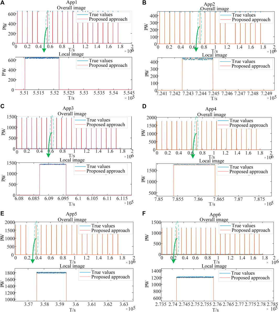
FIGURE 9. Load disaggregation performance of the trained neural network for dataset A: (A) App1, (B) App2, (C) App3, (D) App4, (E) App5, and (F) App6.
Since applying a more complex appliance running dataset is an effective way to test the generalization and robustness of the algorithm, the load disaggregation performance of the trained neural network for dataset B is analyzed and shown in Figure 10. Although there is a certain error for the appliance power tracking, it is acceptable within a small range. Therefore, the neural network has strong generalization ability and good robustness, even for complex appliance operation data, which is desired in the NILM problems.
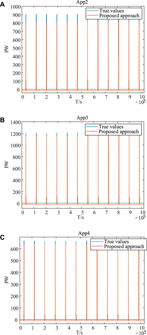
FIGURE 10. Load disaggregation performance of the trained neural network for dataset B: (A) App2, (B) App3, and (C) App4.
Handling the Newly Added Appliance
Extensive discussions on dataset A are presented here to show how the proposed approach handles the newly added appliance. Originally, there are seven appliances in the household system, while the App7 is a long-run appliance. By training, the clustered operation feature centers are illustrated in Figure 11, where there are total 16 clusters for these household operations.
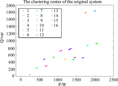
FIGURE 11. The appliance clustering feature center of the original system.
When a new appliance is added, the function of the original network will fail. As a result, the disaggregation results will differ remarkably from the true operating power. For example, Figure 12 shows the large disaggregation errors of App1 and App3 under a certain time period.
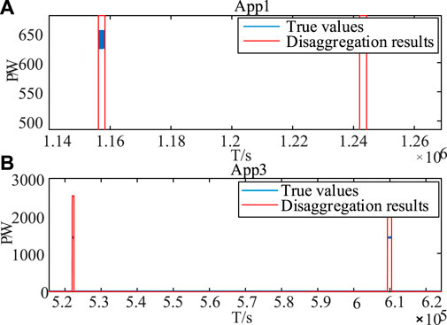
FIGURE 12. Disaggregation errors with original cluster centers: (A) App1 (B) App3.
Considering the newly added App8, through the calculations by Eqs 10–13, Figure 13 below shows the clustering results of the new system, where there are total 24 cluster centers and eight of them are the new centers.
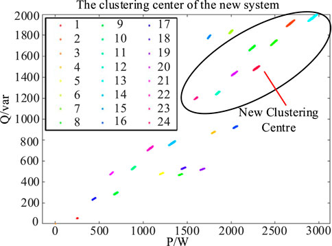
FIGURE 13. The new system cluster centers.
The corresponding clustering centers are digitized in Table 4, where the new centers are listed on the right. As seen, Eq. 13 not only provides an indicator to check the validity of the rated feature of the newly added appliance but also helps to determine the optimal clustering centers. It plays a vital role in the proposed unsupervised learning enhancement.
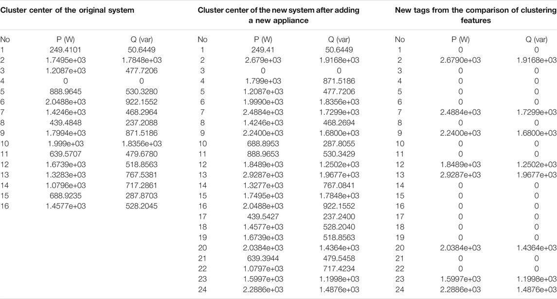
TABLE 4. The results of the K-means clustering algorithm.
By extracting the newly added appliance information from Table 4, the rated operating power of the new appliance in the new system can be calculated, and the new BPNN-based NILM system can be constructed. Figure 14 below shows the disaggregation results of the new appliance by the newly constructed network.
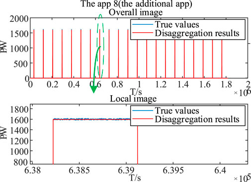
FIGURE 14. The disaggregation results of the new appliance by the newly constructed network.
As seen from Figure 14, by implementing the proposed approach, the newly added appliance can be accurately tracked under the NILM framework. However, if there are two or more new appliances, following discussions can be noticed. If the new appliances are added one by one, our system is still effective in recognizing them, since after a period of time the newly added appliance will change to be the conventional appliance. If they are added together, our approach can only tell that multiple electrical appliances have been added but cannot build the learning model for each in the neural networks. This is indeed the true challenge we will focus on in the future. Nevertheless, such a scenario does not affect our contribution because current NILM studies are mostly targeting at the residential power monitoring, where the total number of monitored appliances is limited. It is very unusual for a house to add two new household appliances at the same time, so such a capability does not influence our contribution to the practical NILM applications.
Conclusion
Toward the practical non-intrusive load disaggregation in field measurements, especially to tackle the newly added appliance with deficient samples in the NILM field, the BPNN-based solution is thoroughly investigated and improved in this article. Specifically, a deep learning-based NILM approach is proposed, where the model is established based on the supervised BP neural network and enhanced by the unsupervised optimization, and the solution is provided with adaptive scalabilities. By the joint optimization design based on large samples of original appliances and small samples of newly added appliances, the brand new features of unknown appliances are effectively handled by the enhanced BPNN model, leading to the capability of recognizing the out-of-range appliance. In addition to the desired accuracy, the proposed approach is demonstrated to be with high reliability and scalability, proving to be a feasible solution in the future practical NILM applications.
Data Availability Statement
The raw data supporting the conclusions of this article will be made available by the authors, without undue reservation.
Author Contributions
YL: conceptualization, writing—review and editing, funding acquisition, and supervision. JW: writing—original draft, writing—review and editing. JD: software and validation. WS: formal Analysis. PT: methodology.
Funding
This work was supported in part by the National Natural Science Foundation of China under Grant 51907024.
Conflict of Interest
The authors declare that the research was conducted in the absence of any commercial or financial relationships that could be construed as a potential conflict of interest.
Publisher’s Note
All claims expressed in this article are solely those of the authors and do not necessarily represent those of their affiliated organizations, or those of the publisher, the editors and the reviewers. Any product that may be evaluated in this article, or claim that may be made by its manufacturer, is not guaranteed or endorsed by the publisher.
References
Andrean, V., Zhao, X.-H., Teshome, D. F., Huang, T.-D., and Lian, K.-L. (2018). A Hybrid Method of Cascade-Filtering and Committee Decision Mechanism for Non-intrusive Load Monitoring. IEEE Access 6, 41212–41223. doi:10.1109/access.2018.2856278
Barsim, K. S., Wiewel, F., and Yang, B. (2014). On the Feasibility of Generic Deep Disaggregation for Single-Load Extraction. In The 4rd International Workshop on Non-intrusive Load Monitoring. Washington, America, 1–5.
Bonfigli, R., Felicetti, A., Principi, E., Fagiani, M., Squartini, S., and Piazza, F. (2018). Denoising Autoencoders for Non-intrusive Load Monitoring: Improvements and Comparative Evaluation. Energy and Buildings 158, 1461–1474. doi:10.1016/j.enbuild.2017.11.054
Ciancetta, F., Bucci, G., Fiorucci, E., Mari, S., and Fioravanti, A. (2021). A New Convolutional Neural Network-Based System for NILM Applications. IEEE Trans. Instrumentation Meas. 70, 1501112. doi:10.1109/tim.2020.3035193
Cox, R., Leeb, S. B., and Shaw, S. R. (2006). Transient Event Detection for Nonintrusive Load Monitoring and Demand Side Management Using Voltage Distortion. In Twenty-First Annual IEEE Applied Power Electronics Conference and Exposition. Dallas, TX, USA: IEEE.
Ehrhardt, K., Donnelly, K., and Lait, J. A. (2010). Advanced Metering Initiatives and Residential Feedback Programs: A Meta-Review for Household Electricity-Saving Opportunities. Washington DC, United State: American Council for an Energy-Efficient Economy.
Faustine, A., and Pereira, L. (2020). Multi-Label Learning for Appliance Recognition in NILM Using Fryze-Current Decomposition and Convolutional Neural Network. Energies 13, 4154. doi:10.3390/en13164154
Figueiredo, M., Ribeiro, B., and de Almeida, A. (2014). Electrical Signal Source Separation via Nonnegative Tensor Factorization Using on Site Measurements in a Smart home. IEEE Trans. Instrum. Meas. 63 (2), 364–373. doi:10.1109/TIM.2013.2278596
Guo, H., Lu, J., and Yang, P. (2021). Review on Key Techniques of Non-intrusive Load Monitoring. Electric Power Automation Equipment 41 (1).
Hart, G. W. (1992). Nonintrusive Appliance Load Monitoring. Proc. IEEE 80 (12), 1870–1891. doi:10.1109/5.192069
He, K., Stankovic, L., Liao, J., and Stankovic, V. (2018). Non-Intrusive Load Disaggregation Using Graph Signal Processing. IEEE Trans. Smart Grid 9 (3). doi:10.1109/tsg.2016.2598872
Kelly, J., and Knottenbelt, W. (2015). Neural NILM. In Proceedings of the 2nd ACM International Conference on Embedded Systems for Energy-Efficient Built Environments. New York, NY, USA: Association for Computing Machinery, 55–64. doi:10.1145/2821650.2821672
Kolter, J. Z., and Jaakkola, T. (2012). “ Approximate Inference in Additive Factorial HMMS with Application to Energy Disaggregation”, in Proceedings of the 15th International Conference on Artificial Intelligence and Statistics, Journal of Machine Learning Research. La Palma, Spain 22, 1472–1482.
Li, D., and Dick, S. (2019). Residential Household Non-intrusive Load Monitoring via Graph-Based Multi-Label Semi-supervised Learning. IEEE Trans. Smart Grid 10 (4), 4615–4627. doi:10.1109/tsg.2018.2865702
Lin, Y.-H., and Tsai, M.-S. (2014). Non-Intrusive Load Monitoring by Novel Neuro-Fuzzy Classification Considering Uncertainties. IEEE Trans. Smart Grid 5 (5), 2376–2384. doi:10.1109/tsg.2014.2314738
Liu, H. Y., Shi, S. B., and Xu, H. X. (2019). A Non-intrusive Load Identification Method Based on RNN Model. Power Syst. Prot. Control. 47 (13), 162–170.
Liu, Q., Kamoto, K. M., Liu, X., Sun, M., and Linge, N. (2019). Low-Complexity Non-intrusive Load Monitoring Using Unsupervised Learning and Generalized Appliance Models. IEEE Trans. Consumer Electron. 65 (1), 28–37. doi:10.1109/tce.2019.2891160
Liu, S., Liu, Y., Gao, S., Guo, H., Song, T., Jiang, W., et al. (2020). Non-intrusive Load Monitoring Method Based on PCA-ILP Considering Multi-Feature Objective Function. IEEE Trans. Consumer Elect. 2020, 1000–7229.
Monteiro, R. V. A., de Santana, J. C. R., Teixeira, R. F. S., Bretas, A. S., Aguiar, R., and Poma, C. E. P. (2021). Non-intrusive Load Monitoring Using Artificial Intelligence Classifiers: Performance Analysis of Machine Learning Techniques. Electric Power Syst. Res. 198, 107347. doi:10.1016/j.epsr.2021.107347
President of the People's Republic of China (2020). Carrying on the Past and Opening up a New Journey of Global Response to Climate Change. Available at: http://www.gov.cn/gongbao/content/2020/content_5570055.htm.
Tan, P. N., Steinbach, M., and Kumar, V. (2011). Introduction to Data Mining. FAN Ming, FAN Hongjian. Beijing: People Post Press.
Wang, K., Zhong, H., Yu, N., and Xia, Q. (2019). Nonintrusive Load Monitoring Based on Sequence-To-Sequence Model with Attention Mechanism. Proc. CSEE 2019, 0258–8013.
Xue, F. X., and Guo, D. Z. A Survey on Deep Learning for Natural Language Processing. Acta Automatica Sinica, 2016, 42(10): 1445–1465.
Yan, X., Zhai, S., Wang, F., and He, G. (2019). Application of Deep Neural Network in Non-intrusive Load Disaggregation. Automation Electric Power Syst. doi:10.7500/AEPS20180629004
Zhou, M., Song, X., and Tu, J. (2018). Residential Electricity Consumption Behavior Analysis Based on Non-intrusive Load Monitoring. Power Syst. Tech. 42 (10), 3268–3274.
Keywords: unsupervised learning, NILM, neural network, BP – back propagation algorithm, electricity consumption behavior analysis, k-means clustering
Citation: Liu Y, Wang J, Deng J, Sheng W and Tan P (2021) Non-Intrusive Load Monitoring Based on Unsupervised Optimization Enhanced Neural Network Deep Learning. Front. Energy Res. 9:718916. doi: 10.3389/fenrg.2021.718916
Received: 01 June 2021; Accepted: 06 August 2021;
Published: 30 September 2021.
Edited by:
Dongdong Zhang, Guangxi University, ChinaReviewed by:
Xuguang Hu, Northeastern University, ChinaBo Liu, King Fahd University of Petroleum and Minerals, Saudi Arabia
Copyright © 2021 Liu, Wang, Deng, Sheng and Tan. This is an open-access article distributed under the terms of the Creative Commons Attribution License (CC BY). The use, distribution or reproduction in other forums is permitted, provided the original author(s) and the copyright owner(s) are credited and that the original publication in this journal is cited, in accordance with accepted academic practice. No use, distribution or reproduction is permitted which does not comply with these terms.
*Correspondence: Yu Liu, eXVsaXVAc2V1LmVkdS5jbg==