Multi-Energy Flow Calculation Considering the Convexification Network Constraints for the Integrated Energy System

To alleviate environmental pollution and improve the energy efficiency of end-user utilization, the integrated energy systems (IESs) have become an important direction of energy structure adjustment over the world. The widespread application of the coupling units, such as gas-fired generators, gas-fired boilers, and combined heat and power (CHP), increases the connection among electrical, natural gas, and heating systems in IESs. This study proposes a mixed-integer nonlinear programming (MINLP) model combining electrical, natural gas, and heating systems, as well as the coupling components, such as CHP and gas-fired generators. The proposed model is applicable for either the radial multi-energy network or the meshed multi-energy network. Since the proposed MINLP model is difficult to be solved, the second-order cone and linearized techniques are used to transform the non-convex fundamental matrix formulation of multi-energy network equations to a mixed-integer convex multi-energy flow model, which can improve the computational efficiency significantly. Moreover, the potential convergence problem of the original model can also be avoided. A simulation of IEEE 14-node electrical system, 6-node natural gas system, and 23-node heating system are studied to verify the accuracy and computational rapidity of the proposed method.

Introduction

With the rapid development of the economy, energy and environmental problems have become increasingly prominent. How to achieve clean and efficient use of energy has become the focus of research in recent years. The integrated energy system (IES) (Jia et al., 2015; OMalley and Kroposki, 2013) incorporates the production, transmission, distribution, conversion, storage, and consumption of many kinds of energy; can realize the comprehensive management and economic dispatching of electricity, heat, gas, etc.; and provides an essential solution for learning the total utilization of energy. The energy efficiency of natural gas–based combined heat and power (CHP) units (Yang et al., 2010) is more than 80%. It is an efficient and environmentally friendly energy supply mode and has become an integral coupling unit among electric, gas, and heating networks. Under the IES, all kinds of energy conversion equipment, such as CHP, gas turbine, and gas boiler, make electricity, heat, and nature closely coupled and realize the interaction and conversion of multi-energy. The integrated energy system recognizes the exchange and transformation of thermal/electric/gas energy, but the coupling of the three energy sources has dramatically changed the system’s trend. How to effectively calculate the distribution of multi-energy flow (multi-energy flow, MEF) (Pan et al., 2016) is of great significance to guide the investment planning and operation decision of IESs.

At present, aiming at the problems related to MEF, the research at home and abroad is mainly focused on the joint analysis of electricity/gas or electricity/heat energy networks. In the study by Zhang (2005), a sequential solution of hybrid power flow is proposed by combining the existing natural gas hydraulic calculation method with the power system power flow calculation method, and the energy concentrator model is established in the study by Geidl and Andersson (2007), Arnold et al. (2008), Geidl (2007). The centralized optimization algorithm and distributed optimization algorithm are used to solve the electric/gas hybrid optimal power flow, respectively.

From the point of view of the reliability of energy supply, the transmission delay and compressibility of natural gas are considered, and the optimal short-term operation of the electricity/gas coupling system is studied in reference Correa-Posada and Sanchez-Martin (2015). In reference Gu et al. (2015), an optimization model of the electro-thermal energy integrated system considering the constraints of power network and thermal network is established, and the benefit of wind power heating is studied. The research significance, application prospect, and critical technologies of the electric heating combined system with large capacity heat storage are reviewed in reference Xu et al. (2014). Considering the internal coupling of MEF, the decomposition algorithm of electric/thermal/gas hybrid optimal power flow based on energy hub is proposed in reference Moeini-Aghtaie et al. (2014), Shabanpour-Haghighi and Seifi (2015), but the method cannot guarantee the optimal global solution. In reference Xu et al. (2015), a hierarchical energy management model of the regionally integrated energy system is established by considering timescale and network constraints, but the consideration of thermal part is limited to adjustable heat load.

The above research shows that MEF computing under IESs has been widely concerned, but there are still the following problems:

1) Most of the research objects are electricity/gas systems or electricity/thermal systems, and there is a lack of research on electricity/gas/thermal interconnection systems.

2 In the steady natural flow model, the velocity at the inlet and outlet of the gas pipeline is the same, and there is a quadratic Weymouth function relationship between the velocity of the natural gas pipeline and the pressure difference of the gas pipeline. However, the Weymouth equation is non-convex and nonlinear, which brings difficulties to the MEF calculation.

3) The original heating network power flow equation is a nonlinear equation. The coupling relationship between temperature and flow is strong and contains an exponential equation, making the computational complexity high so that the numerical stability is difficult to be guaranteed.

4) At present, the research on IESs is mainly focused on the distribution of energy in the system, and there is a lack of research on the coupling interaction of electricity/heat/gas systems.

In order to solve the above problems, the MEF calculation method of IESs with electricity, heat, and gas is studied in this article. First, the modeling of many kinds of electro-thermal coupling units such as CHP and the gas turbine is studied, and the mathematical models of subsystems and coupling links in IESs are established, and the Weymouth equation is linearized reasonably by making use of the characteristic of short pipeline in the natural gas network. The traditional method of solving power flow in a power system is improved to establish a model which is easier to solve. As for the heating system, a method based on Taylor’s second-order expansion is implemented to avoid the nonlinear equation in this article. Considering different operation modes of CHP units, two models of cogeneration are established, including the backpressure model and the pumping model. On this basis, the multi-energy flow solution model of the joint electric/heating/gas network is established, and the practicability and rapidity of the method proposed in this article are proven by practical examples.

System Modeling

The integrated energy system with electricity, gas, and heat is composed of a power system, thermal system, natural gas systems, and the coupling units such as CHP, gas turbine, and gas boilers.

The power system mainly includes generator, electric load, and transmission line; the thermal system mainly comprises a heat source, heat load, supply, and reflux pipeline; and the natural gas system includes explicitly gas source, gas load, and gas transmission pipeline.

The classification and variables of each system node are shown in Table 1.

TABLE 1

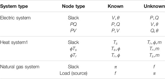
TABLE 1. Different node types with their known and unknown variables.

For electrical networks, $P,Q,V,\text{ and }\theta$ are the active power, reactive power, voltage amplitude, and phase angle of the power system nodes, respectively. In the natural gas network, $f\text{ and }\pi$ are the natural gas injection flow and pressure of the nodes, respectively. $T_s,T_r,\varphi ,\text{ and }m$ are the supply temperature, reflux temperature, heat power, and water flow of the heat source or heat load of the thermal system, respectively.

Heating Network

The steady-state power flow calculation model of the heating network is divided into two parts: hydraulic model and thermodynamic model (Liu, 2013).

Hydraulic Model

The flow of hot water in the network should meet the fundamental law of the network: the flow of each pipeline should satisfy the flow continuity equation at each node, that is, the injection flow at the node is equal to the outflow; in a closed-loop composed of pipes, the sum of the head loss of water flowing in each pipeline is 0, that is,

$\{\begin{array}{l}{A}_{s}m=m_q\\ B_h{h}_f=0\end{array},(1)$

where $A_s$ is the node-branch correlation matrix of the heating network, $m$ is the flow of each pipeline, $m_q$ is the flow out of each node, $B_h$ is the loop-branch correlation matrix of the heating network, $h_f$ is the head loss vector, and its calculation method is as follows:

$h_f=Km\left|m\right|,(2)$

where $K$ is the resistance coefficient matrix of the pipeline.

Thermodynamic Model

For each heat load node, the heating temperature $T_s$ represents the temperature before the hot water is injected into the load node, the output temperature $T_o$ represents the temperature when the hot water flows out of the load node, and the heat recovery temperature $T_r$ represents the temperature after the hot water from the load node is mixed with the water of other pipes at the pipe node.

The thermodynamic model is as follows:

$\Phi =C_p{m}_q\left(T_s-T_o\right),(3)$

$T_{end}=(T_{start}-T_a)e^{-\frac{\lambda L}{C_{p}m}}+T_a,(4)$

$({\displaystyle \sum m_{out}})T_{out}={\displaystyle \sum m_{in}{T}_{in}}.(5)$

Equation 3 is the expression of the node thermal power $\Phi$ of the thermal network, and $C_p$ is the specific heat capacity of water; Eq. 4 represents the relationship between the temperature at the end of the pipe $T_{end}$ and the temperature $T_{start}$ at the beginning, $T_a$ is the ambient temperature, $\lambda$ is the heat conduction coefficient of the pipe, and $L$ is the length of the pipe; Eq. 5 represents the temperature relationship before and after the hot water is mixed at the node, and $m_{out},T_{out}$, $m_{in},T_{in}$ represent the flow rate and temperature of the water flowing out and into the pipe, respectively.

Natural Gas Network

A natural gas system can be specified by several equations related to various elements of this system, including pipelines, compressors, sources, and loads. The input–output flow balance of each node should be considered for a feasible operational condition. The amount of gas flow through a pipeline connected between nodes $i$ and $j$ in standard cubic meter per hour (SCM/h) can be expressed by (De Wolf and Smeers, 2000) the following:

$f_{ij}=C_{ij}sign\left({\pi }_i,{\pi }_j\right){\left[sign\left({\pi }_i,{\pi }_j\right)\ast \left({\pi }_i^2-{\pi }_j^2\right)\right]}^{0.5},(6)$

$C_{ij}=96.074830\times {10}^{-15}\frac{D_{ij}}{{\lambda }_{ij}zT{L}_{ij}\delta },(7)$

${\lambda }_{ij}={\left[2\log \left(\frac{3.7D_{ij}}{{\epsilon }_g}\right)\right]}^{-2},(8)$

where ${\pi }_i$ and ${\pi }_j$ are pressures at the nodes $i$ and $j$, respectively. $sign({\pi }_i,{\pi }_j)$ is a sign function of pressures where its value is $+1$ if ${\pi }_i>{\pi }_j$ and $-1$ otherwise. The pipeline constant can be computed by Eq. 7, where $z$ is the gas compressibility factor, $T$ is the gas temperature, and $\delta$ is the density of gas relative to air. $D_{ij}$ and $L_{ij}$ are the interior diameter and length of the pipeline, respectively. ${\lambda }_{ij}$ is the friction factor of the gas pipeline. It is computed by Eq. 8, where ${\epsilon }_g$ is absolute rigidity of the pipe.

The node flow balance equation of the natural gas network is as follows:

$\Delta f=f_l-f_s+{\displaystyle \sum f_{ij}},(9)$

where $f_l$ is the natural gas flow consumed by the natural gas load, including gas turbine, gas boiler, CHP, and conventional natural gas load. For the compressor inlet node, it should also include the compressor outlet flow, that is, the compressor outlet flow as the load of the inlet node, $f_s$ is the injection flow of the gas source, and ${\displaystyle \sum f_{ij}}$ is the flow of all non-compressor branches connected with the node.

Electric Network

The power system model adopts the AC system model, and the electric load of the heating system and the natural gas system is taken into account. The balance equation of active power and reactive power is as follows:

$\Delta P=P^G-P^l-\mathrm{Re}\left\{U{\left(YU\right)}^{\ast }\right\},(10)$

$\Delta Q=Q^G-Q^l-\mathrm{Im}\left\{U{\left(YU\right)}^{\ast }\right\},(11)$

where $P^G\text{ and }{Q}^G$ are the active power and reactive power generated by the generator, respectively; $P^l\text{ and }{Q}^l$ are the active power and reactive power consumed by the load in the electric network, respectively.

Coupling Units

The coupling units of electricity, gas, and heat integrated energy systems mainly include CHP, gas boiler, gas turbine, electric compressor, and water pump.

CHP is the main coupling unit in electric, gas, and thermal systems. CHP is a kind of unit which not only generates electricity by a steam turbine but also supplies heat to thermal users by steam after power generation. The ratio of heat generation power to electricity generation power of CHP with gas turbine and reciprocating internal combustion engine in prime mover can be regarded as a constant, and the ratio of heat to electricity can be expressed as follows:

$c_m={\varphi }_{CHP}/P_{CHP},(12)$

where $P_{CHP}\text{ and }{\varphi }_{CHP}$ are the power generated and thermal power of CHP, respectively, and $c_m$ is the thermoelectric ratio of CHP.

According to the working mode, CHP can be divided into back pressure type and pumping type. The heat-power ratio of the back pressure CHP unit is constant, while the extraction–condensation CHP unit changes the heat-power ratio of the CHP unit by adjusting the amount of steam extracted, and its output is mainly related to the natural gas flow consumed, that is,

$f_{CHP}=\frac{P_{CHP}}{q_{gas}{\eta }_e}+\frac{{\varphi }_{CHP}}{q_{gas}{\eta }_h},(13)$

where $f_{CHP}$ is the natural gas flow consumed by CHP and $q_{gas}$ is the calorific value of natural gas. ${\eta }_e$ and ${\eta }_h$ represent the power generation efficiency and heat generation efficiency of CHP, respectively.

The gas turbine is the equipment that consumes natural gas to generate electric energy. The relationship models between the consumed natural gas flow and the generated power are as follows:

$f_G=a_G+b_G{\varphi }_G+c_G{\varphi }_G^2,(14)$

where $f_G$ is the natural gas flow consumed by the gas turbine, $P_G$ is the electric power generated by the gas turbine, and $a_G,b_G,\text{ and }{c}_G$ are consumption coefficients of the gas turbine.

MEF Model

Based on the above, an IES-oriented MEF model is constructed as follows:

$F\left(x\right)=\left\{\begin{array}{l}△P\\ △Q\\ △\Phi \\ △p\\ △T_s\\ △T_r\\ △f\end{array}\right\}=\{\begin{array}{l}\Delta P=P^G-P^L-\mathrm{Re}\left\{U{\left(YU\right)}^{\ast }\right\}\\ \Delta Q=Q^G-Q^L-\mathrm{Im}\left\{U{\left(YU\right)}^{\ast }\right\}\\ C_p{A}_{s}m\left(T_s-T_o\right)-\Phi =0\\ B_{h}Km\left|m\right|=0\\ C_s{T}_{s,load}-b_s=0\\ C_r{T}_{r,load}-b_r=0\\ f_l-f_s+{\displaystyle \sum f_{ij}=0}\end{array}.(15)$

In Eq. 15, the first row and the second row represent the active power deviation and reactive power deviation of the power system, respectively. The third to the sixth lines represent the node thermal power deviation of the thermal system, the pressure drop deviation of the heating network loop, the heating temperature deviation, and the regenerative temperature deviation, respectively. The seventh line represents the node flow deviation of the natural gas system. $P^G$, $Q^G$, $\Phi$, and $f_l$ are the active power, reactive power, thermal power, and natural gas load given by the system, respectively. $P^L$ and $Q^L$ are the total active load and reactive load, respectively. $A_s$ is the incidence matrixes of the heating network. $C_s$ and $C_r$ are matrices related to the structure and flow of heating network and regenerative network, respectively, while $b_s$ and $b_r$ are column vectors related to heating temperature and output temperature, respectively.

It is worth noting that the power balance equation of power network includes trigonometric function, the flow balance equation of gas network involves non-convex nonlinear pipeline flow equation, and the heat network temperature balance equation includes exponential equation so that the IES-oriented MEF model is a non-convex nonlinear problem, which makes it difficult for us to solve MEF directly with traditional methods, and the calculation accuracy is difficult to be guaranteed.

Therefore, in this article, the convex optimization of the non-convex nonlinear equations will be carried out below, which can not only ensure accuracy but also greatly simplify the calculation process and shorten the calculation time.

Calculation Method of Multi-Energy Flow in Integrated Energy Systems

Electric Network

Rectangular Formulation

Let $Y$ denote the nodal admittance matrix, which has components $Y_{ij}=G_{ij}+i{B}_{ij}$ for each line. The complex voltage (also called voltage phasor) $V_i$ at bus $i$ can be expressed in the rectangular form as $V_i=e_i+i{f}_i$.

With the above notation, the power flow conservation at each bus is given in the so-called rectangular formulation as follows:

$P_i^G-P_i^l=G_{ii}\left(e_i^2+f_i^2\right)+{\displaystyle \sum _{j\in \delta \left(i\right)}{G}_{ij}}\left(e_i{e}_j+f_i{f}_j\right)-{\displaystyle \sum _{j\in \delta \left(i\right)}{B}_{ij}}\left(e_i{f}_j-f_i{e}_j\right),(16)$

$Q_i^G-Q_i^l=-B_{ii}\left(e_i^2+f_i^2\right)+{\displaystyle \sum _{j\in \delta \left(i\right)}{B}_{ij}}\left(e_i{e}_j+f_i{f}_j\right)-{\displaystyle \sum _{j\in \delta \left(i\right)}{G}_{ij}}\left(e_i{f}_j-f_i{e}_j\right).(17)$

Generation and voltage bounds at each bus are as follows:

${\left(V_i^{\min }\right)}^2\le e_i^2+f_i^2\le {\left(V_i^{\max }\right)}^2.(18)$

$P_i^{\max }\le P_i^G\le P_i^{\max },(19)$

$Q_i^{\max }\le Q_i^G\le Q_i^{\max }.(20)$

Here, $P_i^l,Q_i^l$ is the summary of all kinds of active and reactive load in the electric system.

Second-Order Cone Program Relaxation of Alternative Formulation

Note that the rectangular formulation of AC power flow is a non-convex quadratic optimization problem. However, quite importantly, we can observe that all the nonlinearity and non-convexity come from one of the following three forms: (1) $e_i^2+f_i^2={\left|V_i\right|}^2$, (2) $e_i{e}_j+f_i{f}_j=\left|V_i\right|\left|V_j\right|\cos ({\theta }_i-{\theta }_j)$, and (3) $e_i{f}_j-f_i{e}_j=-\left|V_i\right|\left|V_j\right|\sin ({\theta }_i-{\theta }_j)$. To capture this nonlinearity, we define new variables $C,S$ to get rid of the variable $e$ and variable $f$ (Kocuk et al., 2016). The new variables are defined as follows:

$C_{ii}=e_i^2+f_i^2,(21)$

$C_{ij}=e_i{e}_j+f_i{f}_j,(22)$

$S_{ij}=e_i{f}_j-e_j{f}_i.(23)$

With a change of variables, we can introduce an alternative formulation of the power flow problem in the electric system as follows:

$P_i^G-P_i^l=G_{ii}\left(C_{ii}\right)+{\displaystyle \sum _{j\in \delta \left(i\right)}{G}_{ij}\left(C_{ij}\right)}-{\displaystyle \sum _{j\in \delta \left(i\right)}{B}_{ij}}\left(S_{ij}\right),(24)$

$Q_i^G-Q_i^l=-B_{ii}\left(C_{ii}\right)-{\displaystyle \sum _{j\in \delta \left(i\right)}{B}_{ij}\left(C_{ij}\right)}-{\displaystyle \sum _{j\in \delta \left(i\right)}{G}_{ij}}\left(S_{ij}\right),(25)$

${\left(V_i^{\min }\right)}^2\le C_{ii}\le {\left(V_i^{\max }\right)}^2,(26)$

$C_{ij}^2+S_{ij}^2=C_{ii}{C}_{jj},(27)$

$C_{ij}=C_{ji},(28)$

$S_{ij}=-S_{ji}.(29)$

Through the above transformation, we convex the original Cartesian coordinate Eqs 16–20 into Eqs 24–29, which is more convenient to solve.

Natural Gas Network

The original Weymouth equation, which represents the relationship between the natural gas flow with the pressure at the inlet and the outlet of a natural gas pipeline, is a non-convex and nonlinear problem and hard to solve directly. Two approximation methods are used to linearize the Weymouth equation.

Method ①: One-dimensional approximation.

From Eq. 6, it can be found that the right side of Eq. 6 is a function of ${\pi }_i^2$ and ${\pi }_j^2$. By introducing variables ${\phi }_i={\pi }_i^2$ and ${\phi }_j={\pi }_j^2$, Eq. 6 can be replaced with (Zhou, 2020) the following:

$f_{ij}=\mathrm{sgn}\left({\phi }_{ij}\right)C_{ij}\sqrt{\left|{\phi }_{ij}\right|},(30)$

${\phi }_{ij}={\phi }_i-{\phi }_j.(31)$

In addition, the node pressure constraint can also be replaced with the following:

${\left({\pi }_i^{\min }\right)}^2\le {\phi }_i\le {\left({\pi }_i^{\max }\right)}^2,(32)$

${\left({\pi }_j^{\min }\right)}^2\le {\phi }_j\le {\left({\pi }_j^{\max }\right)}^2.(33)$

It can be seen that constraint Eq. 30 is a one-dimensional nonlinear equation, which greatly simplifies the linearization process. The upper and lower limits of ${\phi }_{ij}$ can be determined by the following formula:

${\phi }_{ij}^{\max }={\left({\pi }_i^{\max }\right)}^2-{\left({\pi }_j^{\min }\right)}^2,(34)$

${\phi }_{ij}^{\min }={\left({\pi }_i^{\min }\right)}^2-{\left({\pi }_j^{\max }\right)}^2.(35)$

The range $\left[{\phi }_{ij}^{\min },{\phi }_{ij}^{\max }\right]$${\phi }_{ij}$ can be divided into $N_{ij}$ segments, and the nonlinear Eq. 30 can be transformed into Eqs. 36–39:

$\begin{array}{l}{\phi }_{ij}={\phi }_{ij0}+{\displaystyle \sum _{p=1}^{N_{ij}}{\sigma }_{ij,p}}.\\ \end{array}(36)$

$f_{ij}=f_{ij0}+{\displaystyle \sum _{p=1}^{N_{ij}}{K}_p^{ij}}{\sigma }_{ij,p},(37)$

$z_{ij,p+1}\cdot \left(\overline{{\phi }_{ij,p}}-\underset{¯}{{\phi }_{ij,p}}\right)\le {\sigma }_{ij,p},(38)$

${\sigma }_{ij,p}\le z_{ij,p}\cdot \left(\overline{{\phi }_{ij,p}}-\underset{¯}{{\phi }_{ij,p}}\right),(39)$

where $p$ is the one-dimensional piecewise linear segment number index, $z_{ij,p}$ is the binary variable used in the one-dimensional linear approximation method, and $K_p^{ij}$ is the constant of the one-dimensional linear equation.

Method ②: Taylor expansion approximation.

We linearize Eq. 6 by Taylor expansion (Manshadi and Khodayar, 2015) as follows:

$f_{ij}=C_{ij}\left({\pi }_i{\pi }_i^0-{\pi }_j{\pi }_j^0\right)/\sqrt{\left|{\left({\pi }_i^0\right)}^2-{\left({\pi }_j^0\right)}^2\right|},(40)$

where ${\pi }_i^0$ is the initial pressure value of the node $i$ at the beginning of the optimization period and is a known quantity.

The linearization using the Taylor series is valid only if the difference in natural gas pressure between the inlet and outlet of the pipeline is assumed to be limited, that is, there is no significant pressure drop in the pipeline.

This is a reasonable assumption for the short pipelines used in microgrids. The limitation on the node pressure on the gas pipeline network guarantees the accuracy of the approximation. The Weymouth equation is linearized around the initial point procured by solving optimal energy flow within the microgrid considering no disruptions.

By Method ①, we replace the non-convex and nonlinear pipeline Eqs 6–9 with the linear model consisting of Eqs 36–39. By Method ②, we transform the original Weymouth Eq. 6 into the linear model of Eq. 40. Both of them are mature methods and help to solve the problem quickly.

Heating Network

The heating network model studied in this article is the radiant heat network model. The original heating network power flow in Eqs 1–5 is a nonlinear equation. The coupling relationship between temperature and flow is strong and contains an exponential equation, making the computational complexity high so that the numerical stability is difficult to be guaranteed.

Therefore, this study adopts the method (Sun et al., 2020) based on Taylor’s second-order expansion; the specific contents are as follows:

To get the flow $m_i$ of the pipe $i$ in Figure 1, we define $n_1=m_1/m_i$, $n_2=m_2/m_i$∙∙∙$n_{i-1}=m_{i-1}/m_i,n_i=1$; thus,

$\begin{array}{l}\frac{T_s-T_o}{T_s-T_a}{m}_i^2-[\frac{\frac{{\lambda }_1{L}_1}{n_1}+\frac{{\lambda }_2{L}_2}{n_2}+\cdots +\frac{{\lambda }_i{L}_i}{n_i}}{C_p}+\frac{{\varphi }_i}{C_p\left(T_s-T_a\right)}]\times m_i+\frac{{\left(\frac{{\lambda }_1{L}_1}{n_1}+\frac{{\lambda }_2{L}_2}{n_2}+\cdots +\frac{{\lambda }_i{L}_i}{n_i}\right)}^2}{2C_P^2}=0.\\ \end{array}(41)$

FIGURE 1

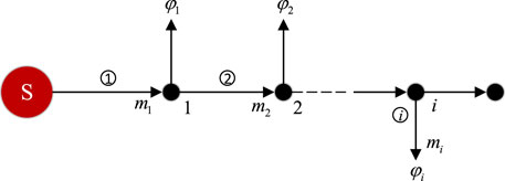
FIGURE 1. A radial district heating network of multiple nodes.

When calculating $n_1{n}_2$,∙∙∙,$n_{i-1}$, the heat loss of the pipe network is ignored, and the heat energy flowing through the pipe $i$ is set to ${\phi }_i$. While to figure the pipe flow $m_i$ into the load node, we set $n_1\approx \frac{C_p{m}_1{T}_1}{C_p{m}_i{T}_i}=\frac{{\phi }_1}{{\phi }_i}$, $n_2\approx \frac{C_p{m}_2{T}_2}{C_p{m}_i{T}_i}=\frac{{\phi }_2}{{\phi }_i}$ ∙∙∙ $n_k\approx \frac{C_p{m}_k{T}_k}{C_p{m}_i{T}_i}=\frac{{\phi }_k}{{\phi }_i}$ as the temperature change of the water supply network node is small. $k$ is the number of the pipe through which the flow $m_i$ flows and ${\phi }_k$ is the heat energy flowing through the pipe $k$. Thus, we can define

$\begin{array}{l}A=\frac{T_s-T_o}{T_s-T_a};C=\frac{{\left(\frac{{\lambda }_1{L}_1}{n_1}+\frac{{\lambda }_2{L}_2}{n_2}+\cdots +\frac{{\lambda }_i{L}_i}{n_i}\right)}^2}{2C_P^2},\\ \end{array}$

$B=-\left(\frac{\frac{{\lambda }_1{L}_1}{n_1}+\frac{{\lambda }_2{L}_2}{n_2}+\cdots +\frac{{\lambda }_i{L}_i}{n_i}}{C_p}+\frac{{\varphi }_i}{C_p\left(T_s-T_a\right)}\right)$

Then the Eq. 42 can be simplified as follows:

$A{m}_i^2+B{m}_i+C=0.(42)$

The value of $C$ is generally less than ${10}^{-4}$ orders of magnitude, then formula (42) can be approximated to

$A{m}_i+B=0.(43)$

In this article, we define Eqs 42, Eqs 43 as model 2 and model 1, respectively.

The flow rate of each pipeline flowing into the load node can be calculated directly by Eq. 42 or Eq. 43, and the supply temperature, return temperature, and pipe flow rate of each node of the heating network can be obtained according to Eqs 1, 3–5.

Model 1 and model 2 decouple the water supply network and the backwater network, decouple the temperature and flow, the model is simple, the amount of calculation is small, and the derivation is based on Taylor’s second-order expansion, and the solution accuracy is higher.

Through the above transformations and simplifications, the original MINLP (mixed-integer nonlinear programming) is reduced to a MICP (mixed-integer convex programming) problem, which can be effectively solved by commercial solvers.

Case Studies and Analysis

Case Introduction

In the example of the integrated energy system used in this article, the power system is an IEEE standard 14-bus system (Kersting, 1991), as shown in Figure 2, in which the generator node is replaced by CHP. In order to match the capacity and power of CHP, the load is increased to 3.6 times, and the active load with a certain capacity is arranged at the balance node. The natural gas system is a 6-node system, and its line parameters refer to the study by Cong Liu et al. (2009). The thermal system adopts the 23-node system in the reference Sun et al. (2020). The topological structure of each system is shown in Figures 2–4. In this article, the FMINCON solver is used to calculate the multi-energy flow in the MATLAB platform.

FIGURE 2

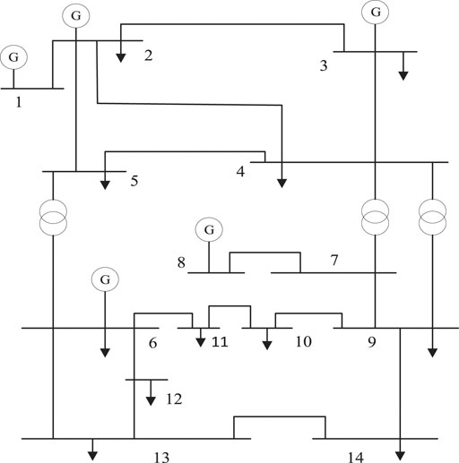
FIGURE 2. IEEE standard 14 bus system.

FIGURE 3

FIGURE 3. Topological structure of the gas network.

FIGURE 4

FIGURE 4. Topological structure of the heating network.

The coupling units between the power grid and the heating network mainly include the CHP units of each coupling node and the coupling unit of the power grid, the gas network includes the CHP of each coupling node and the gas turbine, and the coupling unit between the heat network and the gas network mainly includes the CHP of each coupling node. The connecting nodes and types of coupling units in each network are shown in Table 2.

TABLE 2

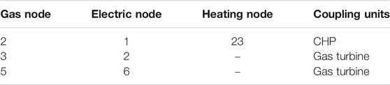
TABLE 2. Connecting nodes and types of coupling units.

In the model of gas turbine, the model parameters of $a_G=c_G=0,b_G=167.1m^3/MWh$. In the model of CHP, this article considers two models: Model I is the pumping type, and Model II is the backpressure type. The parameters of CHP units are shown in Table 3.

TABLE 3

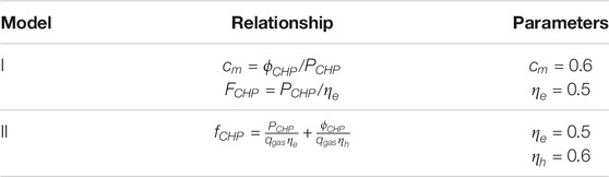
TABLE 3. Parameters of CHP.

Results and Analysis

In this study, we use two models to calculate the mass flow of each pipeline, water supply temperature, and return temperature of each node in the heating network. As is mentioned above, we define Eq. 43 as Model 1 and Eq. 42 as Model 2. Besides, we define Model 3, the control group, as the original model without linearization. The results of the heating network are shown in Tables 4–6.

TABLE 4

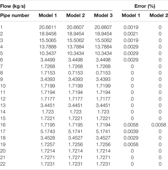
TABLE 4. Mass flow rates of the models.

TABLE 5

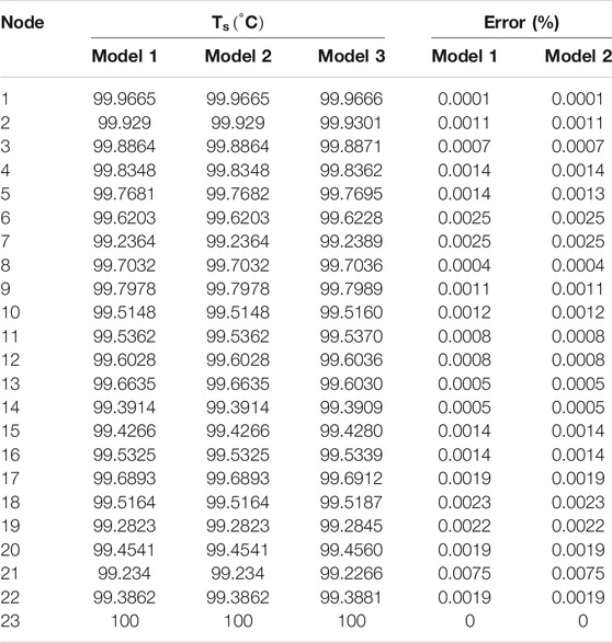
TABLE 5. Water supply temperature and error of the models.

TABLE 6

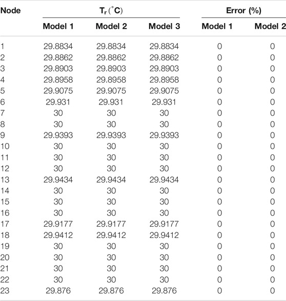
TABLE 6. Water return temperature and error of the models.

In the process of solving, we find that the solving time of mode 1 and mode 2 is millisecond, while that of mode 3 is 21 s. In terms of solving time, the two models have the advantages of small amount of calculations and fast calculation speed.

From the above data, we can see that the maximum error of mass flow in Models 1 and 2 is 0.0058%, the maximum error of water supply temperature is 0.0075%, and return water is the same as that of Model 3. Both Models 1 and 2 have a high precision of solution. While it comes to each pipe's mass flow, Model 2 is more precise because the constant $C$ has influence. Therefore, we use the results of Model 2 for the following calculation.

This study considers two models of CHP units and two linearized methods of the gas network. We define the one-dimensional approximation method in the gas system as Method ① and the Taylor expansion approximation method as Method ②. So there are four running combinations in the following calculation, just as Table 7 shows. The gas network and electric system results are shown in Tables 8–12, including pressure, mass flow, voltage amplitude, and voltage phase angle.

TABLE 7

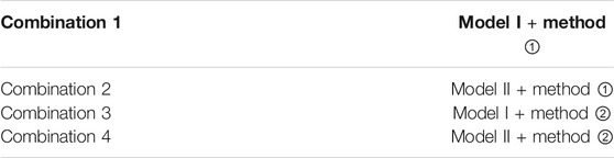
TABLE 7. Four combinations.

TABLE 8

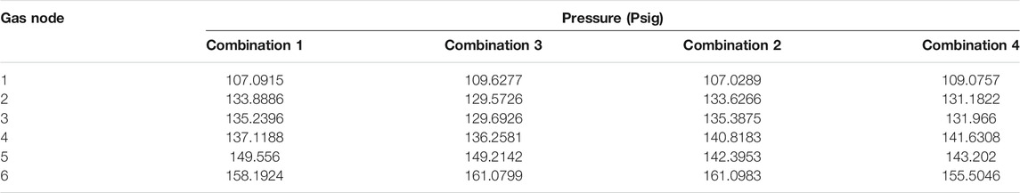
TABLE 8. Pressure of each node in the gas system.

TABLE 9

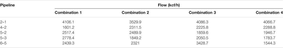
TABLE 9. Mass flow of each pipe in the gas system.

TABLE 10

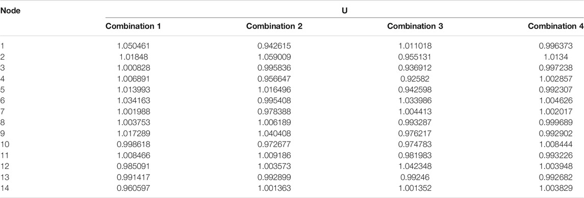
TABLE 10. Voltage amplitude of each node in the electric system.

TABLE 11

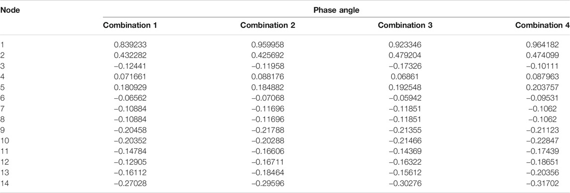
TABLE 11. Voltage phase angle of each node in the electric system.

TABLE 12

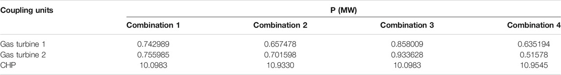
TABLE 12. Power generated by gas turbines and the CHP.

By comparing the results of combinations 1 and 3, and combinations 2 and 4, we can see that no matter which mode the CHP unit runs in, there is a great difference between the results of Methods ① and ②, although the solving speed of both methods is in millisecond. The decisive factors of the accuracy of the two methods are different. Method ① depends on the number of segments and the value of constant $K$, while Method ② is only related to the initial value.

For Method ①, if we want to pursue accuracy, we need to divide more segments to achieve a higher degree of approximation. Still, at the same time, it also increases more unknowns and the amount of calculation, and the operation time becomes longer. Although Method ② is only suitable for networks with short pipeline length, it has a small amount of calculation. It involves fewer unknowns, while the natural gas network pipeline used in this study is shorter, so Method ② is more suitable for this study.

By comparing the results of combinations 1 and 2 and combinations 3 and 4, it can be seen that whichever method solving the gas system is adopted, power generated by the CHP unit is different between the two models. Model II generates more power than Model I, and at the same time, gas turbines generate less power in Model I than in Model II. Besides, when the operation mode of the CHP unit changes, the electric power generated by the CHP unit and the natural gas consumed change, which leads to the change of the power flow distribution of the power grid and the gas network, while in Model I, the electric power generated by the CHP unit depends on the thermal power generated by the CHP unit in the heating network. If the thermal power changes, the power flow distribution of the gas network, and the power grid will also be affected by it.

It can be seen that in the electric/thermal/gas integrated energy system, each network is connected into an inseparable whole through coupling units such as CHP and gas turbine, and the change of network state will affect the trend of other networks through the coupling unit.

Conclusion

To calculate the integrated energy system combined with electricity, gas, and heat more quickly and accurately, a comprehensive multi-energy flow calculation model based on convexification is proposed in this study. The model is established according to the different characteristics of electricity, heat, and gas networks. The natural gas network pipeline model is linearized reasonably, which greatly reduces the complexity of the model. In the heat network, two kinds of radiant heat network models that can be solved quickly are established, and the original model is transformed into the problem of solving univariate first-order equation and univariate quadratic equation, respectively; the amount of calculation of which is small, and the calculation speed is fast without any convergence problem. Considering the backpressure type and the pumping type of CHP, four running combinations combined with two models of CHP and two methods of the gas system have been established. Finally, the simulation results show that the algorithm can complete the convergence quickly, proving the algorithm's rapidity and practicability. In addition, the algorithm used in this study takes into account the interaction between different networks, which can quickly get the distribution of the comprehensive power flow of the system.

Data Availability Statement

The original contributions presented in the study are included in the article/Supplementary Material; further inquiries can be directed to the corresponding author.

Author Contributions

XB provided the overall idea. DC built the model and completed calculation of the article under the guidance of XB.

Conflict of Interest

The authors declare that the research was conducted in the absence of any commercial or financial relationships that could be construed as a potential conflict of interest.

Publisher’s Note

All claims expressed in this article are solely those of the authors and do not necessarily represent those of their affiliated organizations, or those of the publisher, the editors and the reviewers. Any product that may be evaluated in this article, or claim that may be made by its manufacturer, is not guaranteed or endorsed by the publisher.

References

Arnold, M., et al. (2008). First International Conference on Infrastructure Systems & Services: Building Networks for A Brighter Future, 1–6.Distributed Control Applied to Combined Electricity and Natural Gas Infrastructures.

CrossRef Full Text | Google Scholar

Cong Liu, C., Shahidehpourau, M., Yong Fu, fnm., and Zuyi Li, fnm. (2009). Security-constrained Unit Commitment with Natural Gas Transmission Constraints. IEEE Trans. Power Syst. 24(3), 1523–1536. doi:10.1109/tpwrs.2009.2023262

CrossRef Full Text | Google Scholar

Correa-Posada, C. M., and Sanchez-Martin, P. (2015). Integrated Power and Natural Gas Model for Energy Adequacy in Short-Term Operation. IEEE Trans. Power Syst. 30 (6), 3347–3355. doi:10.1109/tpwrs.2014.2372013

CrossRef Full Text | Google Scholar

De Wolf, D., and Smeers, Y. (2000). The Gas Transmission Problem Solved by an Extension of the Simplex Algorithm. Manag. Sci. 46 (11), 1454–1465. doi:10.1287/mnsc.46.11.1454.12087

CrossRef Full Text | Google Scholar

Geidl, M., and Andersson, G. (2007). Optimal Power Flow of Multiple Energy Carriers. IEEE Trans. Power Syst. IEEE 22 (1), 145–155. doi:10.1109/tpwrs.2006.888988

CrossRef Full Text | Google Scholar

Geidl, M. (2007). Integrated Modeling and Optimization of Multi-Carrier Energy Systems. New York: Graz University of Technology.

Gu, Z., Kang, C., Chen, X., Bai, J., Cheng, L., et al. (2015). Operation Optimization of Integrated Power and Heat Energy Systems and the Benefit on Wind Power Accommodation Considering Heating Network Constraints. Proceeding of the CSEE 35 (14), 3596–3604.

Google Scholar

Jia, H., Wang, D., Xu, X., Yu, X., et al. (2015). Research on Some Key Problems Related to Integrated Energy Systems. Automation Electric Power Syst. 38 (7), 198–207.

Google Scholar

Kersting, W. H. (1991). Radial Distribution Test Feeders. IEEE Trans. Power Syst. 6 (3), 975–985. doi:10.1109/59.119237

CrossRef Full Text | Google Scholar

Kocuk, B., Dey, S. S., and Sun, X. A. (2016). Strong SOCP Relaxations for the Optimal Power Flow Problem. Operations Res.

CrossRef Full Text | Google Scholar

Liu, X. (2013). Combined Analysis of Electricity and Heat Networks. Cardiff: Cardiff University.

Manshadi, S. D., and Khodayar, M. E. (2015). Resilient Operation of Multiple Energy Carrier Microgrids. IEEE Trans. Smart Grid. IEEE 6 (5), 2283–2292. doi:10.1109/tsg.2015.2397318

CrossRef Full Text | Google Scholar

Moeini-Aghtaie, M., Abbaspour, A., Fotuhi-Firuzabad, M., and Hajipour, E. (2014). A Decomposed Solution to Multiple-Energy Carriers Optimal Power Flow. IEEE Trans. Power Syst. 29 (2), 707–716. doi:10.1109/tpwrs.2013.2283259

CrossRef Full Text | Google Scholar

OMalley, M., and Kroposki, B. (2013). Energy Comes Together: The Integration of All Systems [Guest Editorial]. IEEE Power Energ. Mag. 11 (5), 18–23. doi:10.1109/mpe.2013.2266594

CrossRef Full Text | Google Scholar

Pan, Z., Guo, Q., and Sun, H. (2016). Interactions of District Electricity and Heating Systems Considering Time-Scale Characteristics Based on Quasi-Steady Multi-Energy Flow. Appl. Energ. 167, 230–243. doi:10.1016/j.apenergy.2015.10.095

CrossRef Full Text | Google Scholar

Shabanpour-Haghighi, A., and Seifi, A. R. (2015). Simultaneous Integrated Optimal Energy Flow of Electricity, Gas, and Heat. Energ. Convers. Manag. 101, 579–591. doi:10.1016/j.enconman.2015.06.002

CrossRef Full Text | Google Scholar

Sun, G., Wang, W., Wu, Y., Hu, W., Jing, J., Wei, Z., et al. (2020). Fast Power Flow Calculation Method for Radiant Electric-thermal Interconnected Integrated Energy System. Proc. Chin. Soc. Electr. Eng. 40 (13), 4131–4142.

Google Scholar

Xu, F., Min, Y., Chen, L., Chen, Q., Hu, W., Zhang, W., et al. (2014). Combined Electricity-Heat Operation System Containing Large Capacity thermal Energy Storage. Proceeding of the CSEE 34 (29), 5063–5072.

Google Scholar

Xu, X., Jin, X., Jia, H., Yu, X., and Li, K. (2015). Hierarchical Management for Integrated Community Energy Systems. Appl. Energ. 160, 231–243. doi:10.1016/j.apenergy.2015.08.134

CrossRef Full Text | Google Scholar

Yang, Y., et al. (2010). Chosen Method of Optimum Cold Source Thermal-system Heater in Heat and Power Cogeneration System. Proc. Chin. Soc. Electr. Eng. 30 (26), 1–6.

Google Scholar

Zhang, Y. (2005). Study on the Methods for Analyzing Combined Gas and Electricity Networks. Beijing: China Electric Power Research Institute.

Zhou, X. (2020). Research on Optimal Scheduling of Gas-Electricity Interconnected Integrated Energy System Based on Piecewise Linearization of Weymouth Equation. Nanjing Normal University.