Optimized Placement of Voltage Sag Monitors Considering Distributed Generation Dominated Grids and Customer Demands

Voltage sag causes serious economic losses to sensitive customers. However, the existing optimal placement methods of sag monitors ignore the economic needs of customers. The optimal placement model of voltage sag monitor is proposed in this paper, which considers the sag economic loss weight, realizes the redundant coverage of important customers, and reduces the risk of sag loss of them. The model is also suitable for the system with a large number of DG access. Firstly, the calculation model of exposed area based on Chebyshev iterative method is established to obtain the system exposed area quickly, and the influence of DG replacing traditional generator on exposed area and economic loss is analyzed qualitatively. Then, the economic loss is quantitatively evaluated based on the exposed area. What’s more, the priority of important customers is determined accordingly, and the optimal placement model of sag monitor is proposed. Finally, simulation results show that in large-scale DG access, the customer’s economic loss caused by sag will increase. Compared with traditional methods, this method can reduce the risk of loss and ensure the economic benefits of important customers.

Introduction

Voltage sag is an event caused by a sudden large current in the system and has become a major threat to the normal and safe operation of electrical equipment in power systems. Relevant US power research institutes indicate that sags cause economic losses to customers as high as 26 billion dollars each year (Chun-Tao and Jian-Tong, 2015). Therefore, customers are paying more attention to voltage sag (Ansal, 2020). Timely and accurate monitoring of sags helps to quickly facilitate control measures, thereby minimizing the risk of customers’ economic losses. However, it is difficult to install monitors at each node in the actual process due to installation cost constraints (Sun et al., 2021). The risk of customers missing sag treatment opportunities is significantly increased when sag sensitive areas are unmonitored due to failure or an insufficient number of monitors. From this point of view, the number of monitors and the risk of customers suffering sag economic losses are conflicting goals. Satisfying the power demand of customers is an important task of power grid companies. Therefore, under the constraint of sag observability, it is of great theoretical value and engineering significance to develop a multi-objective optimal placement model considering the number of monitors and the risk of customer sag economic loss. In addition, the scope of the voltage sag sensitive area is further expanded (Wang et al., 2019; Zhang et al., 2021) due to new energy grid capacity limitations and control characteristics (Fu et al., 2021a; Tian et al., 2021), which correspondingly increase the risk of the above-mentioned missed measurement events for customers. Therefore, in a power grid dominated by distributed power generation (Du et al., 2020; Du et al., 2021), it is essential to consider the economic losses of customers in the optimal placement of monitors.

At present, much work has been done at home and abroad to optimize the placement of sag monitors. The most important research method is the Monitor Reach Area (MRA) method (Olguin et al., 2006). In this method, the sag caused by any short circuit of the line can be recognized by at least one sag monitor as a constraint condition, and the goal is to develop an optimized monitor installation plan with the minimum number of monitors (Espinosa-Juarez et al., 2009). Programming algorithms, such as genetic, particle swarm, and integer linear can be used to solve this problem (Espinosa-Juarez et al., 2009; Almeida and Kagan, 2011; Zhou and Tian, 2014). Unfortunately, in practical applications, the monitoring schemes obtained by applying these models are usually not unique, and it is difficult to select an optimal solution. The placement lacks pertinence because the existing placement process methods default to all nodes in the power system being equally important, ignoring the complexity of the actual operation process of the system. Thus, the optimization conditions are insufficient and it is difficult to find an optimal solution. Subsequent studies helped to determine an optimal placement plan solution by introducing new optimization goals, such as the largest sag observability index (Jiang et al., 2020), largest sag severity index (Ibrahim et al., 2010), largest sag weight coefficient (Šipoš et al., 2021), smallest uncertainty area index (Zhang et al., 2019), and largest immunity index (Luo et al., 2019). These studies can uniquely determine the monitoring plan for sags but mainly focus on the system side and ignore the monitoring demands of sensitive customers. In addition, the number of monitors increase in some of these studies to meet the new optimization goals.

Based on the above analysis, an optimized voltage sag monitor placement model is proposed that simultaneously considers the demands of customers and the power grid and can be used in a power grid dominated by DG. In the first step, an exposed area calculation method based on the Chebyshev iteration is proposed to solve the problem of slow convergence in the exposed area calculation process, which significantly improves the calculation efficiency. Then it is theoretically proved that the replacement of traditional generators by DG will increase the exposed area of the same sensitive node and aggravate the economic losses caused by the failure. In other words, when the total generator output remains unchanged, the severity of voltage sag increases with the increase of DG penetration rate. In the second step, a method to describe a customer’s sag economic loss is proposed based on the concept of the exposed area. According to the sag economic loss, the customer nodes are classified into different important levels. Intuitively, a customer’s monitoring demand for sags is to ensure that the sag can be monitored and managed in real-time to minimize their economic loss. A sag must first be monitored before it can be managed. From this point of view, the monitor should cover areas with serious economic losses. When a sag occurs, the economic loss caused by the omission of the monitor can be avoided. Therefore, in the third step, the objectives are to use the minimum number of monitors to facilitate the maximum coverage of an area with serious economic loss to customers caused by a sag. The observability of sag in the entire network is taken as the constraint to form a multi-objective optimal placement model. The fourth step is to use the IEEE 30-node system to test the proposed model. In the proposed case, the impact of different DG penetration rates on the scope of the exposed area and the customer’s economic loss is analyzed. Additionally, the necessity of considering the customer’s economic loss in the process of optimizing the placement is discussed. The simulation results show that the proposed model has practical application value and can reduce the risk of customers’ sag economic loss while reducing the number of sag monitors and uniquely determining the monitoring plan for sags.

Exposed Area Calculation

The key to the exposed area calculation is to find the critical position where the sag amplitude of the busbar where the sensitive load is located is lower than the set sag threshold when a short-circuit fault occurs in the line. When the fault point moves on a certain line in the system, the sag amplitude at the busbar, where the sensitive load is located, is a unimodal function with a downward opening, approximated to a quadratic function. It is possible to directly use the sag amplitude at the three positions of 0, 0.5, and 1 on the line for quadratic interpolation and form an equation with the sag threshold to solve the critical point (Park and Jang, 2007). In addition, the golden section method was proposed to improve the calculation speed and accuracy of the critical value (Ma et al., 2019). The key process for solving the exposed area is discussed in the following sections.

Calculation of Residual Voltage at Load

A short-circuit of the line in the system is the main reason for a sag of the sensitive load bus. Therefore, to solve the exposed area, it is first necessary to obtain the residual voltage of the load under different short-circuit types. The short-circuit calculation model of the power system is shown in Figure 1.

FIGURE 1

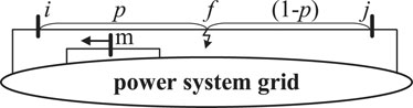
FIGURE 1. Model of power system short-circuit calculation.

We suppose that m is the sensitive bus, the fault is at f in line i-j between nodes i and j, R_f is the fault resistance, and p is the normalized distance from the fault location to node i. First, the power flow calculation is performed and each sequence impedance is formed. Then, the three-phase voltage amplitude of the sensitive bus m is obtained under different fault types and the smallest absolute value is used as the sag amplitude. That is, $\left|V_m^{fault}\right|=\text{min}(\left|V_{A,m}^{fault}\right|,\left|V_{B,m}^{fault}\right|,\left|V_{C,m}^{fault}\right|)$. The calculation formula can be found in (Buzo et al., 2021).

Branch Discriminant Matrix Calculation

After the short-circuit calculation is completed, it is necessary to form discriminant matrices B_sag and L_sag according to the calculation results in subsection A to determine the inclusion of different bus nodes and lines in the sensitive bus-exposed area. First, the sag amplitude vector V_sag of the bus node m is calculated, using:

${\mathit{V}}_{\mathit{sag}}={\left[\begin{array}{ccccc}\left|V_m^{fault\_1}\right|& \cdots & \left|V_m^{fault\_u}\right|& \cdots & \left|V_m^{fault\_n}\right|\end{array}\right]}^{\text{T}}(1)$

where $\left|V_m^{fault\_u}\right|$ denotes the sag amplitude at bus m when bus u fails, and n is the total number of buses in the system. Then, the discriminant matrices B_sag and L_sag are formed to determine the calculation lines required by the Chebyshev iteration method. The element b_sag,u of the B_sag matrix is determined by the difference $\mathit{\Delta }{\mathit{V}}_{\mathit{sag}}$ between the sag amplitude vector V_sag of bus m and the sag threshold vector V_th, expressed as:

$\mathit{\Delta }{\mathit{V}}_{\mathit{sag}}={\left[\Delta v_{sag,1}\cdots \Delta v_{sag,u}\cdots \Delta v_{sag,n}\right]}^{\text{T}}{\mathit{V}}_{\mathit{sag}}\mathrm{-}{\mathit{V}}_{\mathit{th}}(2)$

$b_{sag,u}=\{\begin{array}{l}1\mathrm{;}\text{if}\Delta v_{sag,u}\le \text{0}\\ \text{0}\mathrm{;}\text{if}\Delta v_{sag,u}\text{>0}\end{array}(3)$

If the number of lines is v, the parameter matrix L_sag of the line can be further determined according to the matrix B_sag, expressed as:

${\mathit{L}}_{\mathbf{sag}}=\left[\begin{array}{c}{l}_{sag,1}\\ ⋮\\ l_{sag,v}\end{array}\right]=\left[\begin{array}{c}⋮\\ b_{sag,i}\\ ⋮\end{array}\right]+\left[\begin{array}{c}⋮\\ b_{sag,j}\\ ⋮\end{array}\right](4)$

where i and j represent the node numbers of the busbars at both ends of the corresponding line where they are located. When the element in L_sag is 0, the corresponding line i-j is not in the m-exposed area, and no subsequent calculation is required. When it is 1, the line i-j contains a critical point, and 2 denotes two critical points.

Chebyshev Iterative Method to Calculate Critical Point of the Line

The number of critical points in the line can be obtained through the discriminant matrix in Branch Discriminant Matrix Calculation subsection. Next, on the basis of Branch Discriminant Matrix Calculation Subsection, the specific position of the critical point is solved by curve fitting. When calculating the critical point of the line, the convergence speed of the dichotomy method (Park and Jang, 2007) is the same as the geometric series with a common ratio of 0.5. The golden section method (Ma et al., 2019) has two division points for each contraction interval, 0.618 and 0.382. Thus, in the worst case, the convergence speed is slower than the dichotomy method. To improve the computational efficiency, this study proposes the use of the Chebyshev iteration method with a third-order convergence rate, expressed as:

$x_{k+1}=x_k-\frac{f\left(x_k\right)}{f\prime \left(x_k\right)}-\frac{f″\left(x_k\right){\left[f\left(x_k\right)\right]}^2}{2{\left[f\prime \left(x_k\right)\right]}^3}(5)$

Theoretically, the Chebyshev iteration method has the fastest convergence rate among the three methods. L_sag must first be calculated to determine the critical point in the line. When l_sag,v = 0, line v is outside the exposed area at this time. When l_sag,v = 1, there is only one critical point on the line. First, the sag amplitude $\left|f\left(0.5\right)\right|$ of bus m at position p = 0.5 on the line i-j is calculated, and the sag amplitudes $\left|V_m^{fault\_i}\right|$ and $\left|V_m^{fault\_j}\right|$ of bus m at the end of the fault are combined. The quadratic curve of the sag amplitude changing with the line fault point is fitted and expressed as f (p) = dp² + ep + g, where d, e, and g are constants. Next, the Chebyshev iteration method is used to solve the critical point. The line has two critical points when l_sag,v = 2. To obtain an accurate solution, it is first necessary to solve the fault point $p_{\text{max}}$ that maximizes the m sag amplitude in the line, which is used to preliminarily divide the range of the two solutions, $p_1$ and $p_2$. That is, $0\le p_1<p_{\text{max}}$ and $p_{\text{max}}<p_2\le 1$. Then, the Chebyshev iteration method is used in their respective intervals to solve the exact values of the two critical points. The fitting curve f is a quadratic curve, so its first and second derivatives on (0, 1) exist and are continuous. Therefore, the initial iteration value can be 0.5 and the tangent method iteration formula can be used to quickly obtain the extreme point $p_{\text{max}}$, expressed as:

$x_{k+1}=x_k-\frac{f\prime \left(x_k\right)}{f″\left(x_k\right)}(6)$

The condition for the end of the above iteration is $f^{\text{′}}\left(x_k\right)<\epsilon$, where $\epsilon >0$ represents the calculation accuracy. The extreme point $p_{\text{max}}$ is obtained from the solution and combined with the endpoint value, and the quadratic curve is fitted again. Then, the exact solution can be obtained using the Chebyshev iteration method in the respective intervals of the two solutions. The lines in the system are traversed and the calculation process is repeated to obtain the exposed area of bus node m.

Impact of Distributed Generator (DG) Replacement of Ordinary Generator on the Scope of the Exposed Area

This subsection qualitatively analyzes the impact of replacing the original ordinary generator of the system with DG on the exposed area of load node. Calculation of Residual Voltage at Load, Branch Discriminant Matrix Calculation, and Chebyshev Iterative Method to Calculate Critical Point of the Line Subsections provide quantitative calculation methods for this scene. The original ordinary generator is used as PV node in the system, and the replaced DG is used as PQ node in the system (Fu et al., 2021b). The proportion of DG to the total active capacity of all generators in the system is taken as the proportion of DG. After the short circuit, PQ node’s voltage support capacity is weaker than that of PV node (Kumar et al., 2020a; Kumar et al., 2020b), so the higher the proportion of DG, the lower the sag amplitude of load node and the higher the vulnerability of voltage sag.

In order to study the change of voltage before and after short circuit when PV node is replaced by PQ node with the same active power, it is assumed that the same node in the system switches between PQ and PV. When there is no short circuit in the system, the other nodes outside PQ (PV) node can be equivalent to an impedance Z_s, which is R_s + jX_s. The admittance form of impedance is Y_s = G_s + jB_s. G_s and B_s are their conductance and admittance respectively.

$\{\begin{array}{l}{G}_s=\frac{R_s}{R_s^2+X_s^2}\\ B_s=\frac{X_s}{R_s^2+X_s^2}\end{array}(7)$

For PQ node, the equation is as follows:

$\{\begin{array}{l}{G}_s\left(e_{s1}^2+f_{s1}^2\right)=P_1\\ B_s\left(e_{s1}^2+f_{s1}^2\right)=Q_1\\ e_{s1}^2+f_{s1}^2=\left(P_1+j{Q}_1\right)/Y_s\end{array}(8)$

e_s1 and f_s1 are the real and imaginary parts of voltage U_s1 at PQ node, P₁ and Q₁ are the active and reactive power flowing through PQ node respectively. For PV nodes, the equation is as follows:

$\{\begin{array}{l}{G}_s\left(e_{s2}^2+f_{s2}^2\right)=P_2\\ e_{s2}^2+f_{s2}^2=U_{s2}\\ e_{s2}^2+f_{s2}^2=\left(P_2+j{Q}_2\right)/Y_s\end{array}(9)$

Among them, e_s2 and f_s2 are the real and imaginary parts of the voltage U_s2 at the PV node, P₂ and Q₂ are the active and reactive power flowing through the PV node respectively.

During normal operation, make the two operating states consistent, that is, P₁ = P₂, Q₁ = Q₂, U_s1 = U_s2. When the short-circuit fault occurs, the equivalent impedance Z_s decreases due to the parallel connection of short-circuit impedance. The absolute values of resistance and reactance change are respectively: $\Delta R$_s and $\Delta X$_s. The equivalent conductance and equivalent reactance after short circuit can be obtained by Eq. 7 can be expressed as follows:

$\{\begin{array}{l}{G}_s\prime =\frac{R_s-\Delta R_s}{{\left(R_s-\Delta R_s\right)}^2+{\left(X_s-\Delta X_s\right)}^2}\\ B_s\prime =\frac{X_s-\Delta X_s}{{\left(R_s-\Delta R_s\right)}^2+{\left(X_s-\Delta X_s\right)}^2}\end{array}(10)$

It can be obtained from Eq. 7 and Eq. 10

$\{\begin{array}{l}\Delta G_s=G_s\prime -G_s>0\\ \Delta B_s=B_s\prime -B_s>0\end{array}(11)$

When PQ node is short circuited, it can be concluded from Eq. 8 and Eq. 10 that under constant active power control, the node voltage $U_{s1}^{\prime }$ satisfies the following relation:

$U{\prime }_{s1}^2=\frac{P_1}{\left(G_s+\Delta G_s\right)}=\frac{P_1+j{Q}_1}{\left(G_s+\Delta G_s\right)+j\left(B_s+\Delta B_s\right)}(12)$

① Assuming that the upper limit of reactive power output of PV node after short circuit is greater than the reactive power required by the support voltage, the PV node voltage $U_{s2}^{\prime }$ does not change.

$U{\prime }_{s2}^2=U_{s2}^2=\frac{P_2}{G_s}=\frac{P_1}{G_s}>{U\prime }_{s2}^2(13)$

② Assuming that the upper limit of reactive power output of PV node is lower than the reactive power required by support voltage after short circuit, PV node can provide partial reactive power, reactive power $Q_2^{\prime }$ to the upper limit of reactive power output Q_m (Q_m > Q₁), voltage $U_{s2}^{\prime }$ will be less than U_s2.

${U\prime }_{s2}^2=\frac{P_2+j{Q}_{\text{m}}}{\left(G_s+\Delta G_s\right)+j\left(B_s+\Delta B_s\right)}>{U\prime }_{s2}^2(14)$

It can be concluded from Eq. 13 and Eq. 14: when the original ordinary generator of the system is replaced by DG controlled by constant active power of the same active capacity, the depth of voltage sag will intensify, which will lead to the expansion of exposed area and increase the economic loss of sag, and further clarify the necessity of considering the economic loss of voltage sag in the Grid dominated by distributed generation.

Optimized Placement of Voltage Sag Monitors

Calculation of Customer Sag Economic Loss Based on Exposed Area

The exposed area is a concept for a bus node. In the actual operation of a power system, customers must be distributed on multiple buses and the exposed areas of multiple busbar nodes can be simultaneously calculated. The more severe the overlap of the exposed areas, the more sensitive customers will be affected by the short circuit of the busbar nodes, subsequently causing more serious economic losses. This phenomenon is shown in Figure 2.

FIGURE 2

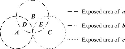
FIGURE 2. Schematic diagram of economic losses caused by short circuits in different areas.

We assume that a, b, and c are three busbars randomly selected from the system and their exposed areas intersect to create five areas, A, B, C, D, and E, as shown in Figure 2. Now a new concept Sag Risk Level (SRL) is introduced to further characterize the sag sensitive area in the system. SRL is corresponding to the redudancy or intersections of exposed areas. For example, the SRL values of areas D and E in Figure 2 are the same. (See Analysis of Customer Sag Economic Loss and Appendix A for details). If the influence of the remaining busbars and lines are temporarily ignored, then the three bus-exposed areas are independently short-circuited and cause their own sags. The economic losses to customers are originally ll_a, ll_b, and ll_c. Subsequently, the economic losses to customers caused by faults in the five areas are ll_a, ll_b, ll_c, ll_a+ ll_b, and ll_b+ ll_c. (See Appendix A for details). From this point of view, the economic losses to customers caused by short circuits in different exposed areas, or even different areas in the same exposed area in the system, are also different. The monitor placement should consider the sag in the entire power grid. This will reduce the risk of economic loss to customers caused by failures in exposed areas that are not monitored in real-time and facilitate corrective measures. Monitoring redundancy should also be improved in the exposed areas that could cause higher economic losses during a fault.

First, to reflect the economic losses caused by independent failures in each busbar exposed area, the vector LE is introduced as:

$\mathit{LE}={\left[\begin{array}{cccc}l{e}_1& l{e}_2& \cdots & l{e}_n\end{array}\right]}^{\text{T}}(15)$

where n represents the number of busbar nodes in the system and the element $l{e}_x,x\in [1,n]$ represents the economic loss to customers when a short circuit occurs independently in the exposed area of node x. The economic loss of customers is obtained through investigation, and the unit of economic loss is yuan. Second, a binary matrix LC is formed according to the calculation result of the exposed area to reflect whether the line is included in the exposed area of the bus, expressed as:

$\mathit{LC}=\left[\begin{array}{cccc}l{c}_{11}& l{c}_{12}& \cdots & l{c}_{1l}\\ l{c}_{21}& l{c}_{22}& \cdots & l{c}_{2l}\\ ⋮& ⋮& l{c}_{cd}& ⋮\\ l{c}_{n1}& l{c}_{n2}& \cdots & l{c}_{nl}\end{array}\right](16)$

where the subscript n represents the number of system nodes, l represents the total number of system lines, and when the system determines, l is also determined. Its element lc_cd obtains a value according to the following formula:

$l{c}_{cd}=\{\begin{array}{l}1\text{; line }d\text{ is in the exposed area of bus }c\\ \text{0; Other situations}\end{array}(17)$

Assuming that the failure probability of each line is equal, the vector LO reflecting a customer’s economic loss caused by a sag can be obtained using:

$\mathit{LO}=\frac{\mathit{LC}·{\left(\mathit{LC}\right)}^{\text{T}}·\mathit{LE}}{l}(18)$

The above formula is the case for a single fault type. The element value of vector LO represents the expected value of economic loss to customers monitored by different nodes. However, the matrix LC is different for different fault types. Finally, to comprehensively consider the four types of faults, the LO needs to be modified as follows:

$\mathit{LO}={\lambda }_1\mathit{L}{\mathit{O}}^1+{\lambda }_2\mathit{L}{\mathit{O}}^2+{\lambda }_3\mathit{L}{\mathit{O}}^3+{\lambda }_4\mathit{L}{\mathit{O}}^4(19)$

where LO¹, LO², LO³, and LO⁴ represent the customer’s economic loss vector for three-phase, single-phase, two-phase, and two-phase grounding short circuits, respectively, and the coefficients ${\lambda }_1,{\lambda }_2,{\lambda }_3,$ and ${\lambda }_4$ represent the respective probability of occurrence of these types of faults.

Monitor Reach Area Matrix Calculation

A sag caused by a short circuit is random, and the key to the placement of the sag monitor is whether it can accurately identify a sag event caused by any short-circuit fault. The observability of the voltage sag of the system can be reflected by the MRA matrix. Assuming that the number of nodes in the system is n and the number of line segments is s, the MRA matrix M^w under any short-circuit fault type can be expressed as:

${\mathit{M}}^w=\left[\begin{array}{cccc}{m}_{11}^w& m_{12}^w& \cdots & m_{1s}^w\\ m_{21}^w& m_{22}^w& \cdots & m_{2s}^w\\ ⋮& ⋮& m_{ab}^w& ⋮\\ m_{n1}^w& m_{n2}^w& \cdots & m_{ns}^w\end{array}\right](20)$

where w represents four types of faults, and its values 0, 1, 2, and 3 represent the three-phase, single-phase grounding, two-phase, and two-phase grounding short circuits, respectively. M^w is a binary matrix, expressed as:

$m_{ab}^w=\{\begin{array}{c}1V_{ab}\le V_{th}\\ 0V_{ab}>V_{th}\end{array}(21)$

where $a=1,2,\cdots n,b=1,2,\cdots s, V_{ab}$ represents the sag amplitude at node b when the line section a is short-circuited, and$V_{th}$ represents the sag threshold set by the sag monitor. When the element m_ab = 1 in the matrix, it means that a short circuit in line segment a will cause node b to sag and will be monitored. Conversely, a value of 0 means that it cannot be monitored. If some nodes can be determined and the union of the monitoring scopes can cover the entire power system, it is not necessary to place monitors at all nodes to observe considerable sags in the entire grid. This is because the rows in the M^w matrix represent the sag monitoring scope of the corresponding node.

Multi-Objective Optimization Placement of Voltage Sag Monitors That Considers the Number of Monitors and Risk of Customer Sag Economic Loss

This section forms an optimal placement model based on the calculation results of sections A and B. Assuming a total of n nodes in the system, the decision vector for configuring the sag monitors can be expressed as:

$\mathit{X}=\left[\begin{array}{cccc}{x}_1& x_2& \cdots & x_n\end{array}\right](22)$

X is a binary vector, and its elements are obtained according to:

$x_i=\{\begin{array}{l}1\text{; if monitor is needed at }i\\ \text{0; if monitor is not needed at }i\end{array}(23)$

where $i=1,2,\cdots n$. The sag in the entire power grid is considered as a constraint. Thus, the basic principle is that the sag caused by any fault can be recorded by at least one monitor, expressed as:

${\displaystyle \sum _{i=1}^n{x}_i{m}_{ij}}\ge 1(24)$

Considering the high cost of monitors in practical applications, the placement of a minimum number of monitors is the first-level goal, expressed as:

$\min \begin{array}{c}\end{array}{f}_1={\displaystyle \sum _{i=1}^n{x}_i}(25)$

The above placement method defaults to all nodes being equally important. In addition, insufficient optimization conditions result in a non-unique placement scheme. For a long time, the primary task of electric power companies was to meet the electricity demand of customers. However, the sag monitor should now be placed with an emphasis on reducing the risk of economic loss for sensitive customers. Using the economic loss vector shown in Eq. 19, the secondary target is ensuring that the monitor covers the maximum scope of the area where the customer’s economic loss is the most serious. This is expressed as:

$\max \begin{array}{c}\end{array}{f}_2={\displaystyle \sum _{i=1}^n{x}_i·l{o}_i}(26)$

To facilitate the solution, it needs to be deformed according to the actual characteristics of the two objective functions. By introducing a priority factor to Eq. 25, the two goals can be transformed into the following equation:

$\min \begin{array}{c}\end{array}f=\alpha {\displaystyle \sum _{i=1}^n{x}_i}-{\displaystyle \sum _{i=1}^n{x}_i}·l{o}_i(27)$

To determine the value of $\alpha$, a sensitivity analysis is performed on Eq. 26. The number of sag monitors is changed by one, expressed as:

$\Delta {\displaystyle \sum _{i=1}^N{x}_i}=1(28)$

Then, the secondary target change amount is expressed as:

$\begin{array}{c}\Delta \end{array}{f}_2=\left(\Delta {\displaystyle \sum _{i=1}^n{x}_i}·l{o}_i\right)\in \left[0,{\displaystyle \sum _{i=1}^{n}l{e}_i}\right](29)$

Therefore, Eq. 27 becomes:

$\begin{array}{c}\Delta \end{array}f=\alpha \Delta {\displaystyle \sum _{i=1}^n{x}_i}-\Delta {\displaystyle \sum _{i=1}^n{x}_i}·l{o}_i=\alpha -\beta ,\beta \in \left[0,{\displaystyle \sum _{i=1}^{n}l{e}_i}\right](30)$

To ensure that the first-level target is satisfied before the second-level target, $\alpha \gg \beta$. That is, $\alpha \gg {\displaystyle \sum }_{i=1}^{n}l{e}_i$ needs to be satisfied. If target two is divided by ${\displaystyle \sum }_{i=1}^{n}l{e}_i$, the optimal placement model can be expressed as:

$\{\begin{array}{l}\min \begin{array}{c}\end{array}f=\alpha \sum _{i=1}^N{x}_i-\frac{\sum _{i=1}^n{x}_i·l{e}_i}{\sum _{i=1}^{n}l{e}_i},\alpha \gg 1\\ \text{s}\text{.t}\text{.}\sum _{i=1}^n{x}_i{m}_{ij}\ge 1\end{array}(31)$

Case Analysis

Calculation Efficiency Analysis of Exposed Area

The IEEE 30-node method was used to verify the feasibility and effectiveness of the proposed method. The system structure was composed of 37 lines connected to 30 bus nodes, similar to the system in (Wang et al., 2021), as shown in Figure 3.

FIGURE 3

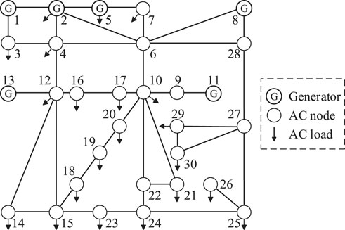
FIGURE 3. Schematic diagram of IEEE 30-node system.

We consider the single-phase grounding short-circuit fault on the line between buses 2 and 4 as an example and calculate its critical point. As l_sag,v = 2, there are two critical points on the line. First, the Chebyshev iteration method is used to calculate the maximum value of the sag amplitude with coordinates $p_{\text{max}}=(0.247,0.8465\text{ p}.\text{u}.)$. This is then combined with the line endpoint coordinates (0.247, 0.813 p. u.) and (0.247, 0.721 p.u.) for quadratic interpolation fitting. The interpolation equation is Uth = -0.6314 p² + 0.4461 p + 0.7746, and the convergence condition was set to ε = 0.0001. The dichotomy (Zhang et al., 2019), golden section (Luo et al., 2019), and Chebyshev methods are used to calculate the critical points. The relationship between the calculation errors of the three methods and the number of iterations is shown in Figure 4.

FIGURE 4

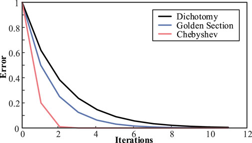
FIGURE 4. Comparison chart of the relationship between error and number of iterations.

When the sag threshold was set to 0.84, the solution critical points were 0.2076 and 0.4989. The dichotomy, golden section, and Chebyshev methods required 11, 9, and 3 iterations to meet the accuracy requirements, respectively, as shown in Figure 5. This shows that the Chebyshev iteration method can reduce the calculation time and occupied resources in practical applications, which is of great significance to the optimization of calculations.

FIGURE 5

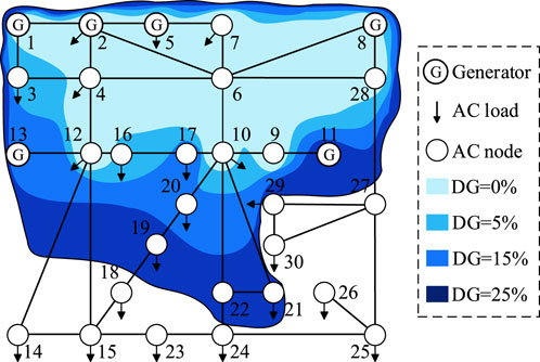
FIGURE 5. Exposed area under different DG penetration rate.

Some cases are now proposed to demonstrate the performance of the proposed optimization model and analyze the scope of the exposed area under different DG penetration levels. The IEEE 30-node test system (a mesh power network) was used and it was assumed that the voltage sags were caused by single-phase short-circuit faults. The considered scenarios of DG penetration are:

Case A1. Base case. The data used is provided from (Wang et al., 2021), which means that there is no DG. The capacities of generators 1, 2, 5, 8, 11, and 13 are 100, 80, 50, 20, 20, and 20 MW, respectively.

Case A2. The DG penetration rate is 5%. The generator at node 11 in Case A1 is replaced with DG with capacity of 20 MW.

Case A3. The DG penetration rate is 15%. The generators at nodes 11, and 13 in Case A1 are replaced with DGs with capacities of 20 and 20 MW, respectively.

Case A4. The DG penetration rate is 25%. The generators at nodes 5 and 11 in Case A1 are replaced with DGs with capacities of 50, and 20 MW, respectively.

In all cases, the DG replaced the generators in the original IEEE 30-node system and used a constant power control method. The exposed area of the node under the four cases were calculated using node 7 as an example, as shown in Figure 5.

Since IEEE 34 node itself is not connected to ordinary generator, some modifications are made to the system in order to analyze the impact of replacing existing ordinary generator with DG on sag. The modified IEEE 34-node system (a radial distributed power network) was used and it was assumed that the voltage sags were caused by single-phase short-circuit faults. The considered scenarios of DG penetration are:

Case A5. Base case. The data used is provided from (Niknam et al., 2003), which means that there is no DG. The active power capacity of generators at nodes 9, 21 and 30 are 90, 120 and 150 kW respectively.

Case A6. The DG penetration rate is 25%. The generator at node 9 in Case A5 is replaced with DG with capacity of 90 kW.

Case A7. The DG penetration rate is 35%. The generator at node 21 in Case A5 is replaced with DG with capacity of 120 kW.

Case A8. The DG penetration rate is 42%. The generator at node 30 in Case A5 is replaced with DG with capacity of 150 kW.

In all cases, the DG replaced the generators in the original IEEE 34-node system and used a constant power control method. The exposed area of the node under the four cases were calculated using node 4 as an example, as shown in Figure 6.

FIGURE 6

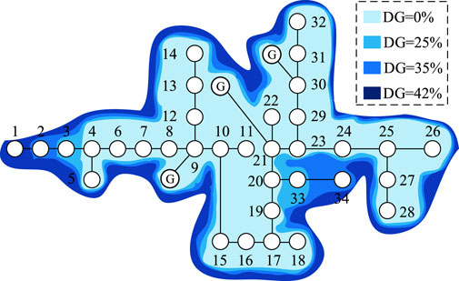
FIGURE 6. Exposed area under different DG penetration rate.

As the penetration rate of DG increased, the scope of the exposed area gradually expanded, as shown in Figure 5 and Figure 6. Additionally, the hazard degree of the sag became more serious and the resulting economic loss was greater. Therefore, it is necessary to consider the customers’ economic losses caused by sags in a grid dominated by DG.

Analysis of Customer Sag Economic Loss

First, the sag threshold was set to 0.9 p. u. Then, the traditional placement model shown in Eq. 24 and Eq. 25 was solved and the placement plan to realize the observability of the voltage sag in the entire power grid was obtained, as shown in Table 1. It can be seen from the table that the scheme meeting the minimum number of monitors is not unique.

TABLE 1

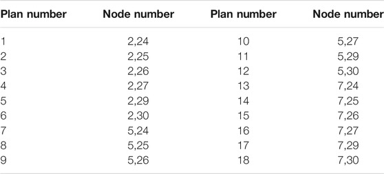
TABLE 1. Placement plan obtained by traditional method.

Field investigations in a certain city were conducted during the process of optimizing the placement of the sag monitor to consider the sag economic loss to different types of customers. The relevant data are shown in Table 2.

TABLE 2

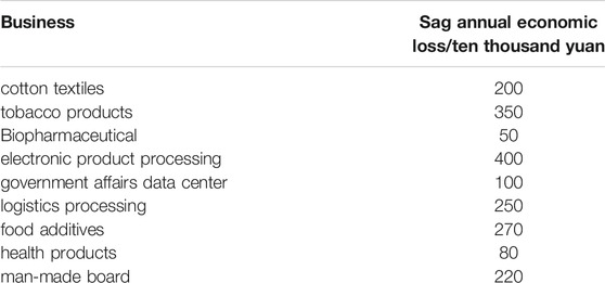
TABLE 2. Customers’ economic losses caused by the sag.

A simulation calculation was carried out in the IEEE 30-node system, and the distribution of various system customers was artificially and randomly assumed. The distribution of different customers in the system is shown as a black solid circle in Figures 6–8, and the sag annual economic loss is marked in bold black font. At this time, we can obtain the vector LE = (0, 0, 400, 250, 0, 270, 350, 0, 0, 200, 0, 0, 0, 100, 0, 80, 0, 0, 0, 50, 0, 0, 0, 0, 0, 0, 0, 220, 0, 0). Then, the calculation results of the exposed area of all buses are used to form the matrix LC and vector LO from Eq. 19. Subsequently, the optimization model shown in Eq. 31 can be used to obtain the optimal placement scheme.

Some additional cases are proposed to consider the influence of DG permeability. The scenarios considered for DG penetration are as follows:

Case B1. Base case. The data used is provided from Ref. (Wang et al., 2021), which means that there is no DG. The capacities of generators 1, 2, 5, 8, 11, and 13 are 100, 80, 50, 20, 20, and 20 MW, respectively.

Case B2. The DG penetration rate is 5%. The generator at node 11 in Case B1 is replaced with DG with capacity of 15 MW.

Case B3. The DG penetration rate is 15%. The generators at nodes 11, and 13 in Case B1 are replaced with DGs with capacities of 25 and 20 MW, respectively.

Case B4. The DG penetration rate is 25%. The generators at nodes 5 and 11 in Case B1 are replaced with DGs with capacities of 50, and 20 MW, respectively.

The monitoring scheme for Case B1 is to place a monitor at nodes 7 and 30. To illustrate the effectiveness of the proposed method, a group of schemes, such as 5 and 26, were randomly selected from the placement schemes obtained by the traditional method for comparison with schemes 7 and 30 that were obtained with the proposed method.

The sag monitoring scope for the proposed method and traditional programs (Zhou and Tian, 2014) are based on the calculation results of the exposed area, as shown in Figure 7.

a) Schematic Diagram of the Monitoring Scope of Traditional Programs.

b) Schematic Diagram of the Monitoring Scope of the Proposed Method.

FIGURE 7

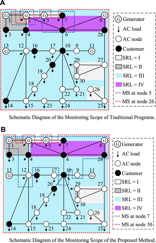
FIGURE 7. Comparison of the monitoring scope of the two schemes.

MS is the abbreviation of monitoring scope, as shown in Figure 7. The MS of the sag monitor at the node refers to the range that can monitor the sag, which is equal to the exposed area under the node setting threshold. The scopes of different monitors are represented by dotted lines of different colors. Lines or nodes with different risk levels are represented by different colored areas according to the following division rules. The total number of occurrences of lines or nodes in all exposed areas can be divided into four intervals representing four different SRL: (0, 7), (Du et al., 2021; Šipoš et al., 2021), (Zhang et al., 2019; Kumar et al., 2020a), and (24, 30). For example, the number of times a line appears in the exposed area of different nodes in the system at the same time is 10, $10\in \left[\mathrm{8,16}\right]$, so the SRL of the line is 2. Only the case of a single-phase short-circuit fault is listed here, but the results under other faults are similar. First, it can be seen from the figure that both monitoring schemes can cover the entire system, indicating that both schemes can achieve the observability of voltage sags in the entire power grid. However, fewer monitors were used by the proposed method. Second, the monitoring program used by the proposed method could simultaneously monitor a wider range of sag sensitive areas. Third, assuming that the failure probability of each line is the same, the X*LC*(LC)^T values of the traditional and proposed schemes can be calculated by rewriting Eq. 18 and Eq. 26, respectively, as:

$\begin{array}{l}[\mathrm{2,5,12,17,4,13,12,5,24,29,1,26,2,29,29,29},\\ \mathrm{29,29,29,29,30,31,32,33,33,33,33,18,33,33}]\end{array}(32)$

$\begin{array}{l}[\mathrm{2,7,20,25,4,21,20,10,31,37,1,33,2,37,37,37},\\ \mathrm{37,37,37,37,38,39,40,41,41},\mathrm{41,41,26,41,41}]\end{array}(33)$

The traditional and proposed schemes monitor and obtain the total economic loss X*LC*(LC)^T *LE/l caused by the sag to customers as 8.97 and 13.12 million yuan, respectively. The results show that the proposed method can effectively improve the monitoring reliability and redundancy in areas that have a serious impact on customer losses when sags occur. Additionally, the proposed method reduces the risk of missing voltage sags due to the failure of a monitor. This facilitates timely governance measures, improves the quality of the power supply to customers, and fundamentally reduces the economic loss of customers.

The monitoring schemes of Cases B2 and B3 are the same, with monitors placed at nodes 7 and 30. In Case B4, only one monitor was installed at node 30. The monitoring scopes for Cases B2 and B3 are shown in Figure 8 and Figure 9, respectively.

FIGURE 8

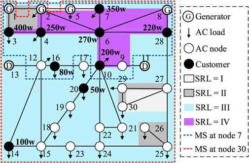
FIGURE 8. Monitoring scope of case B2.

FIGURE 9

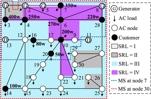
FIGURE 9. Monitoring scope of case B3.

The monitoring scope gradually expands and the sag risk level of the line rises with an increase in DG permeability, as seen in Figures 7–9. The total economic losses to customers caused by the sag are monitored at 14.19 and 15.26 million yuan, as seen in Figures 8, 9, respectively. This again shows that the economic loss caused by the voltage sag in a DG-dominated power grid is more serious. Therefore, to meet the power demand of customers, it is necessary to consider the optimal placement of monitors to reduce the risk of customers’ economic loss. The results show that when the DG penetration rate increases to 25%, the installation of a monitor at node 30 can achieve observability of the sag in the entire system, as shown in Case B4. At this time, the total economic loss to customers caused by the sag is monitored at 8.29 million yuan.

Conclusion

Starting from the primary task of power grid company to meet the power demand of customers, this paper proposes the optimal placement model of sag monitor considering the economic loss of customers, which realizes the redundant coverage of important customers and ensures the economic benefits of them. The main conclusions are as follows:

① The Chebyshev iterative method is used to calculate the exposed area. The Chebyshev iterative method has the advantage of third-order convergence speed, which effectively improves the efficiency of solution. ② The derivation proves that the use of DG to replace the original ordinary generators in the system will result in the expansion of exposed area, thus increasing the economic losses suffered by customers. It verifies the necessity of considering the economic losses of customers in the Grid dominated by distributed generation. ③ Based on the exposed area, a method to calculate the economic loss of customers is proposed. ④ Considering the weight of customer’s economic loss, the optimal placement model of sag monitor is proposed, and the placement scheme with low monitoring cost and high monitoring ability for important customers is obtained, which reduces the risk of customer’s economic loss.

Data Availability Statement

Publicly available datasets were analyzed in this study. This data can be found here: https://pan.baidu.com/s/1tcx_GEVFSJI0uT05RKHggg password:6fda.

Author Contributions

YW contributed to conception and design of the study. QF organized the database. YC performed the statistical analysis. HH wrote the first draft of the manuscript. XX wrote sections of the manuscript. All authors contributed to manuscript revision, read, and approved the submitted version.

Conflict of Interest

The authors declare that the research was conducted in the absence of any commercial or financial relationships that could be construed as a potential conflict of interest.

Publisher’s Note

All claims expressed in this article are solely those of the authors and do not necessarily represent those of their affiliated organizations, or those of the publisher, the editors and the reviewers. Any product that may be evaluated in this article, or claim that may be made by its manufacturer, is not guaranteed or endorsed by the publisher.

References

Almeida, C., and Kagan, N. (2011). Using Genetic Algorithms and Fuzzy Programming to Monitor Voltage Sags and Swells. IEEE Intell. Syst. 26, 46–53. doi:10.1109/mis.2011.2

CrossRef Full Text | Google Scholar

Ansal, V. (2020). ALO-optimized Artificial Neural Network-Controlled Dynamic Voltage Restorer for Compensation of Voltage Issues in Distribution System. Soft Comput. 24, 1171–1184. doi:10.1007/s00500-019-03952-1

CrossRef Full Text | Google Scholar

Buzo, R. F., Barradas, H. M., and Leão, F. B. (2021). A New Method for Fault Location in Distribution Networks Based on Voltage Sag Measurements. IEEE Trans. Power Deliv. 36, 651–662. doi:10.1109/tpwrd.2020.2987892

CrossRef Full Text | Google Scholar

Chun-Tao, M., and Jian-Tong, L. (2015). “Allocation of Voltage Sag Monitoring Based on Improved S-Transform and Exposed Area,” in 2015 Fifth International Conference on Instrumentation and Measurement, Computer, Communication and Control (IMCCC), Qinhuangdao, China, September 18–20, 2015, 1898–1903. doi:10.1109/IMCCC.2015.403

CrossRef Full Text | Google Scholar

Du, W., Wang, Y., Wang, H., Yu, J., and Xiao, X. (2020). Collective Impact of Multiple Doubly Fed Induction Generators with Similar Dynamics on the Oscillation Stability of a Grid-Connected Wind Farm. IEEE Trans. Power Deliv., 1. doi:10.1109/TPWRD.2020.3030645

CrossRef Full Text | Google Scholar

Du, W., Wang, Y., Wang, Y., Wang, H., and Xiao., X. (2021). Analytical Examination of Oscillatory Stability of a Grid-Connected Pmsg Wind Farm Based on the Block Diagram Model. IEEE Trans. Power Syst., 1. doi:10.1109/TPWRS.2021.3077121

CrossRef Full Text | Google Scholar

Espinosa-Juarez, E., Hernandez, A., and Olguin, G. (2009). An Approach Based on Analytical Expressions for Optimal Location of Voltage Sags Monitors. IEEE Trans. Power Deliv. 24, 2034–2042. doi:10.1109/tpwrd.2009.2028777

CrossRef Full Text | Google Scholar

Fu, Q., Du, W., Wang, H. F., and Ren, B. (2021). Analysis of Small-Signal Power Oscillations in MTDC Power Transmission System. IEEE Trans. Power Syst. 36, 3248–3259. doi:10.1109/TPWRS.2020.3043041

CrossRef Full Text | Google Scholar

Fu, Q., Du, W., Wang, H., Ren, B., and Xiao, X. (2021). Small-signal Stability Analysis of a VSC-MTDC System for Investigating Dc Voltage Oscillation. IEEE Trans. Power Syst., 1. doi:10.1109/TPWRS.2021.3072399

CrossRef Full Text | Google Scholar

Ibrahim, A. A., Mohamed, A., and Shareef, H. (2010). “Optimal Placement of Voltage Sag Monitors Based on Monitor Reach Area and Sag Severity index,” in IEEE Student Conference on Research and Development (SCOReD 2010), Kuala Lumpur, Malaysia, December 13–14, 2010. 1, 467–470. doi:10.1109/scored.2010.5704055

CrossRef Full Text | Google Scholar

Jiang, H., Xu, Y., and Liu, Z. (2020). A BPSO-Based Method for Optimal Voltage Sag Monitor Placement Considering Un-certainties of Transition Resistance. IEEE Access 8, 1. doi:10.1109/access.2020.2990634

CrossRef Full Text | Google Scholar

Kumar, N. M., Chopra, S. S., Malvoni, M., Elavarasan, R. M., and Das, N. (2020). Solar Cell Technology Selection for a PV Leaf Based on Energy and Sustainability Indicators-A Case of a Multilayered Solar Photovoltaic Tree. Energies 13, 6439. doi:10.3390/en13236439

CrossRef Full Text | Google Scholar

Kumar, S., Sarita, K., Vardhan, A. S. S., Elavarasan, R. M., Saket, R. K., and Das, N. (2020). Reliability Assessment of Wind-Solar Pv Integrated Distribution System Using Electrical Loss Minimization Technique. Energies 13, 5631. doi:10.3390/en13215631

CrossRef Full Text | Google Scholar

Luo, S. S., Sun, H. T., and Du, X. T. (2019). Research on Optimal Configuration Method of Monitoring Points Considering Sag Positioning and Anti-disturbance Index[J]. Power Capacitors and Reactive Power Compensa-tion 40, 119–125.

Google Scholar

Ma, M., Xu, B. Y., and Wang, Y. (2019). A Hybrid Identifi-Cation Method of Voltage Sag Region Based on Critical point Method. Power Supply and Consumption 36, 50–55.

Google Scholar

Niknam, T., Ranjbar, A. M., and Shirani, A. R. (2003). “Impact of Distributed Generation on volt/Var Control in Distribution Networks,” in 2003 IEEE Bologna Power Tech Conference Proceedings, Bologna, Italy, June 23–26, 2003. 7.

Google Scholar

Olguin, G., Vuinovich, F., and Bollen, M. H. J. (2006). An Optimal Monitoring Program for Obtaining Voltage Sag System Indexes. IEEE Trans. Power Syst. 21, 378–384. doi:10.1109/tpwrs.2005.857837

CrossRef Full Text | Google Scholar

Park, C.-H., and Jang, G. (2007). Stochastic Estimation of Voltage Sags in a Large Meshed Network. IEEE Trans. Power Deliv. 22, 1655–1664. doi:10.1109/tpwrd.2006.886795

CrossRef Full Text | Google Scholar

Šipoš, M., Klaić, Z., and Nyarko, E. K. (2021). Determining the Optimal Location and Number of Voltage Dip Monitoring Devices Using the Binary Bat Algorithm. Energies 14, 255. doi:10.3390/en14010255

CrossRef Full Text | Google Scholar

Sun, R., Ma, J., and Yang, W. (2021). Transient Synchronization Stability Control for Lvrt with Power Angle Estimation. IEEE Trans. Power Electron. 36, 10981–10985. doi:10.1109/tpel.2021.3070380

CrossRef Full Text | Google Scholar

Tian, S. X., Li, K. P., and Wei, S. R. (2021). Distribution Network Security Situation Awareness Method Based on Synchronous Phasor Measuring Device. Proc. Chin. Soc. Electr. Eng. 41, 617–632.

Google Scholar

Wang, Y., Luo, H., and Xiao, X.-Y. (2019). Voltage Sag Frequency Kernel Density Estimation Method Considering protection Characteristics and Fault Distribution. Electric Power Syst. Res. 170, 128–137. doi:10.1016/j.epsr.2019.01.009

CrossRef Full Text | Google Scholar

Wang, Y., Luo, H., and Xiao, X. (2021). Joint Optimal Planning of Distributed Generations and Sensitive Users Considering Voltage Sag. IEEE Trans. Power Deliv., 1. doi:10.1109/tpwrd.2021.3053996

CrossRef Full Text | Google Scholar

Zhang, L., Tong, B., Wang, Z., Tang, W., and Shen, C. (2021). Optimal Configuration of Hybrid AC/DC Distribution Network Considering the Temporal Power Flow Complementarity on Lines. IEEE Trans. Smart Grid, 1. doi:10.1109/TSG.2021.3102615

CrossRef Full Text | Google Scholar

Zhang, Y., Lin, Y. Y., and Shao, Z. G. (2019). Multi-objective Optimal Placement of Positioning Monitoring Points under the Constraints of Considerable Voltage Sag. Trans. Chin. Soc. Electr. Eng. 34, 2375–2383. doi:10.19595/j.cnki.1000-6753.tces.180647

Google Scholar

Zhou, C., and Tian, L. J. (2014). Optimal Configuration of Voltage Sag Monitoring Points Based on Particle Swarm Optimiza-Tion Algorithm. J. Electrotechnical Technol. 29, 181–187. doi:10.19595/j.cnki.1000-6753.tces.2014.04.024

Google Scholar

Appendix A

When a short circuit fault occurs in the intersection of the exposed areas of different load nodes, it will cause the sag of these load nodes at the same time and increase the economic loss of Sag (greater than that of a single load node). The intersection of exposed areas of n ($n\ge 2,n\ge \text{Z}$) load nodes is called redundant area and the redundancy of the redundant area is n. If the sag is not monitored and managed in time, the greater the redundancy is, the greater the economic loss will be suffered by customers, that is, the risk of economic loss will increase with the increase of redundancy. This phenomenon can be explained by Figure 2 in the manuscript. In addition, for the convenience of reviewers, the detailed explanation is as follows:

1) As shown in Figure A1, it is assumed that load node a has x customers, and the exposed area of load node a does not intersect with the exposed area of any other node, that is, the area redundancy represented by the exposed area of load node a is 1.

FIGURE A1

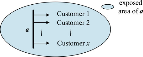
FIGURE A1. Calculation of Economic Loss of Voltage Sag.

Then the total economic loss caused to the customers of node a can be calculated as

${\text{loss}=\text{loss}}_1+{\text{loss}}_2+\dots +{\text{loss}}_o+\dots +{\text{loss}}_x(\mathrm{A1})$

Where loss_o represents the economic loss of the oth ($o\varepsilon [0,x]$) customer.

2) As shown in Figure A2, suppose that load node a has x customers and load node b has y customers, and the exposed area of load node a intersects with that of load node b, the redundancy of the intersection is 2, and the redundancy of the blue and purple areas outside the intersection is 1.

FIGURE A2

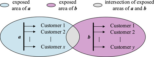
FIGURE A2. Calculation of Economic Loss of Voltage Sag.

When a fault occurs at any position in the intersection, it will cause economic losses to the customers of node a and b. the total loss can be calculated as:

$\begin{array}{c}{\text{loss}=\text{loss}}_1+{\text{loss}}_2+\dots +{\text{loss}}_o+\dots +{\text{loss}}_x\\ +{\text{lloss}}_1+{\text{lloss}}_2+\dots +{\text{lloss}}_p+\dots +{\text{lloss}}_y\end{array}(\mathrm{A2})$

Among them, loss_o represents the economic loss of the oth ($o\varepsilon [0,x]$) customer of node a, and lloss_p represents the economic loss of the pth ($p\varepsilon [0,y]$) customer of node b. The calculation method of the total economic loss caused by the failure in the area with redundancy of 1 is shown in Eq. A1.

3) As shown in Figure A3, assume that load node a has x customers, load node b has y customers, and load node c has z customers, and the exposed areas of load nodes a, b, and c intersect each other. The common intersection of a, b and c is shown in red, and its redundancy is 3, the redundancy of gray area is 2, and the redundancy of other areas is 1.

FIGURE A3

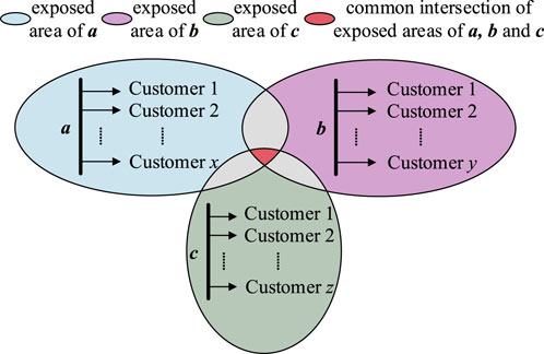
FIGURE A3. Calculation of Economic Loss of Voltage Sag.

When any location in the red area fails, it will cause economic losses to the customers of nodes a, b and c. The total loss can be calculated as:

$\begin{array}{c}{\text{loss}=\text{loss}}_1+{\text{loss}}_2+\dots +{\text{loss}}_o+\dots +{\text{loss}}_x\\ +{\text{lloss}}_1+{\text{lloss}}_2+\dots +{\text{lloss}}_p+\dots +{\text{lloss}}_y\\ +{\text{llloss}}_1+{\text{llloss}}_2+\dots +{\text{llloss}}_q+\dots +{\text{llloss}}_z\end{array}(\mathrm{A3})$

Among them, loss_o represents the economic loss of the oth ($o\varepsilon [0,x]$) customer of node a, lloss_p represents the economic loss of the pth ($p\varepsilon [0,y]$) customer of node b, and llloss_q represents the economic loss of the qth ($q\varepsilon [0,z]$) customer of node c. The calculation method of the total economic loss caused by the failure in the area with redundancy of 1 and 2 respectively is shown in Eq. A1 and Eq. A2. The calculation formula of the sag economic loss increases with the increase of redundancy, and so on.