Classification of Power Quality Disturbance Based on S-Transform and Convolution Neural Network

The accurate classification of power quality disturbance (PQD) signals is of great significance for the establishment of a real-time monitoring system of modern power grids, ensuring the safe and stable operation of the power system and ensuring the electricity safety of users. Traditional power quality disturbance signal classification methods are susceptible to noise interference, feature selection, etc. In order to further improve the accuracy of power quality disturbance signal classification methods, this paper proposes a power quality disturbance classification method based on S-transform and Convolutional Neural Network (CNN). Firstly, S-transform is used to extract disturbance signals to obtain the time-frequency matrix with characteristics of the disturbance signals. As an extension of wavelet transform and Fourier transform, S-transform can avoid the disadvantages of difficult window function selection and fixed window width. At the same time, the feature extracted by S-transform has better noise immunity. Secondly, CNN is used to perform secondary feature extraction on the obtained high-dimensional time-frequency modulus matrix to reduce data dimensions and obtain the main features of the disturbance signal, then the main features extracted are classified by using the SoftMax classifier. Finally, after a series of simulation experiments, the results show that the proposed algorithm can accurately classify single disturbance signals with different signal-to-noise ratios and composite disturbance signals composed of single disturbance signals, and it also has good noise immunity. Compared with other classification methods, the algorithm proposed in this paper has better timeliness and higher accuracy, and it is an efficient and feasible power quality disturbance signal classification method.

Introduction

In modern power systems, the rapid development of renewable energy power generation (Huang et al., 2021; Wang et al., 2021) and related distributed generations and microgrid control strategies (Huang et al., 2019; Wang et al., 2019) have injected a large number of nonlinear signals into the power system. At the same time, there are also a large number of nonlinear loads in the power grid (such as automotive charging piles, power transfer switches). The power grid is showing a power electronic trend, and the power quality problem of the distribution network is becoming more and more serious (Qiu et al., 2020). Frequent occurrences of power quality events cause a lot of economic losses and bring great inconvenience to people’s lives. In order to deal with sudden power quality events, it is necessary to accurately identify and classify the power quality disturbance signals. A convenient, fast and accurate classification algorithm can provide a higher-level application for modern smart meters and real-time monitoring system of power grid (Luo et al., 2018).

Current disturbance signal classification methods mainly include two steps:

1) Extracting characteristics of power quality disturbance signals;

2) Classifying with extracted features.

Feature extraction methods mainly include: Fast Fourier Transform (FFT) (Deng et al., 2020), Wavelet transform (Thirumala et al., 2018), S-transform (Kumar et al., 2015), Hilbert Huang transform (HHT) (Sun et al., 2018), short time Fourier transform (STFT) (Dhoriyani and Kundu, 2020), singular value decomposition (SVD) (Wang et al., 2017), Kalman filter (KF) (Niu et al., 2019). For step 1): due to relatively fixed length and shape of time window, short-time Fourier transform cannot reflect the characteristics of high frequency and low frequency. Although wavelet transform can realize multi-scale focusing, the relationship between transform scale and frequency is fixed. Singular value decomposition and Kalman filter lack the frequency domain characteristics of the signal. S-transform is a reversible time-spectrum positioning technology combining wavelet transform and FFT. It uses an analysis window, the width of the window changes with frequency to provide frequency-related resolution (Kumar et al., 2015). The time-frequency characteristics extracted by S-transform have more significant time-frequency characteristics (Tang et al., 2020).

In comparison, S-transform has higher time resolution and frequency resolution, and is more suitable for analyzing nonlinear, non-stationary, and transient power quality disturbances (Wang et al., 2021a).

The existing classifiers mainly include: artificial neural network (Haddad et al., 2018), Support Vector Machine (SVM) (Yong et al., 2015), decision tree (Huang et al., 2015; Long et al., 2018), expert system (Sai et al., 2015) and Bayesian classifier (Zhou et al., 2011), etc. For step 2): SVM has a high classification accuracy, but the amount of calculation in the process of parameter optimization is relatively large, and the real-time performance is not good. The expert system is a more flexible classification method, but with the increasing of different types of disturbance signals, the complexity of the knowledge base is getting higher and higher, which largely affects the fault tolerance of the system, and the classification performance is also restricted. In view of the problems of existing classifiers, finding a fast and accurate classification method has become the research focus of many researchers.

As the Frontier content in the field of artificial intelligence, neural networks have also made some preliminary applications in the field of power systems, and have achieved some remarkable results. In the field of electricity price forecasting, the literature (Jahangir et al., 2020) has greatly reduced the forecast error. Literature (Jiang et al., 2019) provides an intelligent fault diagnosis method that can automatically identify different health conditions of wind turbine gearboxes. Convolutional neural network (Convolution Neural Network, CNN), as a deep learning method of supervised learning, has advantages of low model complexity and fast calculation speed. Its unique convolution structure can reduce the amount of memory occupied by the deep network and the number of network parameters. CNN has been widely used in face recognition, text recognition and target tracking, as well as semantic segmentation and other fields (Chang et al., 2016; Chowdhury et al., 2016; Chen et al., 2018). In addition, CNN has excellent overfitting treatment methods compared to other classification methods. Methods such as reducing the number of network layers, using Dropout, and adding regular items can be used to improve overfitting.

However, in the field of power quality disturbance classification, the application of CNN is still immature. Only a small amount of literatures use CNN to solve the problem of power quality disturbance signal classification (Chen et al., 2018; Hezuo et al., 2018; Zhu et al., 2019). For example, literature (Chen et al., 2018) uses phase space reconstruction to reconstruct one-bit time series into a multi-dimensional space, then further project the obtained disturbance signal to a two-dimensional phase plane to form a two-dimensional trajectory image, finally input the trajectory image to a CNN for classification. Literature (Hezuo et al., 2018) maps the feature signal into a two-dimensional grayscale image, and then inputs it into a CNN for classification. Literature (Zhu et al., 2019) uses encoding and decoding to extract features of power quality disturbance signals, and then inputs the extracted features into a CNN for classification. However, it is difficult to distinguish the disturbance signal features with high similarity (such as interruption and sag) in the existing methods, and the signal feature extraction process also extracts many features which are irrelevant to disturbance signals. Although the existing methods have high classification accuracy, they still have certain misclassification phenomena.

In view of the above problems, this paper uses the combination of S-transform and CNN to classify power quality disturbance signals. The S-transform is used to extract the characteristic matrix which is used to represent the power quality disturbance signal. According to the three-dimensional (3D) network diagram of each disturbance signal, the sampling range of the feature vector corresponding to the disturbance signal that best represents the disturbance signal is determined. The matrix is trimmed to eliminate the eigenvectors that are useless for specific disturbance signal identification, that is, irrelevant vectors. And then get a square matrix that can represent the characteristics of the disturbance signal and the dimension is $125\times 125$. Input the obtained square matrix into the CNN, and use the CNN to classify the power quality disturbance signal. The combination of S-transform and CNN to classify power quality disturbance signals ensures the efficiency, accuracy and robustness of the classification, and at the same time reduces the misclassification of disturbance signals, which is useful for establishing a real-time monitoring system for modern power grids. It is of great significance to ensure the safe and stable operation of the power system and ensure the safety of users’ electricity.

S-Transform and Feature Extraction

The S-transform proposed by Stockwell (Stockwell et al., 1996) can be regarded as an extension of short-time Fourier transform and wavelet transform, and it is a reversible time-frequency analysis method. S-transform is one of the best techniques for signal processing of non-stationary signals. It uses the phase information of continuous wavelet transform to correct the phase of the original wavelet. It can perform multi-resolution analysis on the signal, just like a set of filters with constant bandwidths. It uniquely has the frequency-related resolution, while positioning the real and imaginary spectra of the phase spectrogram. The time-frequency localization characteristics provided by S-transform are used for subsequent calculations.

Use the FFT and convolution theorem to calculate the S-matrix for each power quality disturbance time. The output of the S-matrix is a complex matrix whose dimension is $k\times n$, and the matrix expression is as follows

$\mathit{S}\left(\mathit{\tau ,f}\right)\mathrm{=}\mathit{A}\left(\mathit{\tau ,f}\right){\mathit{e}}^{-\mathit{i\phi }\left(\mathit{\tau ,f}\right)}(1)$

where $A\left(\tau ,f\right)$ represents amplitude, $\phi \left(\tau ,f\right)$ represents the phase.

The rows of the S matrix represent frequency, and the columns represent time. Each column represents the frequency component that appears in the signal at a specific time, and each row represents a specific frequency signal that occurs at the time from 0 to N−1 on each sampling point. The specific calculation method of S-transform is as follows.

Continuous S-Transform

The continuous S-transformation of the signal h(t) is

$\mathit{S}\left(\mathit{t,f}\right)\mathit{=}{\displaystyle \underset{-\infty }{\overset{+\infty }{\int }}\mathit{h}\left(\mathit{t}\right)\mathit{w}\left(\mathit{t}-\mathit{\tau ,f}\right){\mathit{e}}^{-\mathit{j2\pi f\tau }}\mathit{d\tau }}(2)$

where w is the Gaussian window function, expressed as

$\mathit{w}\left(\mathit{t}-\mathit{\tau }\right)\mathit{=}\frac{\left|\mathit{f}\right|}{\sqrt{\mathit{2\pi }}}{\mathit{e}}^{\frac{-{\left(\mathit{t}-\mathit{\tau }\right)}^{\mathit{2}}{\mathit{f}}^{\mathit{2}}}{\mathit{2}}}(3)$

Discrete S-Transform

The power quality disturbance signal h(t) can be discretized as h(kT), T is the sampling interval; the Fourier transform form of the discrete sampling signal is

$\mathit{H}\left[\frac{\mathit{n}}{\mathit{NT}}\right]\mathit{=}\frac{1}{\mathit{N}}{\displaystyle \sum }_{\mathit{k}=0}^{\mathit{N}-1}\mathit{h}\left(\mathit{kT}\right){\mathit{e}}^{\frac{-\mathit{i2\pi nk}}{\mathit{N}}}(4)$

where $\mathit{n}=\mathrm{0,1},\cdots \mathit{N}-1$.

Let $\mathit{\tau }\to \mathit{jt}$,$\mathit{f}\to \frac{\mathit{n}}{\left(\mathit{NT}\right)}$, the improved discrete S-transform expression is as follows

$\{\begin{array}{c}S\left[\mathit{jT},\frac{\mathit{n}}{\mathit{NT}}\right]={\displaystyle \sum }_{\mathit{m}=0}^{\mathit{N}-1}\mathit{H}\left[\frac{m+n}{\mathit{NT}}\right]\mathit{G}\left(\mathit{m,n}\right){\mathit{e}}^{\frac{\mathit{i2\pi mk}}{\mathit{N}}},n\ne 0\\ S\left[\mathit{jT},0\right]=\frac{1}{\mathit{N}}{\displaystyle \sum }_{\mathit{m}=0}^{\mathit{N}-1}\mathit{h}\left(\frac{\mathit{m}}{\mathit{NT}}\right),n=0\end{array}(5)$

where $j,m,n=\mathrm{0,1},\dots N-1,G\left(m,n\right)=e^{-\left(\frac{2{\mathit{\pi }}^2{\mathit{m}}^2}{{\mathit{n}}^2}\right)}$.

Time-Frequency Matrix Extraction and Cropping

It can be seen from the above that for a given power quality disturbance signal sequence, using S-transform to perform feature extraction on the sequence, a 2D matrix can be extracted, the row information of which represents the frequency feature and the column information for the time feature. Then, a 3D mesh graph of disturbance signal is made according to the extracted 2D matrix.

The dimension setting of the characteristic matrix is based on certain rules: after feature extraction of the source signal, a large number of feature vectors will be obtained, most of which are redundant features. Feature redundancy causes too many dimensions, will increase the amount of calculation, cause overlap of the features and misclassification. If the dimensionality is too few through dimensionality reduction, characteristics of the disturbance signal will be insignificant and the classification accuracy will decrease. Therefore, choosing an appropriate time-frequency matrix dimension is very important for the subsequent classification accuracy. Based on the CNN model of the TensorFlow platform, when reading the feature matrix, each feature matrix needs to be integrated into a line of a csv file. The maximum number of columns that the csv file can display is 16,384, and extra data cannot be displayed. When the maximum number of columns exceeds 16,384, the data will lead to not insert labels. In summary, this matrix $126\times 251$ is selected for the dimension of a single input, this dimension can display the characteristics of the time-frequency matrix well without increasing the computational complexity.

In order to facilitate the subsequent input of the feature matrix into the CNN, the extracted initial feature matrix needs to be trimmed. Figures 1–8 is a 3D mesh graph of each power quality signal sequence made by S-transform. In the figure, the x-axis coordinate is the number of sampling points, the y-axis is the frequency in Hz, and the z-axis is the normalized amplitude of the signal. Different colors indicate the degree of normalized amplitude, the lighter the color, the bigger the amplitude. Take the harmonic signal of Figure 3 as an example, it is expressed as adding other harmonic components of different amplitudes on the basis of the normal signal. There are certain thresholds for the frequency and amplitude of the disturbance signal. By determining all types of disturbance signals within a certain range, the 3D mesh graph of each disturbance signal is compared with the 3D mesh graph of the normal signal, and finding the sampling range that best represents the characteristics of the disturbance signal. The feature matrix is trimmed according to the obtained sampling range. According to the obtained sampling range, the feature matrix is trimmed to obtain a square matrix of $125\times 125$ as the input to the CNN. By trimming the feature matrix, the dimensionality of the input matrix and the interference can be reduced, and the classification accuracy and calculation speed can be improved.

FIGURE 1

FIGURE 1. S-transformation 3D mesh graph of normal signal.

FIGURE 2

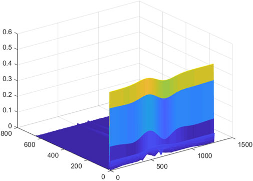
FIGURE 2. S-transformation 3D mesh graph of transient pulse signal.

FIGURE 3

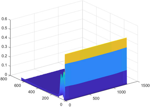
FIGURE 3. S-transformed 3D mesh graph of harmonic signal.

FIGURE 4

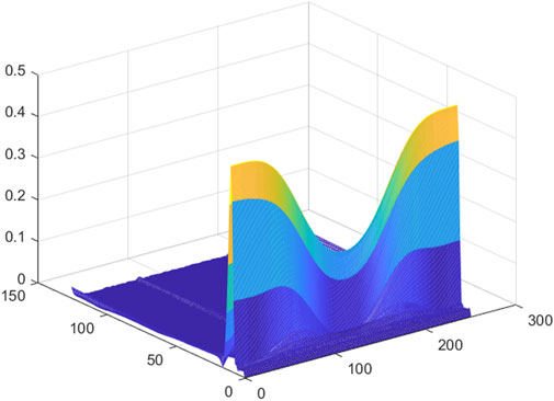
FIGURE 4. S-transformation 3D mesh graph of the sag signal.

FIGURE 5

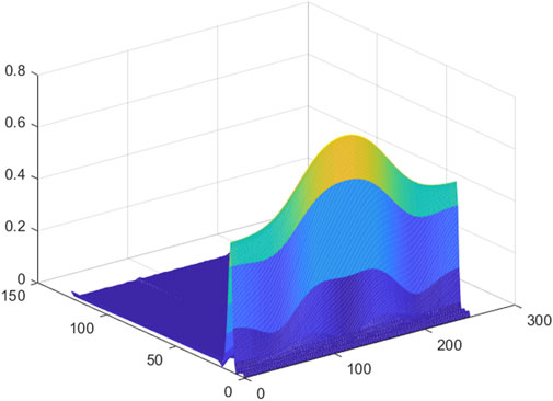
FIGURE 5. S-transformed 3D mesh graph of the swell signal.

FIGURE 6

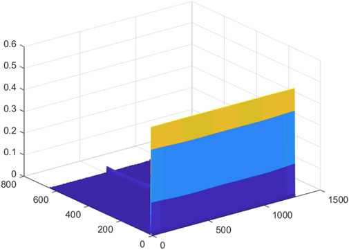
FIGURE 6. S-transformation 3D mesh graph of transient oscillation signal.

FIGURE 7

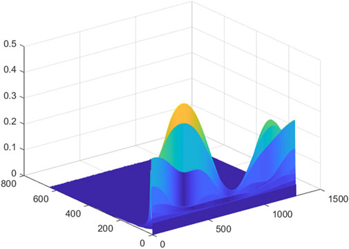
FIGURE 7. S-transformed 3D mesh graph of the interrupt signal.

FIGURE 8

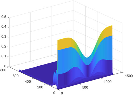
FIGURE 8. S-transformation 3D mesh graph of sag and harmonic signal.

Convolutional Neural Network

Convolutional Neural Network (CNN), as a deep learning method, has been widely used in the field of pattern recognition and image classification. The weight sharing mechanism of CNN is very similar to the model of biological neural network. This mechanism makes the network model simpler and greatly reduces the number of weights (Chen et al., 2018). CNN is mainly composed of input layer, convolutional layer, pooling layer (down-sampling layer), and fully connected layer.

CNN Network Structure and Principle

The common CNN network is the LeNet-5 network, and its structure is shown in Figure 9. The first few stages need to extract features through multi-layer convolution.

FIGURE 9

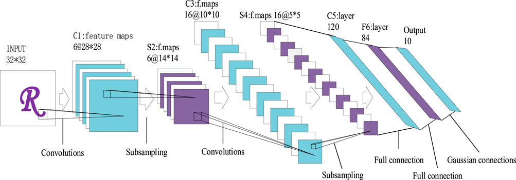
FIGURE 9. LeNet-5 structure chart.

The main components of CNN:

Convolutional layer: The purpose of the convolution operation is to extract different features of the input. The first convolutional layer may only extract some low-level features such as edges, lines, and corners. More layers of the network can iterate from the low-level features Extract more complex features.

Pooling layer: It is a form of downsampling. There are many different forms of non-linear pooling functions, of which Max-pooling and average sampling are the most common; the Pooling layer is equivalent to converting a higher resolution picture into a lower resolution picture; the pooling layer can Further reduce the number of nodes in the final fully connected layer, so as to achieve the purpose of reducing the parameters in the entire neural network.

Fully connected layer: The connection method is the same as that of a normal neural network, usually in the last few layers.

Generally speaking, CNN is a hierarchical model whose input is raw data, such as RGB images, raw audio data, etc. CNN extracts high-level semantic information from the original data through convolution, pooling, and nonlinear activation function mapping, and abstracts the original data layer by layer.

Convert the input raw data into the data form of a two-dimensional matrix, input it to the convolutional layer through the input layer, and use the convolutional layer to convolve the two-dimensional matrix. The calculation formula is as follows

$y_{\mathit{i}}^{\mathit{m}}=g\left({\displaystyle \sum }_{\mathit{j}=1}^{\mathit{k}}\mathit{conv2D}\left({\mathit{y}}_{\mathit{i}}^{\mathit{m}-1},{\mathit{\omega }}_{\mathit{ij}}^{\mathit{m}-1}\right)+{\mathit{b}}_{\mathit{i}}^{\mathit{m}}\right)(6)$

where $\mathit{g}\left(\right)$ is the activation function, $b_{\mathit{i}}$ is the bias value, ${\mathit{\omega }}_{\mathit{ij}}$ is the weight between neurons, and $y_{\mathit{i}}$ is the ith input of the neuron.

Due to the slow convergence speed of the saturated nonlinear function, and even the problem of the disappearance of the gradient in the back propagation stage, the excitation function in this paper adopts the ReLu nonlinear function, and its expression is as follows

$g\left(\mathit{x}\right)=\max \left(0,\mathit{x}\right)(7)$

After the original two-dimensional matrix is convolved by the convolution layer, the two-dimensional matrix obtained by the convolution operation is calculated by the ReLu activation function, and the calculated result is input to the pooling layer, and the downsampling operation is performed. As shown in the formula

$y_{\mathit{i}}^{\mathit{m}}=down\left(y_{\mathit{i}}^{\mathit{m}-1}\right)+b_{\mathit{i}}^{\mathit{m}}(8)$

where down() represents the downsampling function.

By merging and pooling, the dimensionality of the input feature matrix is reduced, and the calculation amount of the network model is reduced. The fully connected layer is used to transfer the weights and biases between neurons in each layer, and finally is classified by the SoftMax classification layer.

Network Training Process

The CNN training process consists of two stages: the forward propagation stage (Forward) and the backward propagation stage (Backward).

Forward propagation stage: The input signal is continuously processed by convolution, pooling and activation function in the forward propagation stage, and the output $\mathit{O}$ of the network is calculated layer by layer. Network calculation can be expressed as

$O=G_{\mathit{n}}\left(\cdots \left(G_2\left(G_1\left(X{W}_1\right)\right)W_2\right)\cdots W_{\mathit{n}}\right)(9)$

where $G_{\mathit{i}}$ represents the nonlinear transformation; and $W_{\mathit{i}}\left(i=\mathrm{1,2},\cdots ,n\right)$ represents the weight of each weight layer. After getting the network output O, use the ideal output Y to evaluate the CNN network, and the ideal network satisfies Y=O.

Back propagation stage: According to the network output obtained in the forward propagation stage, the error is calculated, and the expression is as follows

$E=\frac{1}{2}\Vert O-Y{\Vert }_2^2(10)$

The gradient descent method is used to update and optimize the weights and bias coefficients between neurons in each layer of the network to minimize errors. The update method of weight and bias in the network model is shown in the following formula

$W_{\mathit{ij}}^{\mathit{l}-1}\left(t+1\right)=W_{\mathit{ij}}^{\mathit{l}-1}\left(t\right)-\mathit{\eta }\frac{\partial \mathit{E}}{W_{\mathit{ij}}^{\mathit{l}-1}}(11)$

$b_{\mathit{j}}^{\mathit{l}}\left(t+1\right)=b_{\mathit{j}}^{\mathit{l}}\left(t\right)-\mathit{\eta }\frac{\partial \mathit{E}}{\partial {\mathit{b}}_{\mathit{j}}^{\mathit{l}}}(12)$

where $\mathit{\eta }$ represents the learning efficiency, E represents the error function.

CNN Parameter Settings

For different classification tasks, the determination of the CNN structure requires both theoretical analysis and experimental observation to select appropriate parameters. Each network contains a different number of convolutional layers and corresponding pooling layers, and the parameter settings of each convolutional layer and pooling layer are also different.

The convolution kernel parameters that need to be set are: stride (sliding step size), padding (convolution method) and the size of the convolution kernel. Stride should not be set too large, because too large will result in the loss of the feature amount of the input data, so stride is generally set to 1 or 2. There are two modes of padding setting: same and valid, same means that after the convolution operation, the dimensionality of the input data remains unchanged (0-padding is performed on the periphery of the input data according to stride’s value); valid means that the dimensionality of the input data will be reduced correspondingly after the convolution operation, and the size of the convolution kernel is determined according to the dimensions of the input data. The calculation method of the output data size is as follows

$U=\left[\frac{\left(I-C+2\ast P\right)}{\mathit{S}}\right]+1(13)$

where U is the size of the output data, I is the size of the input data, C is the size of the convolution kernel, P is the number of zero padding, and S is the size of the stride.

The sole purpose of the pooling layer is to reduce the dimensionality of the input data, and its parameter settings are: the selection of the pooling method, the size of the pooling layer and the sliding step length. Take an example to introduce the size and sliding step length of the pooling layer: input a 4×4 data, set the size of the pooling layer to 2×2, and set the step length to 2, and get an output 2×2 data after pooling. Figure 10 shows several common pooling methods.

FIGURE 10

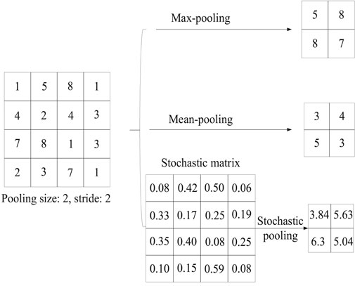
FIGURE 10. Common pooling methods.

Max-pooling only retains the maximum value in the area. Mean-pooling preserves the average value of the feature points in the area. Stochastic pooling only needs to randomly select the elements in the feature map according to their probability value, and the probability of element selection is positively related to its value. Among them, Max-pooling retains the maximum value, ignoring other values, which can reduce the impact of noise, improve the robustness of the model, reduce the number of model parameters, help reduce model overfitting problems, and be more suitable for power quality classification problems.

Example Construction

Mathematical Model of Power Quality Disturbance

The validity of real-time power quality disturbance data is affected by some other factors. For example, obtaining real-time power quality disturbance data requires a long monitoring time, and the location of the power quality disturbance event is uncertain, which greatly affects work efficiency. Therefore, using MATLAB to simulate the mathematical model of the power quality disturbance signal, the disturbance signal obtained by the simulation can accurately describe the real-time data in accordance with international standards (Chowdhury et al., 2016). Voltage sags, swells, spikes, interruptions, flickers, transient oscillations, harmonics, sags and harmonics, swells and harmonics are several common power quality disturbance signals. Attached schedule 1 is the model of 10 kinds of disturbance signals and standard signals, which are expressed as $S0,S1,\cdots S9$. among them $f=50Hz$; $\mathit{\omega }=2\mathit{\pi f}$; $T=\frac{1}{\mathit{f}}$.

Construction of Simulation Experiment Platform

This paper uses a two-dimensional CNN structure based on deep learning, uses TensorFlow deep learning framework, and Python 3.5 programming language to build a network model. The TensorFlow deep learning framework was built using a laptop equipped with a 64-bit Ubuntu Linux 16.04LTS system and NVIDIA GTX1080 graphics card. TensorFlow is an open-source software library that uses data flow graphs for numerical calculations. Its workflow is relatively easy, its API is stable, its compatibility is good, and it can be perfectly combined with NumPy. TensorFlow’s compilation time is very short, it can be iterated faster, and its flexibility and efficiency are relatively high. Using TensorFlow to build a two-dimensional convolutional neural network model, the program compilation is simple, the simulation speed is relatively fast, the flexibility is high, and it can be well adapted to the numerical optimization task.

The CNN Model Used in This Article

The CNN model used in this paper is improved based on the traditional LeNet-5 architecture model, including two convolutional layers and two pooling layers. The parameter settings of two convolution kernels are different, the specific parameter settings of the first convolution kernel: stride is set to 1, padding is set to same, the size of the convolution kernel is 3×3. The parameter settings of the second convolution kernel: stride is set to 1, padding is set to same, and the size of the convolution kernel is 5×5. The parameter settings of the two pooling layers are the same. The specific parameter settings are: Max-pooling is selected as the pooling method, the size of the pooling layer is 5×5, and the step size is set to 5. The dimension of the data input in this paper is 125×125, after the convolution and pooling operation, the dimension of the output data obtained is 5×5, and the output data obtained is input into the fully connected layer for normalization processing to avoid the impact of classification with large data values. Figure 11 shows the convolutional neural node pair network model used.

FIGURE 11

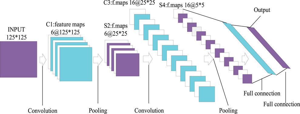
FIGURE 11. CNN model.

The cross-entropy loss function is used as the loss function of the CNN, and the SoftMax classification layer is used for classification. Figure 12 shows the system structure model of this article.

FIGURE 12

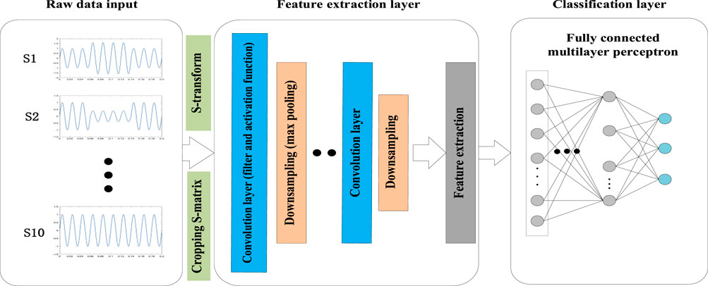
FIGURE 12. System structure model presented in this paper.

In the field of machine learning, if the model has too many parameters and the number of training samples is too little, it will lead to overfitting of the trained model. Overfitting often occurs in the training process of neural networks, the specific performance is: the model has a small loss function and high prediction accuracy on the training data, while on the test data, the loss function is relatively large and the prediction accuracy is low. In order to prevent the occurrence of overfitting, the CNN model used in this paper adds the Dropout function. In the process of forward propagation, the Dropout function allows a certain neuron to stop working with a certain probability, which can make the generalization ability of the neural network model stronger, so that it will not rely too much on some local features.

The role of the Dropout function:

1) Averaging effect: The Dropout removes neurons in different hidden layers is similar to training different networks, and the Dropout is equivalent to averaging multiple different neural networks.

2) Reduce the complex co-adaptation relationship between neurons: The update of weights no longer depends on the joint action of hidden nodes with fixed relationships, forcing the network to learn more robust features.

3) Dropout is similar to the role of gender in biological evolution: In order to survive, species tend to adapt to the new environment and can breed new species that adapt to the environment. This behavior is similar to training an applicable network model, which effectively prevents overfitting.

Disturbance Signal Classification Process

The flow diagram of the classification of power quality disturbance signals is shown in Figure 13.

FIGURE 13

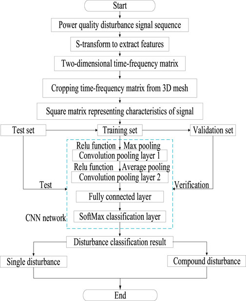
FIGURE 13. Process diagram of classification of power quality disturbance signals.

The specific steps are as follows:

1) Preprocess the power quality disturbance signal generated by MATLAB, use S-transform to extract the time-frequency matrix representing the disturbance signal, and draw a 3D network diagram of the disturbance signal.

2) According to the time-frequency matrix extracted from the 3D network graph of the disturbance signal, a new matrix of dimension 125×125 is obtained, and the training set is formed to train the CNN.

3) The cross-entropy loss function is adopted, and the Dropout function is added in the forward propagation stage to prevent the occurrence of overfitting. Use stochastic gradient descent method to update the parameter model, and optimize the model through error back propagation.

4) After the input data is convolved and pooled, the characteristics of the disturbance signal are extracted, and the SoftMax classification layer is used for classification. Then the verification and test sets are used for verification and testing to obtain the final classification results.

Simulation and Analysis

CNN Training

This article uses MATLAB to generate the power quality signals shown in Supplementary Table S1. Normal signals and every type of disturbance signal each generates 500 random samples, a total of 5,000 samples, each signal is added with a signal-to-noise ratio (SNR) of 20, 30 and 40dB Gaussian white noise. The feature matrix of all power quality signals is extracted from S-transform, and the feature matrix is trimmed using a 3D mesh graph. The trimmed feature matrix is integrated into a row of feature values by row, and a digital label is added to each row of data (0–9, respectively represent the labels of 10 disturbance signals). Shuffle all the data in rows and extract the first 3,000 rows of data from the disrupted data set to form the training set, the middle 1,000 rows of data form the verification set, and the last 1,000 rows of data form the test set. Use CNN to read the csv file containing the disturbance signal data.

In order to evaluate the training status and training effect of the network, the cross-entropy loss function and the classification accuracy rate are drawn with the number of iterations (each epoch represents training 50 times), namely the loss function curve and the classification accuracy curve. As shown in Figure 14, the loss function curve has a relatively large decline when the network is first trained. As the number of iterations increases, the loss function curve begins to fluctuate, but gradually stabilizes. As shown in Figure 15, the classification accuracy curve gradually increases as the number of iterations increases, and finally rises to a higher classification accuracy close to 1. As the number of iterations increases, the two curves gradually tend to converge, which proves that the entire network is continuously optimized and improved, and the stability of the network is gradually increasing. By comparing the classification effects of disturbance signals with different signal-to-noise ratios, it can be seen that the network still maintains a high classification accuracy rate for signals with different noises, indicating that the method has certain noise immunity and strong robustness.

FIGURE 14

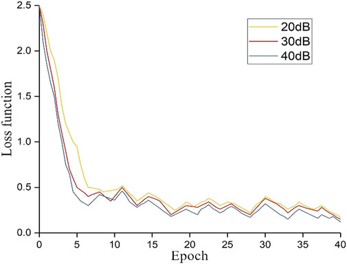
FIGURE 14. Training loss function curve.

FIGURE 15

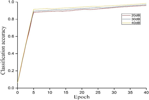
FIGURE 15. Classification accuracy curve.

Classification Effect

In order to further verify the effectiveness of this method, tests are performed under different noise intensities. The classification accuracy is shown in Table 1. It can be seen from Table 1 that CNN has higher accuracy under different noise intensities, indicating that the proposed method has strong noise immunity performance in the classification of power quality disturbance signals. In order to further determine the misclassification of disturbance signals, take the case of a signal-to-noise ratio of 40dB as an example, and list the classification results of each disturbance signal in the table below. It can be found that the classification accuracy of each signal is relatively high, and there is no excessive misclassification. The specific classification results of various disturbance signals are shown in Table 2.

TABLE 1

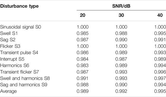
TABLE 1. Classification accuracy of CNN with different SNR.

TABLE 2

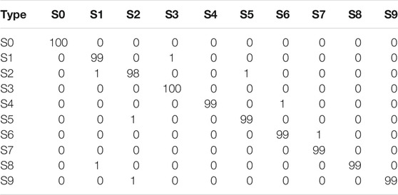
TABLE 2. Classification result details when the SNR is 40dB.

Comparative Analysis With Existing Classification Models

The proposed classification model and existing classification models are compared and analyzed to judge the classification effect of the classification model proposed in this paper. Models used for comparison include Probabilistic Neural Networks (PNN) (Zhengming et al., 2018), Principal Component Analysis-based Support Vector Machines (PCA-SVM) (Jiang et al., 2019a), and traditional Convolutional Neural Networks (CNN) (Song et al., 2018). The parameter setting of each model is set according to the existing reference documents, and will not be repeated here.

As shown in Table 3, it is the comparison result of the classification accuracy of different noise disturbance signals for each model. Comparing and analyzing the accuracy of different classification algorithms under different noise conditions, it is clear that the algorithm proposed in this article maintains a high classification accuracy rate under 20–40dB noise conditions. The results show that the classification accuracy of PNN and PCA-SVM is slightly lower than the model proposed in this paper. Since S-transform-CNN has an additional step of feature extraction using S transform, the model proposed in this paper has a higher classification accuracy and better noise immunity than traditional CNN model.

TABLE 3

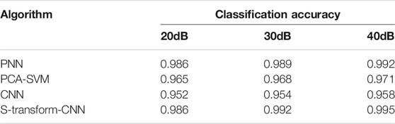
TABLE 3. Classification accuracy of different algorithms.

In addition to classification accuracy, this paper also compares classification time, the comparison results are shown in Table 4. It can be seen that the training time of PNN is relatively longer, because its structure is relatively complex and the number of neurons is relatively large, so the computational complexity is higher than the proposed method in this paper. The SVM in PCA-SVM belongs to binary classification, and the training and testing time is long. Since the proposed model has an extra feature extraction process compared with the traditional CNN, the training time is slightly longer.

TABLE 4

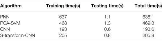
TABLE 4. Time consumption comparisons of different algorithms.

From the comprehensive analysis results of the above two tables, it can be seen that when considering the two factors of accuracy and time consumption, the classification accuracy of the S-transform-CNN method proposed in this paper is slightly lower than that of PNN, but the time consumed is much less than that of PNN. The reason is that the number of neurons in the PNN is relatively large, which greatly increases the computational complexity and the time consumed by the network. Among the existing disturbance signal classification methods, most of the classification methods focus on off-line detection and disturbance classification of power quality disturbance signals. As power quality problems become more and more complex and users have higher and higher requirements for power quality, it is necessary to conduct online analysis of power quality problems, and a shorter classification time is even more important. Considering comprehensively, the method proposed in this paper has higher classification accuracy and lower Time-consuming, which indicates that it can reduce the time of network training and testing and improve work efficiency while ensuring the classification accuracy.

Conclusion

This paper proposes a new method of power quality disturbance classification based on S-transform and CNN. Use S-transform to extract characteristics of disturbance signals, extract the time-frequency matrix representing the characteristics of the disturbance signal, then use the 3D mesh graph of the disturbance signal to trim the extracted matrix, and input the processed matrix into the CNN for classification. Under different noise levels, this method obtains relatively good classification accuracy for power quality disturbance signals, and has good noise immunity. The difference between this method and other methods based on CNN is the input form of the CNN. Traditional methods input the gray image of the disturbance signal. This paper directly inputs the characteristic matrix of the disturbance signal into the CNN. Compared with the traditional method, the method in this paper is more concise and reduces the loss of characteristics. Under the premise of ensuring classification accuracy and noise immunity. Further research will try to improve the performance of this method by introducing new feature extraction rules, and consider introducing more complex disturbance signals for classification to meet actual power quality analysis needs.

Data Availability Statement

The original contributions presented in the study are included in the article/Supplementary Material, further inquiries can be directed to the corresponding author.

Author Contributions

JL conceived the idea for the manuscript and wrote the manuscript with input from HL, DW, and TB. All authors have read and agreed to the published version of the manuscript.

Conflict of Interest

The authors declare that the research was conducted in the absence of any commercial or financial relationships that could be construed as a potential conflict of interest.

Supplementary Material

The Supplementary Material for this article can be found online at: https://www.frontiersin.org/articles/10.3389/fenrg.2021.708131/full#supplementary-material

References

Chowdhury, A. R., Lin, T.-Y., Maji, S., and Learned-Miller, E., (2016). "One-to-many Face Recognition with Bilinear CNNs," in 2016 IEEE Winter Conference on Applications of Computer Vision (WACV), pp. 1–9. doi:10.1109/WACV.2016.7477593

CrossRef Full Text | Google Scholar

Chang, L., Deng, X. M., and Zhou, M. Q., (2016). Convolutional Neural Networks in Image Understanding. Acta Automatica Sinica 42 (9), 1300–1312. doi:10.16383/j.aas.2016.c150800

CrossRef Full Text | Google Scholar

Chen, W., He, J., and Pei, X. (2018). Classification for Power Quality Disturbance Based on Phase-Space Reconstruction and Convolution Neural Network. Dianli Xitong Baohu Yu Kongzhi/Power Syst. Prot. Control. 46 (14), 87–93. doi:10.7667/PSPC171080

CrossRef Full Text | Google Scholar

Deng, H., Gao, Y., Chen, X., Zhang, Y., Wu, Q., and Zhao, H. (2020). “Harmonic Analysis of Power Grid Based on FFT Algorithm,” in 2020 IEEE International Conference on Smart Cloud (SmartCloud), 161–164. doi:10.1109/SmartCloud49737.2020.00038

CrossRef Full Text | Google Scholar

Dhoriyani, S. L., and Kundu, P. (2020). “Comparative Group THD Analysis of Power Quality Disturbances Using FFT and STFT,” in 2020 IEEE First International Conference on Smart Technologies for Power (Energy and Control (STPEC)), 1–6. doi:10.1109/STPEC49749.2020.9297759

CrossRef Full Text | Google Scholar

Haddad, R. J., Guha, B., Kalaani, Y., and El-Shahat, A. (2018). Smart Distributed Generation Systems Using Artificial Neural Network-Based Event Classification. IEEE Power Energ. Technol. Syst. J. 5 (2), 18–26. doi:10.1109/JPETS.2018.2805894

CrossRef Full Text | Google Scholar

Hezuo, Q. U., Xiaoming, L. I., and Chen, C., (2018). Classification of Power Quality Disturbances Using Convolutional Neural Network. Engineering Journal of Wuhan University.

Huang, B., Li, Y., Zhan, F., Sun, Q., and Zhang, H. (2021). A Distributed Robust Economic Dispatch Strategy for Integrated Energy System Considering Cyber-Attacks. IEEE Trans. Ind. Inf., 1in press. doi:10.1109/TII.2021.3077509

CrossRef Full Text | Google Scholar

Huang, B., Liu, L., Li, Y., and Zhang, H. (2019). Distributed Optimal Energy Management for Microgrids in the Presence of Time-Varying Communication Delays. IEEE Access 7, 83702–83712. doi:10.1109/ACCESS.2019.2924269

CrossRef Full Text | Google Scholar

Huang, N., Zhang, W., and Cai, G., (2015). Power Quality Disturbances Classification with Improved Multiresolution Fast S-Transform. Power Syst. Tech. 39 (05), 1412–1418. doi:10.13335/j.1000-3673.pst.2015.05.036

CrossRef Full Text | Google Scholar

Jahangir, H., Tayarani, H., Baghali, S., Ahmadian, A., Elkamel, A., Golkar, M. A., et al. (2020). A Novel Electricity Price Forecasting Approach Based on Dimension Reduction Strategy and Rough Artificial Neural Networks. IEEE Trans. Ind. Inf. 16 (4), 2369–2381. doi:10.1109/TII.2019.2933009

CrossRef Full Text | Google Scholar

Jiang, G., He, H., Yan, J., and Xie, P. (2019). Multiscale Convolutional Neural Networks for Fault Diagnosis of Wind Turbine Gearbox. IEEE Trans. Ind. Electron. 66 (4), 3196–3207. doi:10.1109/TIE.2018.2844805

CrossRef Full Text | Google Scholar

Jiang, J., Wen, Z., Zhao, M., Bie, Y., Li, C., Tan, M., et al. (2019a). Series Arc Detection and Complex Load Recognition Based on Principal Component Analysis and Support Vector Machine. IEEE Access 7, 47221–47229. doi:10.1109/ACCESS.2019.2905358

CrossRef Full Text | Google Scholar

Kumar, R., Singh, B., Shahani, D. T., Chandra, A., and Al-Haddad, K. (2015). Recognition of Power-Quality Disturbances Using S-Transform-Based ANN Classifier and Rule-Based Decision Tree. IEEE Trans. Ind. Applicat. 51 (2), 1249–1258. doi:10.1109/TIA.2014.2356639

CrossRef Full Text | Google Scholar

Long, J. (2018). Feature Extraction and Classification of UHF PD Signals Based on Improved S-Transform. Gaodianya Jishu/High Voltage Eng. 44 (11), 3649–3656. doi:10.13336/j.1003-6520.hve.20181031026

CrossRef Full Text | Google Scholar

Luo, Y., Li, K., Li, Y., Cai, D., Zhao, C., and Meng, Q. (2018). Three-Layer Bayesian Network for Classification of Complex Power Quality Disturbances. IEEE Trans. Ind. Inf. 14 (9), 3997–4006. doi:10.1109/TII.2017.2785321

CrossRef Full Text | Google Scholar

Niu, S., Wang, K., and Liang, Z. (2019). Synchronous Phasor Estimation Method for Power System Based on Modified Strong Tracking Unscented Kalman Filter. Power Syst. Tech. 43 (09), 3218–3225. doi:10.13335/j.1000-3673.pst.2018.2814

Google Scholar

Qiu, W., Tang, Q., Liu, J., and Yao, W. (2020). An Automatic Identification Framework for Complex Power Quality Disturbances Based on Multifusion Convolutional Neural Network. IEEE Trans. Ind. Inf. 16 (5), 3233–3241. doi:10.1109/TII.2019.2920689

CrossRef Full Text | Google Scholar

Sai, T. K., and Reddy, K. A. (2015). New Rules Generation from Measurement Data Using an Expert System in a Power Station. IEEE Trans. Power Deliv. 30 (1), 167–173. doi:10.1109/TPWRD.2014.2355595

CrossRef Full Text | Google Scholar

Song, H., Dai, J., and Zhang, W., (2018). Partial Discharge Pattern Recognition Based on Deep Convolutional Neural Network under Complex Data Sources. Gaodianya Jishu/High Voltage Eng. 44 (11), 3625–3633. doi:10.13336/j.1003-6520.hve.20181031023

CrossRef Full Text | Google Scholar

Stockwell, R. G., Mansinha, L., and Lowe, R. P. (1996). Localization of the Complex Spectrum: the S Transform. IEEE Trans. Signal. Process. 44 (4), 998–1001. doi:10.1109/78.492555

CrossRef Full Text | Google Scholar

Sun, Y., Tang, X., and Sun, X., (2018). Research on Multi-type Energy Storage Coordination Control Strategy Based on MPC-HHT. Proc. CSEE 38 (09), 2580–2588. doi:10.13334/j.0258-8013.pcsee.171042

Google Scholar

Tang, Q., Qiu, W., and Zhou, Y. (2020). Classification of Complex Power Quality Disturbances Using Optimized S-Transform and Kernel SVM. IEEE Trans. Ind. Electron. 67 (99), 9715–9723. doi:10.1109/TIE.2019.2952823, PP(

CrossRef Full Text | Google Scholar

Thirumala, K., Prasad, M. S., Jain, T., and Umarikar, A. C. (2018). Tunable-Q Wavelet Transform and Dual Multiclass SVM for Online Automatic Detection of Power Quality Disturbances. IEEE Trans. Smart Grid 9 (4), 3018–3028. doi:10.1109/TSG.2016.2624313

CrossRef Full Text | Google Scholar

Wang, F., Quan, X., and Ren, L., (2021). Review of Power Quality Disturbance Detection and Identification Methods. Proc. CSEE 1-17. in press. http://kns.cnki.net/kcms/detail/11.2107.TM.20201119.0900.002.html.

Google Scholar

Wang, R., Sun, Q., Gui, Y., and Ma, D. (2019). Exponential-function-based Droop Control for Islanded Microgrids. J. Mod. Power Syst. Clean. Energ. 7 (4), 899–912. doi:10.1007/s40565-019-0544-3

CrossRef Full Text | Google Scholar

Wang, R., Sun, Q., Tu, P., Xiao, J., Gui, Y., and Wang, P. (2021a). Reduced-Order Aggregate Model for Large-Scale Converters with Inhomogeneous Initial Conditions in DC Microgrids. IEEE Trans. Energ. Convers., 1in press. doi:10.1109/TEC.2021.3050434

CrossRef Full Text | Google Scholar

Wang, Y., Li, Q., and Zhou, F. (2017). A Novel Algorithm for Transient Power Quality Disturbances Detection. Proc. CSEE 37 (24), 7121–7132. doi:10.13334/j.0258-8013.pcsee.162592

CrossRef Full Text | Google Scholar

Yong, D. D., Bhowmik, S., and Magnago, F. (2015). An Effective Power Quality Classifier Using Wavelet Transform and Support Vector Machines. Expert Syst. Appl. 42 (15-16), 6075–6081. doi:10.1016/j.eswa.2015.04.002

CrossRef Full Text | Google Scholar

Zhengming, L. I., Qian, L., and Jiabin, L. I. (2018). Type Recognition of Partial Discharge in Power Transformer Based on Statistical Characteristics and PNN. Power Syst. Prot. Control. 46 (13), 55–60. doi:10.7667/PSPC170962

CrossRef Full Text | Google Scholar

Zhou, L., Guan, C., and Lu, W. (2011). Application of Multi-Label Classification Method to Catagorization of Multiple Power Quality Disturbances. Zhongguo Dianji Gongcheng Xuebao/Proceedings Chin. Soc. Electr. Eng. 31 (4), 45–50. doi:10.1631/jzus.C1000008

CrossRef Full Text | Google Scholar

Zhu, Ruijin., Guo, Weilin., and Gong, Xuejiao. (2019). Power Quality Disturbance Classification Based on Self Encoder and Convolutional Neural Network. J. Power Syst. automation 31, 70–75. doi:10.19635/j.cnki.csu-epsa.000199

CrossRef Full Text | Google Scholar