 Ke Yang
 Shuiqing Zhou1,2*
95% of researchers rate our articles as excellent or good
Learn more about the work of our research integrity team to safeguard the quality of each article we publish.
Find out more
ORIGINAL RESEARCH article
Front. Energy Res. , 23 June 2021
Sec. Process and Energy Systems Engineering
Volume 9 - 2021 | https://doi.org/10.3389/fenrg.2021.700365
This article is part of the Research Topic Emerging Sustainable and Energy-Efficient Technologies in Heat Pumps for Residential Heating View all 9 articles
As one of the key components of the heat pump system, compared to that of a conventional axial fan, the blade tip area of a forward-swept axial fan is much larger than its blade root, which is the main noise source of the fan and also has an important influence on the fan efficiency. Enhancement of the aerodynamic performance and efficiency of a forward-swept axial fan was addressed by utilizing the Bezier function to parameterize the forward-swept curve on blade tops. In order to quickly select an agent model suitable for the project, an ES model was established by integration of the radial basis function model and the Kriging model. When NSGA-II was combined, multi-objective optimization was carried out with the flow rate and total pressure efficiency as optimization goals. Analysis of optimization results revealed that the optimized axial flow fan’s flow rate and total pressure efficiency were improved to some degree. At the design working point, the fan’s flow rate increased by 1.78 m³/min, while the total pressure efficiency increased by 3.0%. These results lay solid foundation for energy saving of the heat pump system.
Nowadays, an air-conditioning refrigeration system and a heat pump system are widely used as temperature-regulating equipment by people all over the world. Heat pumps are heavily used in a cold climate (Xu et al., 2020). Due to the extensive use of related equipment, they have led to huge energy consumption and considerable greenhouse gas emissions while improving people’s quality of life (Xu et al., 2021). As climate warming and energy problems become increasingly prominent, relevant institutions attach more and more importance to energy and have issued corresponding standards (CONTROLS, REFRIGERATION).
The axial flow fan is the main component of an air-conditioning system and a heat pump system. Improving its working efficiency can effectively reduce the energy consumption of the temperature regulation system (Usman et al., 2017). At the same time, its aerodynamic performance has a great impact on the overall performance of the air-conditioning system and heat pump system and determines the user’s comfort level (Lim et al., 2020). According to vortex-sound theory, turbulent vortexes are the main influence factor of fan noise, so the turbulence vortexes generated by unreasonable flow inside the fan will greatly affect the efficiency of the fan. Therefore, sound is a form of energy dissipation, and optimizing fan noise can indirectly improve the efficiency of the fan (Schram and Hirschberg, 2003). At the same time, excessive noise will affect user experience. Therefore, in order to make more efficient use of energy, designers put forward higher requirements for the aerodynamic performance of axial flow fans, and the goal of making high efficiency, low noise, and large flow rate is to be pursued (Jung and Joo, 2019). Because the blade is the main power element of the axial fan, it is of great significance to explore the feasibility of its parameter optimization for the improvement of energy efficiency of a heat pump.
Various scholars have conducted extensive research on improving axial flow fan performance. Xie et al. (2019) have explored the influence of various forward-swept angles on performance parameters of axial flow fans based on a parameterized model of various forward-swept angles in cooling fans, and the results show that the average air pressure at the inlet increases continuously and the air velocity increases with the increase in the forward sweep angle of the fan. Using the non-uniform rational B-spline (NURBS) parameterization method, Liu et al. (2019) have modified axial flow fan blade profiles, and under the off-design condition, the aerodynamic performance of the axial fan is greatly improved. Through experiments and numerical simulations, Hurault et al. (2010) have assessed the effects of forward-swept designs of axial flow fans on the flow field turbulent kinetic energy, and the sweep has a significant influence on the turbulent kinetic energy downstream of the fan. Ding et al. (2019), Lin et al. (2014), Angelini et al. (2017), Lin et al. (2014), Angelini et al. (2017), and Ding et al. (2019) have further implemented a parametric optimization design based on the Bezier curve for various forms of fluid machinery. Meanwhile, Ye (2017) has optimized an underwater glider wing type based on an agent model technology.
On the contrary, there are many scholars at home and abroad to optimize fluid machinery by combining the agent model and the optimization algorithm after parameterization of the optimization target. Della Vecchia et al. (2014) used Parsec for parameterized characterization of an airfoil, combined with genetic algorithms (GAs) for optimization design, and thus obtained a winged type with good aerodynamic performance. Zhou et al. (2021) used Hicks-Henne bump functions to conduct parameterized characterization of the blades of a multi-blade centrifugal fan and combined the Kriging approximate model and NSGA-II to conduct multi-objective optimization design of the blades. After optimization, the aerodynamic performance of the blades has been significantly improved. Yang and Xiao (2014) parameterized the impeller of the pump and combined the RSM model and MGA to carry out multi-objective optimization design of the impeller, and the hydraulic performance of the pump after optimization has been significantly improved.
The aforementioned studies have included hubs of low-speed axial fans that are relatively small and have few blades. The chord length, thickness, and attack angle of various blade heights vary extensively, such that the boundary layer on the wall surface is relatively thin, leading to separation flow along the blade leading edge (Zhou et al., 2014). With the increase in load, the power capacity of the blade tip can be improved, and then the fan efficiency can be improved (T, 2017). In severe cases, channel obstruction and rotation stall are some of the consequences (Zhou, 2015). Accordingly, a parametric optimization design method can enhance an axial flow fan’s blade performance, but there are currently few reports regarding fan optimization using the Bezier curve, which can be combined with a parametric optimization design and applied to the blade tip of a forward-swept axial fan. Compared to typical axial flow fans, a blade sweep design has a certain influence in mitigating flow loss. From the static pressure distribution on the blade surface, the forward-swept moving blade increases the load distribution of the upper blade height and enhances the power capacity of the blade. The forward-swept design can reduce the turbulent kinetic energy at the blade tip and reduce the clearance flow loss (Zhang et al., 2019). The blade tip areas of forward-swept axial flow fans are much larger than their blade roots and serve as the main working areas as well as noise sources (Yang and Chen, 2002). Utilizing cubic-Bezier applications to parameterize the forward-swept curve on the blade top and selecting the flow rate and total pressure efficiency as optimization goals, this study examined the relationship between the tip sweep curve and optimization goals. The radial basis function (RBF) and Kriging models were integrated to establish an ensemble of surrogates to improve the optimization efficiency and reduce the sample size, non-dominated sorting genetic algorithm II (NSGA-II) was selected for optimizing the blade tip forward sweep curve, and numerical simulations were employed to explore shifts in the flow field and acoustic attributes before and after optimization.
In this study, the optimization object was a heat pump axial flow fan (Figure 1). A semi-open axial flow impeller is primarily used in outdoor air-conditioning units. Its fundamental parameters are the impeller outer diameter at 401 mm, hub ratio 0.25/1, tip clearance 6 mm, blade number 3, h = 150.75 mm, L/h = 19.3%, impeller speed 839 rpm, flow rate 29.7 m³/min, and noise level 50.9 dB. Profile data at various blade height sections are provided in Table 1.
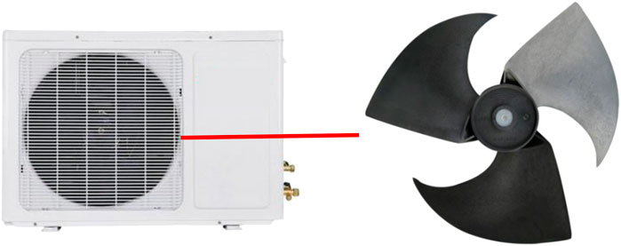
FIGURE 1. Axial flow fan model.
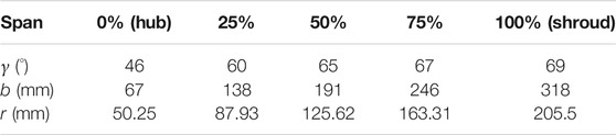
TABLE 1. Profile data.
The blade radial profile was modified to improve the pressure distribution at the tip by changing the forward sweep curve of the blade tip on the premise that the profile accumulation and geometry of the blade below 75% of blade height were exactly the same. The cubic-Bezier function with smooth curvature was used for parametrically designing forward sweep curves of >75% blade height (Figure 2). The Bezier curve had four nodes, and its equation is expressed as
where
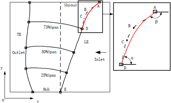
FIGURE 2. Parameterization of an axial fan blade profile.
The parametric design was facilitated by taking angles as design variables. The angles included the angle between C–D and the axis and between A–B and the axis, with endpoint A at
It was then obtained that
where I is the unit vector in the x-direction.
Thus, it was considered that the parameterization problem was controlled by the equation
Then, the known α and β angles and the Y coordinates of points B and C were substituted into the above formula to determine the X coordinates of points B and C. Finally, according to the determined vertex coordinates of the control polygon, the entire cubic-Bezier curve was obtained and the blade profile was determined. Automatic modeling was facilitated by compiling the above process into code and using MATLAB to output the desired curve, and 3D modeling software was imported to obtain the blade model after parameter changes.
The fan’s geometric model was established using three-dimensional (3D) modeling software. The model file was then imported into pre-processing software for simplification. The fluid domain of the whole fan was divided into three regions, the inlet, fan, and outlet. For accurate calculation of the axial flow fan’s import and export flows, its basin became an appropriate extension of its imports and exports. The import basin was along the inlet’s direction, thus extending the length of the axial flow fan to five times the wheel rim diameter. The basin was further extended along the fan’s export direction, thus likewise lengthening the axial flow fan to five times the rim diameter. This was intended to mitigate the outlet air flow of the axial flow fan, which could influence internal air flow (Wang, 2004).
The blade of an axial flow fan rotates at high speed and the internal flow field is complex, such that the quality of the computational grid is required to be higher. Here, calculation accuracy was ensured by adopting a full-flow channel hexahedron-structured grid in the axial flow fan and the fan area grid locally encrypted (Figure 3).
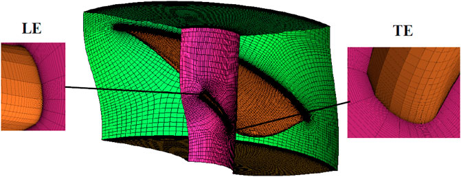
FIGURE 3. Calculation model.
This study applied computational fluid dynamics (CFD) numerical simulation software to solve the internal flow field of an axial flow fan. Dry air at 25°C was selected as the working fluid, the impeller fluid domain was set as the rotating region, and a multi-reference frame model was adopted, with other basins fixed. The blade was set as a moving wall; inlet and outlet boundary conditions were set as the pressure inlet and outlet, respectively; and the outlet was set as the flow-monitoring surface. The solution used the realizable k-ε model. The SIMPLE algorithm, which has strong universality, was selected as the velocity and pressure coupling mode. Momentum, dissipation rate, and turbulent kinetic energy equations in the second-order upwind format were used for the spatial discrete format. The RMS value of the governing equation was specified to be < 10–5 to guarantee an accurate convergence criterion.
The turbulence state at the fan inlet and outlet was defined by the turbulence intensity I and outlet diameter DH. The turbulence intensity I was estimated according to the empirical formula of turbulence intensity, expressed as
Here, the inlet and outlet turbulence intensities were estimated at 4% and all solid walls were assumed to be slippage free.
When dividing the grid, the first node should be placed in the viscous region at the bottom, where the y+ value was generally considered to be < 5. The empirical formula of y+ was
where Ywall is the height of the first layer of the boundary layer grid, in mm; Vref is the reference speed, in m/s; Lref is the reference length, in m; ν is the fluid kinematic viscosity, in m2/s; and y+ is a dimensionless parameter, indicating the boundary point between the viscous bottom and logarithmic layers. Therefore, the height of the first layer of the boundary layer grid should be <0.44 mm.
With around 2.5 million meshes, the total pressure varies within 1% (Figure 4). Thus, comprehensively considering calculation precision and time, the calculated grid number here was determined to be 2476811.
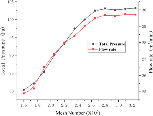
FIGURE 4. Grid independence verification.
This study calculated the parallel system of microcomputer cluster using a 384-core CPU, equipped with eight Sugon computing nodes, and the peak computing capacity reached 36.86 Tflops. Each computing node was equipped with two latest Intel 6248R CPUs, with a total memory of up to 3T, and InfiniBand was used for high-speed data exchange between computing nodes, such that cluster computing met the present computing needs.
The aerodynamic performance of the axial fan was tested using a standard air duct under international standard GB∕T 1236-2017 (GB∕T 1236-2017, 2017). A schematic diagram of the test bench for measurements is shown in Figure 5, with testing accuracy at ±1%.
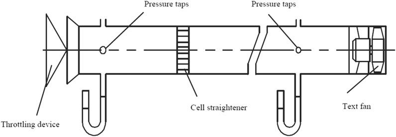
FIGURE 5. Aerodynamic performance test device diagram.
The obtained numerical and experimental performance curves agreed well with the large flow area (Figure 6). However, in the small flow rate region, the error was a little large, which was due to numerical simulation of turbulence and boundary layer separation being difficult. The design flow condition error was 4%, which was within the acceptable range (Ravelet et al., 2018).
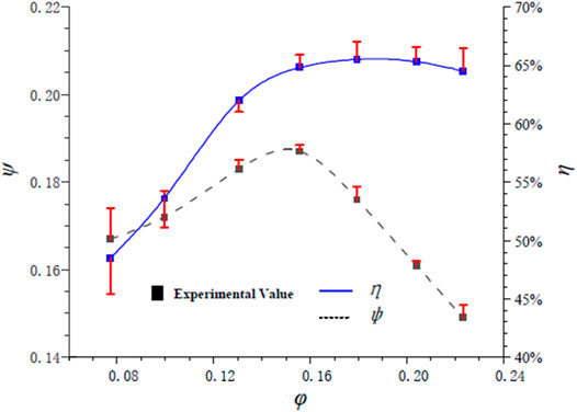
FIGURE 6. Comparison of test and numerical simulation performance curves.
The Opt LHD method was used in experiments (Zapotecas and Coello, 2013), and this method design made all test points evenly distributed in the design space as far as possible, with very good space filling and equilibrium.
For the 23 groups of sample points designed by the Opt LHD experiment, the curve of the blade profile centerline of each sample point was uniformly plotted and the samples obtained by the experiment design were observed to have good space filling. Each group of sample points and their related flow rates and total pressure efficiencies were recorded, and the sample points were modeled through numerical simulation.
The sample points are also shown in Figures 7, 8. Although 23 sets of variables were obtained and the corresponding response sample data through the Opt LHD method combined with a large number of numerical simulation calculations, this was still only the sampling result of sample points in the value interval of each variable. The corresponding response of any target point in the predictive variable interval was predicted by solving the performance response at any other unknown point, based on the obtained sampling data sample and the relevant mathematical prediction model. The 23 samples of forward-swept line are shown in Figure 9.
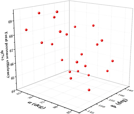
FIGURE 7. Opt LHD test design (
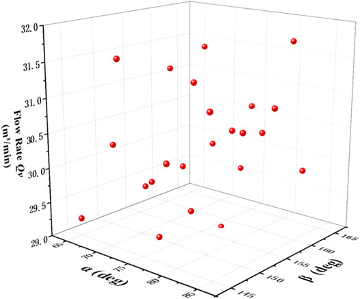
FIGURE 8. Opt LHD test design (
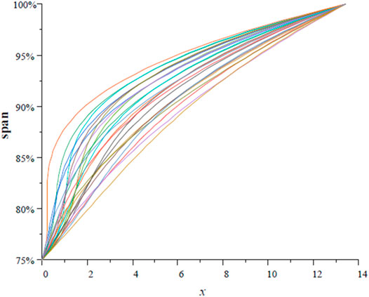
FIGURE 9. Samples of Opt LHD.
Due to the limitations of computation and complexity in engineering optimization, if each generated fan model adopts the CFD method to solve the response target, the workload is huge. Here, the optimization effort and cost were reduced using agent model technology, which is usually used to construct explicit function relationships between input parameters and output response. For the unpredictability of optimization problems, it is difficult for researchers to quickly select an appropriate agent model, which results in reductions in model accuracy and optimization efficiency (Jin et al., 2000; Du, 2018). Therefore, two classical agent models, RBF and Kriging models, were applied here to solve this problem by forming an ensemble of surrogates (ES) (Goel et al., 2007) and make the best use as possible of each agent model.
The ES is a linear weighted combination function of several agent models, and its mathematical expression was
where
To avoid the agent model in the sparse area of the sample prediction ability is poor, the weight factor size is needed to reflect the corresponding agent model accuracy. Therefore, here, PRESSRMS was used to calculate
where m is the chosen agent model, Ei is the agent model’s PRESSRMS of number I, and
After obtaining the weight factors of the single agent model, the mathematical expression for the ES was
The bivariate multimodal function was then used to verify the reliability of the combined agent model:
The uncertainty generated during the test was reduced and the test universality was increased by generating training sample points using the optimal Latin hypercube design (Opt LHD) method to generate training sample points. Using these points and the calculated true objective function values, single agent models of RBF and Kriging models, respectively, were constructed for the test function. After completing agent model construction, the PRESSRMS of different agents and their weight factors were calculated. The ES was obtained through a weighted summation of the corresponding agent models. For the fitting function using single RBF and Kriging models (Figures 10A, 11A), it was found that the RBF and Kriging models could well predict the shape of the real function graph (Figures 10B, 11B). These models had slightly larger errors in prediction values at the boundary, and the error value in the middle portion was relatively stable. Also, the fitting function of the ES model weighted by the RBF and Kriging models showed that the ES model also well predicted the shape of the real function graph (Figure 12A). The prediction error at the boundary was also slightly decreased, and in particular, the errors at the four base angles were significantly decreased and the error in the middle part was basically unchanged (Figure 12B). Therefore, the ES model was more reliable than the single agent model for the fitting of unknown functions.
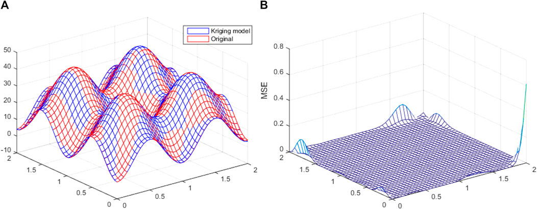
FIGURE 10. RBF model. (A) Comparison between the RBF model and the real function. (B) Mean square error (MSE).

FIGURE 11. Kriging model. (A) Comparison between the Kriging model and the real function. (B) Mean square error (MSE).
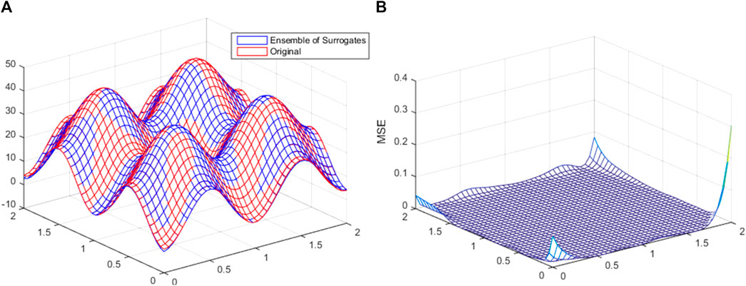
FIGURE 12. ES. (A) Comparison between the ES and the real function. (B) Mean square error (MSE).
The first 20 sets of data generated by the Opt LHD method were taken as the initial samples, and the initial sample points were added to the training sample set. The program was set to output the corresponding fan geometric model, and the target response function value of the initial sample points was calculated by the high-precision simulation analysis model.
The agent model was adopted to establish the objective function, but, first, clear constraints were required. Changing the forward-swept angle in a small range could significantly improve aerodynamic efficiency, but the effects are not as obvious if the angle continues to increase (Cai, 1997; Liu, 2008). Therefore, to ensure the forward-swept characteristics of the curve, the experience rule was referred to produce an angle range of α, β:
At the same time, the PRESSRMS predicted by the two agent models (RBF and Kriging models) was calculated using Eqs. 8, 9 to obtain the weight factors
Therefore, the entire optimization process is shown in Figure 13.
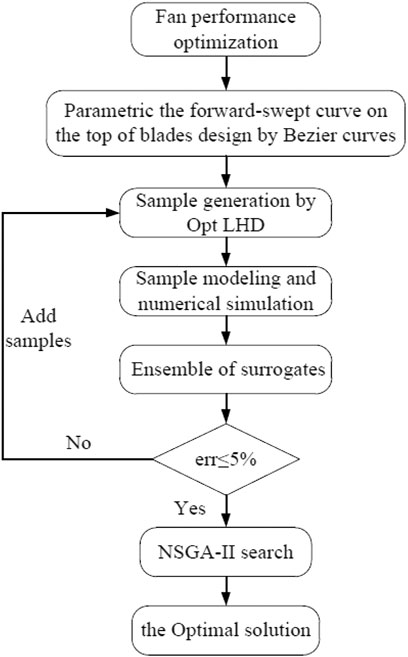
FIGURE 13. Optimization process.
The optimization objectives of the fan in this study include the total pressure efficiency and flow rate, forming a typical multi-objective optimization problem. In this case, it was impossible to optimize the total pressure efficiency and flow rate at the same time. Each goal was interrelated, and the optimal value of one goal might have diminished the optimal value of another goal. Thus, it was necessary to make each target close to the optimal value at the same time.
Due to the limitations of parameter selection, there will be some errors in the combined agent model. The accuracy of the model was verified by testing the relevant accuracy test formula before the prediction solution. Here, the correlation coefficient R2 was used to determine the accuracy of the approximate model. The equation for R2 calculation was
where i is the sample number; n is the total number of samples; y̅ is the average value of the test samples; and ŷ is the predicted value of the test sample. The closer the R2 to 1, the better the ES model fit.
The last three sets of 23 sample points designed by the above Opt LHD experiment were taken as test samples to verify the accuracy of the established ES model. Under the same setting parameters, the numerical simulation value of the sample points was solved to obtain the response of each sample point. Combined with the response of each point predicted by the ES model, the phase relation value of the model was solved (Table 2). The R2 values of the total pressure efficiency and flow rate of the model were both greater than 0.95, which demonstrated that the model possessed good accuracy.
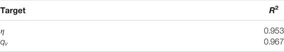
TABLE 2. R2 terms.
NSGA-II based on an elite retention strategy is a classic algorithm for solving this type of multi-objective problem, with comprehensive advantages in solving quality and convergence efficiency (Srinivas and Deb, 1994).
NSGA-II was used to make the individual fully extend to the whole Pareto computing domain and avoid falling into the local optimal solution. The population size was set to 100, iterations to 1,000, and crossover probability and mutation probability to 0.7 and 0.3, respectively.
Figure 14 shows the Pareto front. It can be seen that the gap between the solution sets is small. In the optimization process, the flow rate
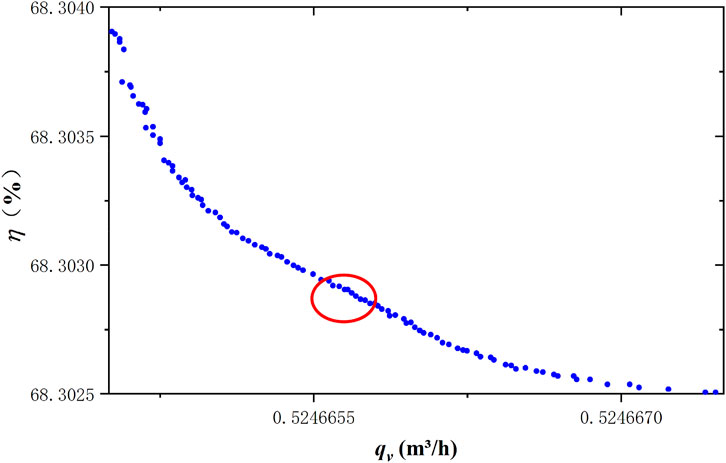
FIGURE 14. Pareto front.
The structural parameters corresponding to the optimal solution and the total pressure efficiency and flow rate at the design condition point showed that, at the design working point, the effective air volume of the fan increased by 1.78 m³/min and the total pressure efficiency increased by 3.0% (Table 3). And a comparison of the blade profile before and after the optimization is shown in Figure 15.
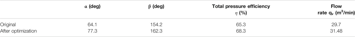
TABLE 3. Structural parameters corresponding to the optimal solution.
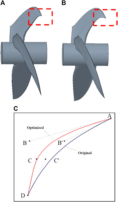
FIGURE 15. Comparison of blade profiles before and after optimization. (A) Original. (B) Optimized. (C) Comparison of two blade profiles.
Comparing the fan performance curves before and after optimization, the efficiency of the optimized fan is obviously higher than that of the original one, and a higher efficiency fan can save the energy of the heat pump system (Figure 16). The influence of internal flow field changes on fan performance and efficiency after blade optimization was further studied by analyzing the flow field inside the fan before and after optimization at the design working point in terms of its effects on overall fan performance.
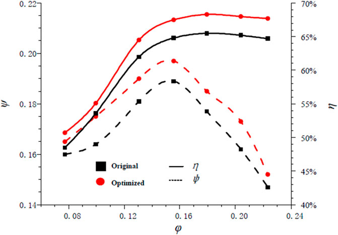
FIGURE 16. Original and optimized fan performance curves.
According to the average velocity contour distribution of a series of different leaf height positions, the optimized model gas flow was seen to be fully attached to the blade (Figure 17). The tip speed of the optimized model increased, indicating that the optimized profile increased the load in the tip area as well as the blade functional capacity. This was also an important reason for the improved total pressure efficiency of the optimized fan.
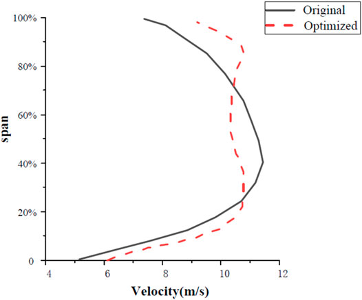
FIGURE 17. Original and optimized average velocity isoline distributions at different blade heights.
Details of the flow in the axial flow fan channel were revealed by examining the velocity distribution of the S2 flow surface before and after optimization, with the separated vortex flow occupying the gas flow section of the axial flow fan and the gas flow angle changing during the flow process (Figure 18). Part of the flow vector direction of the original model near the blade outlet was clearly seen to be shifted, which had an impact on the trailing edge with a higher blade spread height. After the blade tip sweep curve was optimized by the Bezier function, observation of the separation flow in the impeller passage showed that the center of the passage vortex shifted to the exit direction. As the separation flow area was smaller, the main flow direction was weakened by the influence of the passage vortex and the flow did not deviate significantly. Therefore, the flow distribution of the optimized axial flow fan is improved, and the unnecessary energy loss is avoided and the fan efficiency is improved.
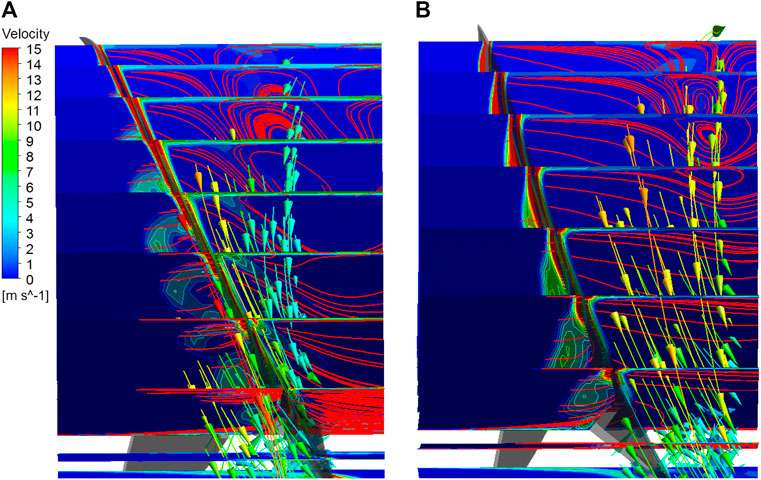
FIGURE 18. Velocity distribution of the S2 flow surface. (A) Original. (B) Optimized.
According to vortex-sound theory, turbulent vortexes are the main influence factor of fan noise. For isentropic flows at low Mach number, the vortex-acoustic equation is
where B is the total enthalpy of the fluid, w is the flow vortex vector, and v is the velocity vector. The basic factors leading to the flow are the tension and breakdown of the vortex. Because the overall velocity of the flow field does not change much, the turbulent vortex w has an important influence on the noise of the fan. Unreasonable turbulent vorticity is caused by unstable flow inside the fan, which will cause energy loss in the flow field and thus reduce the efficiency. During the operation of the fan, the back of the blade will produce vortex, which will not only reduce the efficiency of the fan but also produce noise. By optimizing the geometric structure of the fan blades, the generation and breaking of turbulent vortices in the blade channel can be reduced to a certain extent, thereby reducing noise and improving fan efficiency. Therefore, for the same fan, fan noise and fan efficiency have a certain correlation. Meanwhile, the low-noise fan is also one of the people’s requirements of a heat pump.
Concerning the acoustic wave equation, the equation of the static dipole source in the far field can be written as
where
Figure 19 shows the derivative of static pressure to time distribution of the pressure surface and suction surface of the two impellers. The magnitude of the derivative represents the flow-induced noise intensity. As can be seen from Figure 19, the maximum pressure pulsation on the suction surface of impellers is located at the forward-swept tip part, so it is necessary to change the curve of this part. The pressure pulsation on the suction surface of the original impeller is unevenly distributed along the blade passage way, and the pressure pulsation increases sharply in the middle of the blade passage way. After optimization, the pressure pulsation on the suction surface of the impeller gradually decreases along the blade passage way. The largest side of the pressure pulsation in the original and the optimized impeller pressure face is the tip forward-swept portion and the tip trailing margin portion, and the pressure side of the original impeller’s pressure pulsation along the blade passage way decreases firstly and then increases, and on the center of the blade passage way, flow pressure pulsation suddenly gets bigger. After optimization, in the pressure side, the phenomenon of pressure pulsation sudden enlargement reduced, but the tip trailing edge part of the pressure pulsation rose slightly.

FIGURE 19. Static pressure over time derivative on impellers. (A) is SS of original impellers. (B) is SS of optimized impellers. (C) is PS of original impellers. (D) is PS of optimized impellers.
By comparing the derivative of static pressure to time distribution between the original and the optimized blade surface, it can be seen intuitively that the improved blade tip forward-sweeping curve structure can achieve uniform excessive pressure on the blade surface, and the intensity of the optimized blade dipole sound source is less than the original one, so it can be predicted that the improved blade has better noise performance and energy efficiency than the original one.
The sound pressure level distribution of the axial fan along the circumferential direction was measured by taking the fan center as the center within a radius of 1 m (Figure 20). In the longitudinal section, the first point was (0,1) and the next point was taken every 15° in the clockwise direction, such that the stress level was assessed through 13 reception points. The specific cross-sectional distribution is shown in Figure 20.
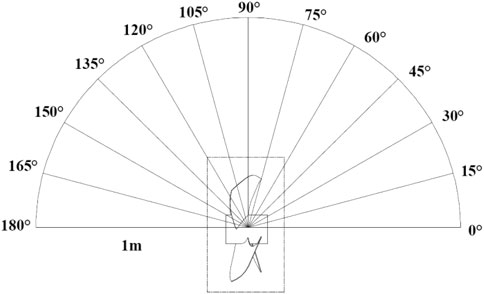
FIGURE 20. Axial flow fan sound pressure level–pointing schematic diagram.
The observed sound pressure values of the measuring points in different directions of the monitoring section were quite different (Figure 21). The sound pressure distribution in the inlet and outlet directions was lower, and the closer to the blade tip, the higher the sound pressure. Comparing the axial fan sound pressure test results before and after optimization, the sound pressure of the axial fan was reduced at 30–75°. Therefore, the optimized blade tip of the axial fan using the Bezier curve had certain noise reduction effects, compared with the original blade tip. This was consistent with the analysis of Figure 19. The noise of the fan is reduced by about 1.1 dB, while the efficiency is increased by 3%, thus reducing the overall energy consumption of the heat pump system.
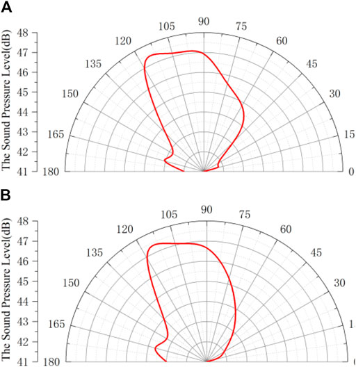
FIGURE 21. Optimized front and rear fan sound pressure level–pointing diagram. (A) Original. (B) Optimized.
1) Through the optimization of the forward-swept blade tip curve, the wind volume increased by 1.78 m3/min and the total pressure efficiency increased by 3.0% at the design flow condition. Improving the total pressure efficiency and flow rate can effectively reduce fan energy consumption and then reduce the energy consumption of the heat pump system.
2) The comparison of the flow field shows that the influence of passage vortexes is weakened in the mainstream direction, so the vortex-induced noise in the mainstream direction should be reduced to some extent. Through further experiments, it is confirmed that the sound pressure level of the optimized axial flow fan decreases at 30–75°, which indicates that the aerodynamic noise of the fan can be reduced by optimizing the forward-swept blade tip curve.
3) In this paper, Bezier function is applied to the parameterized optimization design of axial fan blades, and the ES model is combined with the multi-objective optimization algorithm. The design process of this paper provides a new idea for the optimal design of axial fan and avoids the problem that the traditional agent model is not compatible with the practical engineering problems. The whole optimization design needs fewer design variables, and the optimization process is simple. It provides a way of thinking for the energy-saving design of the heat pump system and has certain engineering application value.
The raw data supporting the conclusions of this article will be made available by the authors, without undue reservation.
KY conceptualized the idea and wrote the article. KY and WJ performed the methodology. SZ and HZ curated the data. SZ prepared the original draft. YH involved in investigation and formal analysis.
This research was supported by the National Natural Science Foundation of China (Grant no. 51706203) and the Natural Science Foundation of Zhejiang Province exploration project (Y, LY20E090004).
The authors declare that the research was conducted in the absence of any commercial or financial relationships that could be construed as a potential conflict of interest.
Thanks are due to ZJUT for providing computing resources and technical support. The authors also appreciate all other scholars for their advice and assistance in improving this article.
Angelini, G., Bonanni, T., Corsini, A., Delibra, G., Tieghi, L., and Volponi, D. (2017). Optimization of an Axial Fan for Air Cooled Condensers. Energ. Proced. 126, 754–761. doi:10.1016/j.egypro.2017.08.236
Cai, L. (1997). Aerodynamic and Acoustic Optimization Design and Experimental Study of Curved Swept Rotor Blades. J. Shanghai Jiao Tong Univ., 031 (002), 81–85.
CONTROLS, REFRIGERATION. ANSI/ASHRAE/IES Standard 90.1-2016 Energy Standard for Buildings except Low-Rise Residential Buildings. Available at webstore.ansi.org/Standards/ASHRAE/ANSIASHRAEIESStandard902016
Della Vecchia, P., Daniele, E., and DʼAmato, E. (2014). An Airfoil Shape Optimization Technique Coupling PARSEC Parameterization and Evolutionary Algorithm. Aerospace Sci. Technol. 32 (1), 103–110. doi:10.1016/j.ast.2013.11.006
Ding, T., Liu, J., and Fang, L. (2019). Optimized Blade Design of Savonius Wind Turbine Based on Multiple Bezier Curves. J. Solar Energ. 038 (004), 959–965.
GB/, T 1236-2017 (2017). Performance Test of Industrial Ventilator with Standardized Air Duct. Beijing: China Standard Press.
Goel, T., Haftka, R. T., Shyy, W., and Queipo, N. V. (2007). Ensemble of Surrogates. Struct. Multidisc Optim 33 (3), 199–216. doi:10.1007/s00158-006-0051-9
Hurault, J., Kouidri, S., Bakir, F., and Rey, R. (2010). Experimental and Numerical Study of the Sweep Effect on Three-Dimensional Flow Downstream of Axial Flow Fans. Flow Meas. Instrum. 21 (2), 155–165. doi:10.1016/j.flowmeasinst.2010.02.003
Jin, R., Chen, W., and Simpson, T. (2000). Comparative Studies of Metamodeling Techniques under Multiple Modeling Criteria. Struct. Multimilitary Optim. 23 (1), 1–13. doi:10.2514/6.2000-4801
Jung, J. H., and Joo, W.-G. (2019). The Effect of the Entrance Hub Geometry on the Efficiency in an Axial Flow Fan. Int. J. Refrig. 101, 90–97. doi:10.1016/j.ijrefrig.2019.02.026
Lim, T.-G., Jung, J. H., Jeon, W.-H., Joo, W.-G., and Minorikawa, G. (2020). Investigation Study on the Flow-Induced Noise by Winglet and Shroud Shape of an Axial Flow Fan at an Outdoor Unit of Air Conditioner. J. Mech. Sci. Technol. 34 (7), 2845–2853. doi:10.1007/s12206-020-0617-2
Lin, Y., Wu, G., and Hu, Y. (2014). Numerical Simulation and Optimization of Internal Flow of Main Feedwater Pump on ACP 1000 THIRD-Generation Nuclear Power Island. Water Pump Technol. 2014 (9), 10–12. doi:10.3969/j.issn.1672-545X.2014.09.004
Liu, L., Hu, L., and Guo, X. (2019). Aerodynamic Optimization Design of Axial Flow Fan Blades with Multiple Working Conditions. J. Eng. Thermophys. 40 (11), 99–106. doi:10.1007/s12206-008-0724-y
Liu, R. (2008). Study on Aerodynamic Calculation of Forward-Curved Forward-Swept Low-Pressure Low-Noise Axial Flow Fans. Northeastern University.
Ravelet, F., Bakir, F., Sarraf, C., and Wang, J. (2018). Experimental Investigation on the Effect of Load Distribution on the Performances of a Counter-rotating Axial-Flow Fan. Exp. Therm. Fluid Sci. 96, 101–110. doi:10.1016/j.expthermflusci.2018.03.004
Schram, C., and Hirschberg, A. (2003). Application of Vortex Sound Theory to Vortex-Pairing Noise: Sensitivity to Errors in Flow Data. J. Sound Vibration 266 (5), 1079–1098. doi:10.1016/S0022-460X(02)01630-9
Srinivas, N., and Deb, K. (1994). Muiltiobjective Optimization Using Nondominated Sorting in Genetic Algorithms. Evol. Comput. 2 (3), 221–248. doi:10.1162/evco.1994.2.3.221
T, J. (2017). The Influence of Serrated Trailing Edge on the Aerodynamic Performance and Internal Flow of Axial Fan. Huazhong University of Science and Technology.
Usman, M., Kliazovich, D., Granelli, F., Bouvry, P., and Castoldi, P. (2017). Energy Efficiency of TCP: An Analytical Model and its Application to Reduce Energy Consumption of the Most Diffused Transport Protocol. Int. J. Commun. Syst. 30 (1), e2934. doi:10.1002/dac.2934
Xie, Y., Xu, M., and Li, K. (2019). Effect of Forward-Swept Angle on the Performance of Axial Flow Cooling Fan for Automotive. J. Northeast. Univ. 40 (6), 862–868.
Xu, L., Li, E., Xu, Y., Mao, N., Shen, X., and Wang, X. (2020). An Experimental Energy Performance Investigation and Economic Analysis on a cascade Heat Pump for High-Temperature Water in Cold Region. Renew. Energ. 152, 674–683. doi:10.1016/j.renene.2020.01.104
Xu, Y., Mao, C., Huang, Y., Shen, X., Xu, X., and Chen, G. (2021). Performance Evaluation and Multi-Objective Optimization of a Low-Temperature CO2 Heat Pump Water Heater Based on Artificial Neural Network and New Economic Analysis. Energy 216 (8), 119232. doi:10.1016/j.energy.2020.119232
Yang, A., and Chen, K. (2002). Influence of Swept Blades on Aerodynamic and Acoustic Characteristics of Rotor of Small Axial Flow Fan. Fluid Machinery 30 (1), 18–20. doi:10.1016/S0731-7085(02)00201-7
Yang, W., and Xiao, R. (2014). Multiobjective Optimization Design of a Pump-Turbine Impeller Based on an Inverse Design Using a Combination Optimization Strategy. J. Fluids Eng. 136 (1), 249–256. doi:10.1115/1.4025454
Ye, P. (2017). Research on Agent Model Technology and its Application in Shape Design of Underwater Glider. Northwestern Polytechnical University.
Zapotecas, M., and Coello, C. (2013). Combining Surrogate Models and Local Search for Dealing with Expensive Multi-Objective Optimization Problems. Evolutionary Computation (CEC). doi:10.1109/CEC.2013.6557879
Zhang, H., Yang, A., and Chen, K. (2019). Relationship between Rotor Blade Sweep Angle and Aerodynamic Performance of Small Axial Flow Fan. J. Power Eng. 2009 (8), 769–772. doi:10.3321/j.issn:1000-6761.2009.08.014
Zhou, S., Li, H., Wang, J., Wang, X., and Ye, J. (2014). Investigation Acoustic Effect of the Convexity-Preserving Axial Flow Fan Based on Bezier Function. Comput. Fluids 102, 85–93. doi:10.1016/j.compfluid.2014.06.019
Zhou, S. (2015). Control and Application of Unsteady Flow Separation in Low-Speed Fans. Huazhong University of Science and Technology.
Zhou, S., Zhou, H., Yang, K., Dong, H., and Gao, Z. (2021). Research on Blade Design Method of Multi-Blade Centrifugal Fan for Building Efficient Ventilation Based on Hicks-Henne Function. Sustainable Energ. Tech. Assessments 43, 100971. doi:10.1016/j.seta.2020.100971
γ Installation angle (°)
b Blade chord length (mm)
r Blade section radius (mm)
L Cover and axial overlap length (mm)
h Blade height (mm)
µl Viscosity coefficient
I Turbulence intensity
DH Outlet diameter (mm)
φ Flow coefficient
ψ Total pressure coefficient
ψS Static pressure coefficient
ηB Total pressure efficiency (%) Original fan total pressure efficiency (%)
QV Fan volume flow (m³/min)
A The first points
B The points at 91 of leaf height
C The points at 83% of leaf height
D The last points
β Angle between A–B and the axis (°)
ωi(x) Corresponding weight factors
qv Fan volume flow (m³/s)
QvB Original fan volume flow (m³/min)
R2 Correlation coefficient
NSGA-II Non-dominated sorting genetic algorithm II
RBF Radial basis function
Opt LHD Optimal Latin hypercube design
ES Ensemble of surrogates
Keywords: forward-swept axial fan, energy conservation design, forward-swept curve parameterization, ensemble of surrogates, multi-objective optimization
Citation: Yang K, Zhou S, Hu Y, Zhou H and Jin W (2021) Energy Efficiency Optimization Design of a Forward-Swept Axial Flow Fan for Heat Pump. Front. Energy Res. 9:700365. doi: 10.3389/fenrg.2021.700365
Received: 26 April 2021; Accepted: 31 May 2021;
Published: 23 June 2021.
Edited by:
Ning Mao, The University of Tokyo, JapanReviewed by:
Jianjun Ye, Huazhong University of Science and Technology, ChinaCopyright © 2021 Yang, Zhou, Hu, Zhou and Jin. This is an open-access article distributed under the terms of the Creative Commons Attribution License (CC BY). The use, distribution or reproduction in other forums is permitted, provided the original author(s) and the copyright owner(s) are credited and that the original publication in this journal is cited, in accordance with accepted academic practice. No use, distribution or reproduction is permitted which does not comply with these terms.
*Correspondence: Shuiqing Zhou, enNxd2g5ODZAMTYzLmNvbQ==
Disclaimer: All claims expressed in this article are solely those of the authors and do not necessarily represent those of their affiliated organizations, or those of the publisher, the editors and the reviewers. Any product that may be evaluated in this article or claim that may be made by its manufacturer is not guaranteed or endorsed by the publisher.
Research integrity at Frontiers
Learn more about the work of our research integrity team to safeguard the quality of each article we publish.