Investigation of Optimal PV Allocation to Minimize System Losses and Improve Voltage Stability for Distribution and Transmission Networks Using MATLAB and DigSilent

Electricity generation from renewable energy sources such as solar energy is an emerging sustainable solution. In the last decade, this sustainable source was not only being used as a source of power generation but also as distributed generation (DG). Many literatures have been published in this field with the objective to minimize losses by optimizing the DG size and location. System losses and voltage profile go hand-in-hand; as a result, when system losses are minimized, eventually the voltage profile improves. With improvement in inverter technologies, PV-DG units do not have to operate at a unity power factor. The majority of proposed algorithms and methods do not consider power factor optimization as a necessary optimization. This article aims to optimize the size, location, and power factor of PV-DG units. The simulations are performed on the IEEE 33 bus radial distribution network and IEEE 14 bus transmission network. The methodologies developed in this article are divided into two sections. The first section aims to optimize the PV-DG size and location. A multi-objective function is developed by using system losses and a voltage deviation index. Genetic algorithm (GA) is used to optimize the multi-objective function. Next, analytical processes are developed for verification. The second section aims to further enhance PV-DG by optimizing the power factor of PV-DG. The simulation is performed for static load in both systems, which are the IEEE 33 bus radial distribution network and IEEE 14 bus transmission network. A mathematical analytical method was developed, and it was found to be sufficient to optimize the power factor of the PV-DG unit. The results obtained show that voltage stability indices help minimize the computation time by determining the optimal locations for DG placement in both networks. In addition, the GA method attained faster convergence than the analytical method and hence is the best optimal sizing for both test systems with minimum computation time. Additionally, the optimization of the power factor for both test systems has demonstrated further improvement in the voltage profile and loss minimization. In conclusion, the proposed methodology has shown promising results for both transmission and distribution networks.

Introduction

The recent development in distributed generation (DG) technologies has started to reshape the conventional power generation and distribution (Keane et al., 2013). DG is categorized into renewable and fossil fuel–based energy sources. Renewable energy sources include solar photovoltaics, wind turbines, biomass generation, and micro-hydro generators. Within the last decade, the worldwide DG capacity has grown significantly. Global investments for DG technologies have increased from $30 billion to $150 billion (Fraser et al., 2002).

The traditional electricity generation is confined to a centralized power generation system. These systems consist of few large-scale power generation units, which are connected to transmission and distribution networks. These networks supply power to the industries and commercial and domestic customers. In a centralized system, a large quantity of power is generated, and the power flow is unidirectional (Di Santo et al., 2015). However, for a DG system, the small-scale generation units are directly connected to the distribution network. These DG units vary from few megawatts to small kilowatts; hence, a bidirectional power flow is achieved (Abapour et al., 2015).

These centralized power generations are usually fossil fuel–based power generations. The production of electricity is one of the major contributors of greenhouse gases. In this sector, CO₂ is considered the major contributor of greenhouse gases emitted in the atmosphere, whereas methane and nitrous oxide are other emitters. These gases cause climate change by trapping heat inside our atmosphere. This increase in the global temperature results in extreme weather, rise in sea level, droughts, and increase in wildfires. Since electricity is the backbone of any growing economy, the energy consumption and demand will increase rapidly. Utilities are tasked with providing reliable and safe power to all the customers within their networks.

In recent years, the development of centralized fossil fuel–based power generations has been stalled due to the depletion of fossil fuels, transmission costs and losses, huge capital cost, and increase in environmental concerns (Zubo et al., 2017). Hence, the demand for greener and more efficient methods of power generation and distribution has increased. Distribution networks with a high penetration of renewable DGs have started to prevail.

Research has revealed that, at any instance, the surface of the earth receives approximately 1.8 × 10¹¹ MW of power from solar radiations. This is more than enough to fulfill the world's power demand (Shah et al., 2015). Solar energy can be harvested in two forms, namely, thermal and photovoltaic. However, the photovoltaic form is the more feasible option (Sangster, 2014).

In addition, with the changes in energy sector regulations, many countries are expected to integrate large-scale renewable generation into the existing grid. For example, in the year 2015, China’s total installed photovoltaic capacity was 43.18 TW. China is becoming the largest photovoltaic generation capacity–installed country in the world (He et al., 2018). As of March 2017, a 12.2 GW solar power capacity was installed by India. The Government of India has announced its mandate to enhance solar energy production to 100 GW by 2022 (Kadam et al., 2017).

Due to the uncontrollable nature of PV-DG, the integration of PV-DG into the existing grid will have several negative impacts on the system if the integration is not done properly. The most common concern is steady state over voltage, effects on the voltage profile, sudden fluctuations of voltage, and the impact on system losses. The voltage profile and system losses are the most important areas that utilities focus as they affect the system reliability (Guerra and Martinez, 2014; Haque and Wolfs, 2016). Furthermore, an increase in penetration would reduce the inertia of the system as power supplied by the conventional generators is decreased. The reduction of active power supplied to the system will have impact on the transient stability of the system (Zainuddin et al., 2018).

System loss minimization has been the major driving force behind most of the research conducted on this field. These research works are based on determining the optimal DG size and location. These optimized DG units could enhance voltage stability and improve the efficiency of the network by loss minimization.

Voltage stability is defined as the ability of a system to maintain acceptable voltage across the system after a disturbance (Bujal et al., 2014). When PV-DG is integrated, the voltage stability of the system is enhanced. As a result, the system’s capacity to transfer more active power is increased. Hence, the installed PV-DG size needs to be controlled. Otherwise, the power generated by PV-DG will exceed the system load resulting in reverse power (Alam et al., 2012). Furthermore, if the increase in the penetration level of PV-DG is not controlled, the system will lose its stability and exceed the boundaries set by the utility.

To ensure a good operational performance of the distribution network, optimal placement and sizing of DGs are critical factors in terms of voltage stability, power quality, profitability, and reliable operational performance of the distribution network. This technical problem of optimal DG placement is in terms with economic maximization, voltage profile improvement, and loss minimization. These are the key components that govern the optimization process.

Several studies have been carried out to achieve an optimum location and size of PV-DG. Different methodologies have been used for this process, and it is based on conventional methods or meta-heuristic algorithms. Conventional methods include analytical analysis, exhaustive analysis, and probabilistic methods, whereas meta-heuristic algorithms include colony optimization, genetic algorithm (GA), and particle swarm optimization (Sadeghian et al., 2017).

The existing literatures on voltage fluctuations are relatively rare, as most of the studies are focused on safety index constraints. Few have highlighted the importance of voltage fluctuations when considering DG capacity (Aziz and Ketjoy, 2017; Liu et al., 2017). These studies still lack an analysis on the relationship between accessible PV-DG capacity and the power factor (Alsafasfeh et al., 2019).

Besides the level of PV penetration and PV size allocation, the power factor of PV-DG is a key aspect that has a direct impact on the voltage profile and system losses. The power factor of the system can be reduced to undesired levels of PF > 0.85 when PV-DG is integrated. Some studies suggest that PV-DG should operate at a power factor more than 0.85 (leading/lagging) when the PV-DG output is more than 10% of the system power (IEEE Standards Coordinating Committee 21 on Fuel Cells Photovoltaic Dispersed Generation and Energy Storage, 2000). Furthermore, most of the research on optimal PV-DG allocation is confined to the distribution network.

Therefore, this article will investigate the optimal location and sizing of the PV-DG unit by using both analytical and meta-heuristic methods. A comparison of both methods will prove the accuracy of the results. The proposed analytical method will consider the voltage stability indices, providing a comprehensive analysis of load flow within the candidate network. In addition, the appropriate power factor for PV-DG penetration is also inspected in this study. IEEE 33 bus distribution network and IEEE 14 bus transmission network systems are selected for simulation and further analysis.

Methodology

A methodology is developed to achieve the three main objectives of this article. Each section is designed to undertake an objective whereas section one highlights the test networks. The methodology is designed for each section to achieve the objective whereas the results can be verified by the next section or within the section. Figure 1 shows the verification process and the methodology outline.

FIGURE 1

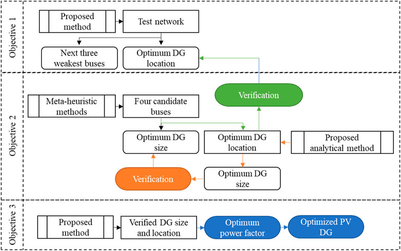
FIGURE 1. Proposed methodology outline.

Test Systems

The test systems selected to simulate the proposed methodology are the IEEE 14 bus system and IEEE 33 bus system which represent the transmission network and distribution network, respectively. The IEEE 14 bus network consists of five generator buses, 11 load buses, and 20 lines (Yadav et al., 2014). For the transmission network, base voltage is 132 kV and base MVA is 100MVA, respectively. Table 1 shows the generator bus voltages used for the IEEE 14 bus system.

TABLE 1

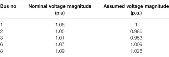
TABLE 1. IEEE 14 bus system.

The standard IEEE 33 bus radial distribution network consists of 33 buses, 32 load branches, and one synchronous generator. Rated voltage for the system is 12.66 KV (Vita, 2017).

Optimum DG Location

To achieve the first objective, two-line stability indices were selected to identify the optimal DG location. These indices are selected after analyzing many literatures. A methodology is developed by using these indices to find the optimal location of the PV-DG unit. This method will identify the weakest bus (optimum DG location). To verify, the next three weakest buses will also be identified. These four buses will be used as candidate buses in the next section.

Line Voltage Stability Indices

The stability of a network can be evaluated by line voltage stability indices. Figure 2 shows the two-bus representation that is used to formulate all line voltage stability indices (VSIs) (Jalboub et al., 2011). The shunt admittance for these representations is ignored since all network lines are simulated for 1 KM in length. Hence, the value for shunt admittance is negligible and can be ignored. All line VSIs are derived on the characteristics of voltage collapse. The main difference between each line VSI is its sensitivity. For example, the FVSI only considers reactive power transfer whereas LQP considers both active and reactive power transfer. The line VSIs selected for this research are briefly described in this section.

FIGURE 2

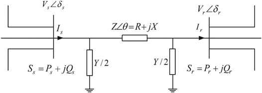
FIGURE 2. Single-line two-bus network.

Fast Voltage Stability Index

The FVSI (Musirin and Abdul Rahman, 2002) is developed based on voltage collapse conditions. For stability operation, the FVSI should be less than unity. The line with the highest FVSI is the most critical line and may lead to system-wide instability. This index is also used to identify the weakest bus. The weakest bus corresponds to the bus with the smallest maximum permissible load.

$\mathit{F}\mathit{V}\mathit{S}{\mathit{I}}_{\mathit{i}\mathit{j}}\mathrm{=}\frac{4{\mathit{Z}}_{\mathit{i}\mathit{j}}^2{\mathit{Q}}_{\mathit{j}}}{{\mathit{V}}_{\mathit{i}}^2\mathit{X}}$

The relative equations are,

Vi = sending end bus voltage magnitude.

Vj = receiving end bus voltage magnitude.

Zij = line impedance.

Rij = line resistance.

Xij = line reactance.

Pi = sending end active power.

Qi = sending end reactive power.

Pj = receiving end active power.

Qj = receiving end reactive power.

Line Stability Factor

LQP is a line stability index developed by Mohamed et al. (1998). This stability index is modeled in a single line network between two nodes to generate the equation. For stable operation, the LQP value should be less than unity. The bus with the lowest LQP value is the most stable bus.

$\mathit{L}\mathit{Q}\mathit{P}=4\left[\frac{{\mathit{X}}_{\mathit{i}\mathit{j}}}{{\mathit{V}}_{\mathit{i}}^2}\right]\left[\frac{{\mathit{X}}_{\mathit{i}\mathit{j}}}{{\mathit{V}}_{\mathit{i}}^2}{\mathit{P}}_{\mathit{i}}^2+{\mathit{Q}}_{\mathit{j}}\right]$

Proposed Analytical Method

To identify the weakest bus, a fixed size of PV-DG at the unity power factor is placed at the receiving end of the line, and load flow is carried. FVSI and LQP values are calculated for all the lines within the networks. An average of these values indicates the stability of the network when PV-DG is installed. The process is then repeated at the sending end of the line. For the FVSI and LQP, the instability point is 1. The smaller the average stability value, it is indicative that the network becomes more stable when PV-DG is placed at that location. Thus, this is the optimum location for PV-DG placement.

To verify the optimum location, the next three weakest lines are selected. For these lines, the same procedure is followed, and an average stability value for the FVSI and LQP is calculated. From the results, three additional candidate buses are selected. These four candidate buses (optimum location and the three additional buses) will be used in the meta-heuristic optimization method to verify the proposed optimal location. Four candidate buses are selected to minimize computation time since it is only being performed to verify the optimum location. Figure 3 shows the flow chart of the proposed method.

FIGURE 3

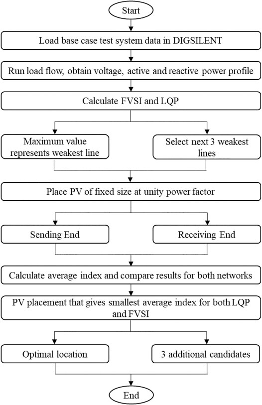
FIGURE 3. Flow chart for the proposed analytical method.

Optimum DG Size

To achieve the second objective, a multi-objective function is formulated to find the optimal size of the PV-DG unit. This multi-objective function is based on active loss reduction and the voltage deviation index of the network. The constraints allocated for the multi-objective function are also defined in this chapter. GA is selected to optimize the multi-objective function. MATLAB is selected as the optimization platform for the algorithm. These optimization solvers provide fast and accurate results with fast convergence time. MATPOWER 7.0 is selected to run Newton-Raphson load flow and to collect required data for the optimization process.

Multi-Objective Function Formulation

To achieve the objective of an optimal PV-DG size, the following multi-objective function (MOF) is formulated by considering real power losses and the voltage deviation index of the network.

$\mathit{M}\mathit{O}\mathit{F}={\mathit{w}}_1\mathit{P}\mathit{L}\mathit{R}+ {\mathit{w}}_2\mathit{V}\mathit{D}\mathit{I}.$

Here, PLR is the active power loss reduction, VDI is the voltage deviation index, and W₁ and W₂ represent the weight of each factor. The summation of all the weights should be equal to 1.

The weights represent the importance of each factor. It may vary from study to study, and this article analyzes different weighs and their impact on the fitness function. Since the minimization of system losses is considered the primary factor for this research, more weightage is given to this parameter. The secondary factor for this study is voltage deviation; hence, the weightage restrictions were allocated accordingly. W1 is restricted between 0.6 and 0.8 whereasW2 is restricted between 0.2 and 0.4. As it was mentioned earlier, this weightage lays more emphasis on real power losses.

Active Power Loss Minimization

Active power loss minimization is one of the main objectives. The active total power loss reduction (PLR) is defined as a ratio between total active power loss after DG installation ($P_{DG{i}_{Loss}}$) and the base total active power loss ($P_{Bas{e}_{Loss}}$); this is represented in the following equation:

$\mathrm{PLR}=\frac{{\mathrm{P}}_{\mathrm{D}\mathrm{G}{\mathrm{i}}_{\mathrm{L}\mathrm{o}\mathrm{s}\mathrm{s}}}}{{\mathrm{P}}_{\mathrm{B}\mathrm{a}\mathrm{s}{\mathrm{e}}_{\mathrm{L}\mathrm{o}\mathrm{s}\mathrm{s}}}}.$

The total active power loss $P_{Loss}$ for both networks is calculated by generating the power flow results. A summation of active power losses of all the branches is calculated. It is written as follows:

${\mathrm{P}}_{loss}={\displaystyle \sum _{k=1}^{N_{br}}{I}_k^2{R}_k}.$

Here, I_k and R_k represent the magnitude of current flow and resistance of the branch number k, respectively, and N_br represents the total number of branches.

Voltage Deviation index

Voltage fluctuations within the set limits are a common occurrence in any distribution network. When networks are less stable these fluctuations can have a direct impact on the system, and sometimes this results in blackouts. Hence, it is advised to minimize any voltage deviation within the system. The voltage deviation index for individual load buses can be identified by finding the square value of the difference between nominal voltage and actual load bus voltage. Performing a summation of these individual voltage deviations will provide the voltage deviation index of the entire network (Le et al., 2007; Uniyal and Kumar, 2018). This is written as follows:

$VDI={\displaystyle \sum }_{k=1}^{N_{br}}{\left[V_n-V_k\right]}^2.$

Here, V_n the nominal voltage 1 p.u., V_k is the voltage at load bus K, and N_br is the number of buses.

Voltage limits

The voltage limits dictate the maximum and minimum limits allowed. This is expressed with the following inequality.

${\mathit{V}}^{\mathit{min}}\le {\mathit{V}}_{\mathit{i}}\le {\mathit{V}}^{\mathit{max}}.$

For this article, the allowed V^max value is 1.05 p.u., whereas the lower bound V_min value is 0.95 p.u.

Generation limits

This constraint limits the size of the PV-DG unit. This is expressed with the following inequality.

$P_{DG}^{\min }\le P_{DGi}\le P_{DG}^{\max }.$

The active power injected by PV-DG should be maintained within the predetermined range. The PV-DG size should not exceed the total load demand (Duong et al., 2019). Hence, the maximum DG capacity is fixed at 100% of the load. For this analysis, maximum PV-DG–injected $P_{DG}^{max}$ value is fixed at 80% of the load demand. Beyond this point, PV-DG will overload. For the minimum PV-DG injection, as mentioned earlier, when DG penetration is low during peak load, the PV inverter does very little to improve the voltage profile of the network. Furthermore, when the penetration percentage is very low, reverse power is also another possibility that would result in excess voltage (Chen et al., 2012). The use of a minimum value also impacts computation time. Hence, for this analysis, the minimum PV-DG penetration $P_{DG}^{min}$ value is fixed at 20% of the total load.

Genetic Algorithm

GA is developed to simulate the mechanics of natural genetics and natural selection based on randomized search algorithms. GA is based on a string structure that is randomized yet structured like evolutionary adaptation for the survival of the fittest. This creates a new string within each generation, using the fittest members from the previous set (Roetzel et al., 2020).

The proposed strategy is expected to determine the optimal PV-DG size for the network. The candidate buses selected from optimal PV-DG placement is incorporated into the fitness function. The proposed voltage limits are incorporated into the network configuration. Generation limits are implemented by setting the lower and upper boundaries of the GA function. The fitness function consists of the proposed multi-objective function (MOF) and the process to find the optimal PV-DG size. MATPOWER 7.0 is used to perform power flow and to extract required data for the analysis.

GA implementation

For multi-objective optimization problems, GA is exceptionally suited as it can scan vast number of datasets and can provide solutions within reasonable time. Hence, GA is widely used for optimization problems. The proposed methodology is implemented via the following steps.

Step 1: Select candidate buses and prepare the test network.

Step 2: Input GA parameters.

Step 3: Initialization creates a random initial population.

Run load flow via MATPOWER 7.0.

Step 4: Evaluate the fitness of each chromosome in initial population using the fitness function (M).

Step 5: While within the generation size,

Select members called parents for mating.

Produce children by crossover or mutation of parents.

New population is generated.

Data string corresponding to the new population is applied to the test network, and load flow is carried out via MATPOWER 7.0.

Fitness of new chromosomes is calculated using the fitness function M.

Number of generations is increased by 1.

Step 6: If stopping criteria are fulfilled, go to Step 7 or go to Step 5.

Step 7: End.

Analytical Method to Find the Optimal Size of PV-DG

The proposed analytical method is developed to verify the results obtained from the meta-heuristic method. This analytical method is developed in MATLAB to minimize system losses by the optimal placement of PV-DG. Since the optimal location of PV-DG is verified, this location is used as the candidate bus. The main concept for this analysis is that with an increase in the DG-PV size, the losses are decreased to their minimum value. But with further increase in the PV-DG size, losses start to increase again (Anwar and Pota, 2011). Hence, the aim of this analysis is to find this optimum PV-DG size. For this analysis, the same generation size constraints of 20–80 percent of the total load demand are used. The following steps describe how the proposed method is designed.

Step 1: Create a vector for PV-DG size constraints (20–80%) with a step size of 0.1. For this analysis, a step size of 0.01 is sufficient. If a smaller step size is used, the number of variables will increase exponentially. Increasing the computation time.

Step 2: Identify the candidate bus for the network, and load the candidate network.

Step 3: Identify the active load demand for the network.

Step 4: Create an empty vector to record the PV-DG size.

Step 5: Create vector k with step size one and with length of PV-DG size constraints vector.

Step 6: For k = 1.

Multiplying the corresponding PV-DG size constraint with the total load demand. This gives the PV-DG size for the analysis.

Install PV-DG of the selected size at the candidate bus.

To activate the generator, the generator status is changed to 1.

To select active power injection, the bus type is changed to 1.

Run load flow by using MATPOWER 7.0.

Record active losses.

Increase the iteration counter k = k+1.

When maximum iterations are achieved, go to Step 7.

Step 7: Select the minimum losses and the corresponding PV-DG size. This is the optimum size of PV-DG.

Step 8: Plot the graph.

Step 9: Stop.

Optimizing the Power Factor

In the previous sections, the PV-DG location and size are optimized at a unity power factor to minimize system losses and to improve the voltage profile. As the network loads are static, a simple analytical method could be used to further optimize the PV-DG unit. The IEEE recommendations for utility interfacing of PV-DG highlights that PV-DG should operate at more than 0.85 of the power factor (leading/lagging) when PV-DG output is more than 10% of the system load (IEEE Standards Coordinating Committee 21 on Fuel Cells Photovoltaics Dispersed Generation and Energy Storage, 2000). Hence, in this simulation, the power factor will fluctuate between 1.00 (unity) and 0.85 lagging. The aim of this section is to investigate the impact of the power factor on system losses and the voltage profile.

Hence, the methodology is built to deliver the optimum power factor for PV connected to the system. For this analysis, the same constraints for the PV-DG size and voltage limits are used. The proposed analytical method relies on the concept of trial and error to find the optimal power factor.

For both networks, the power factor fluctuates between one and 0.85 (lagging). The PV-DG unit is integrated to the network at an optimum location with the optimum penetration percentage and power factor set at unity. The power factor is decreased by 0.1 and load flow is run to obtain the network losses and voltage profile. If losses are decreasing and the constraints are not violated, the process is repeated. Figure 4 shows the flowchart for the optimal PV-DG power factor.

FIGURE 4

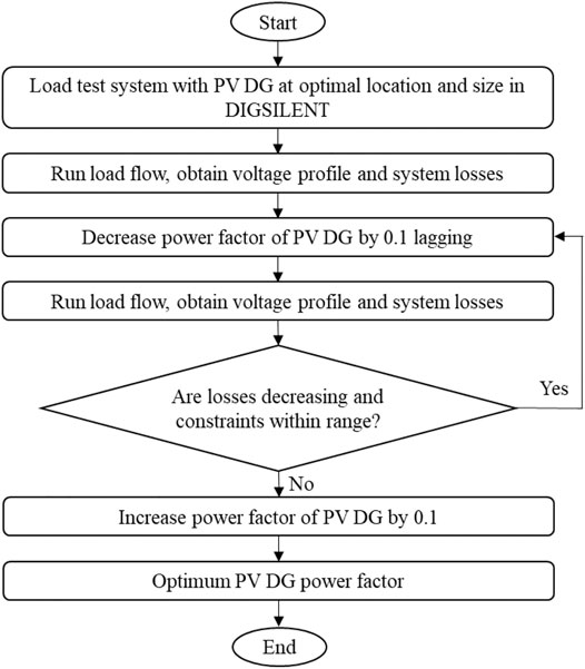
FIGURE 4. Flowchart of optimal PV-DG power factor.

Results

The results are divided into sub-sections; each section fulfils an objective of this article. Comparison has been done to show the reliability and to verify the results. The key components such as reduction in active losses and the improvement of the voltage profile for the proposed methods are compared. The results from this chapter indicate significant improvement in the voltage profile while the system losses are minimized significantly when PV-DG is properly optimized.

Analysis on the Optimal Location

The first step is to establish the base case scenario, and load flow is carried out for both networks without the PV-DG unit. For both networks, the voltage profile and system losses are recorded. The optimal PV-DG location is determined by considering the two voltage stability indices that are selected. From the base case results, line stability for both networks is calculated using the FVSI and LQP index.

Case Study 1: IEEE 14 Bus System

The voltage stability analysis for all lines was analyzed, and the weakest lines were identified. The highest FVSI and LQP value indicates the weakest line. The candidate buses are selected from the 132 KV side of the network. This eliminates buses from one to five. While considering these conditions, the four weakest lines are selected for the analysis.

Both indices clearly identified lines 4–9 as the weakest lines, but to verify this, the next three candidate lines were selected. The results indicate the line 2–3 as the second weakest line, but it is excluded as the line is on the 220 KV side of the network. Hence, based on both stability indices, lines 4–9, 12–13, 13–14, and 5–6 were selected as candidate lines. Buses 4 and 5 were not considered for further analysis, as these buses were located on the 220 KV side of the network.

As these indices could only indicate the weakest line, the proposed methodology provides a solution to identify the candidate bus for PV-DG placement. The proposed analytical method is implemented, and an average value of FVSI and LQP is calculated. The weakest bus is determined by the smallest average FVSI and LQP value. When PV-DG is placed at bus 12, excess voltage is observed, hence eliminating the candidate bus. By analyzing the results, bus 9 is identified as the optimal location. To verify, four candidate buses 6, 9, 13, and 14 were selected as candidate buses for the meta-heuristic method.

Case Study 2: IEEE 33 Bus Distribution Network

The stability of all lines were calculated by using both stability indices. Since the IEEE 33 bus has only one voltage level, no buses were eliminated. The first step is to establish the base case for the network. Newton-Raphson load flow was established, and the voltage profile and system losses were recorded. From this data, the FVSI and LQP value was calculated for the network.

By comparing the stability index of all line four candidates, lines were selected for the analytical process. Lines 5–6 were identified as the weakest lines whereas 27–28, 2–3, and 28–29 were also selected for verification. The proposed analytical method is implemented, and an average value of FVSI and LQP is calculated. The weakest bus is determined by the smallest average FVSI and LQP value.

The analysis of the results indicates bus 3, 6, 27, and 29 as the candidate buses whereas bus 6 displays the weakest characteristics and it is considered the optimum location. To verify this analysis, these four candidate buses will be used for meta-heuristic methods.

Analysis on the Optimal Size

Results of Genetic Algorithm Optimization

According to the methodology, required changes were made to the fitness function. This includes the incorporation of candidate buses and the system constraints. The bus data were modified to allocate the voltage limits whereas the GA solver accommodates the PV-DG size constraint.

Case Study 1: IEEE 14 Bus System

The proposed methodology was implemented in the IEEE 14 bus network. The candidate buses from the previous section (Alam et al., 2012; Bujal et al., 2014; Bujal et al., 2014; Shah et al., 2015; Kadam et al., 2017) were assigned and incorporated to the fitness function in the ascending order. The voltage constraints were limited between 0.95 p.u. and 1.05 p.u. The penetration limits were set between 51.8 and 207.2 MW. GA solver converges at the ninth iteration with the best fitness value of 0.2817. Furthermore, GA requires 22.41 s to complete the optimization.

The two variables of GA solver (X1 and X2) provide the optimal size and location from the candidate buses, respectively.

X1 = Size of PV-DG = 135.5 MW.

X2 = Optimum location = 1.7, this is equal to the second candidate bus for the network.

The second candidate bus corresponds to bus 9, verifying results from the previous section. After the integration of PV-DG of the proposed size at bus 9, significant reduction in active losses was observed. The results indicate active system loss reduction of 53.4%. Figure 5 shows the comparison of system losses between the base case and losses after optimized PV-DG installation.

FIGURE 5

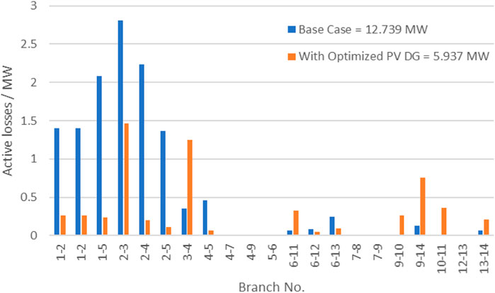
FIGURE 5. System loss comparison for the IEEE 14 bus system.

It was also observed that for some branches active losses were increased; this is due to the increase in current flow within them. Line losses are governed by the equation$P_{loss}=I^{2}R$. Since the size of the conductors remains the same, increase in current flow increases the losses within those lines. But for most of the branches, a significant decrease in active losses was observed.

The lowest voltage is observed at bus 3 with a value of 0.953 p.u. The highest voltage level is observed at bus 8 with a value of 1.028 p.u. While maintaining the voltage limits, the voltage profile for the network improved on average by 0.0094 p.u. Figure 6 shows the comparison of the voltage profile within the base case.

FIGURE 6

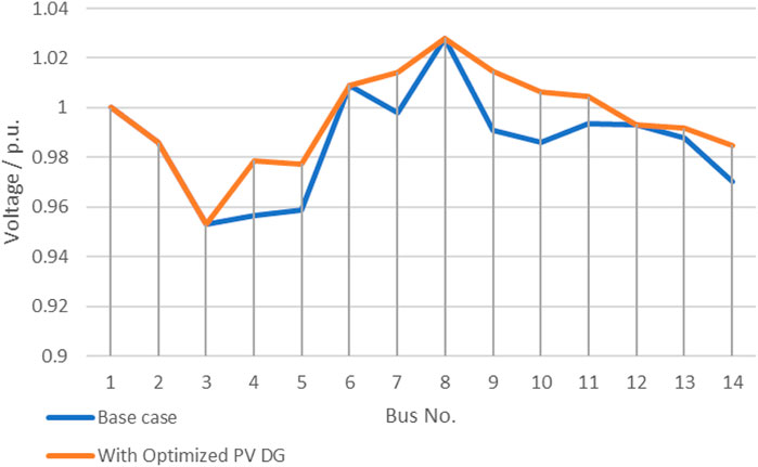
FIGURE 6. Voltage profile comparison for the IEEE 14 bus system.

Case study 2: IEEE 33 bus distribution network

To verify the optimal location proposed in the previous section, four candidate buses (Di Santo et al., 2015; Shah et al., 2015; Duong et al., 2019; Roetzel et al., 2020) were assigned and incorporated to the fitness function in the ascending order. The voltage constraints were limited between 0.95 p.u. and 1.05 p.u. The DG size constraint was implemented at this stage, and limits were set between 0.7 and 3 MW. From the results, it can be highlighted that the GA solver converges at the 10th iteration with the best fitness value of 0.319. Furthermore, GA requires 45.5 s to complete optimization.

The two variables of GA solver (X1 and X2) provide optimal size and location from the candidate buses, respectively.

X1 = Optimal size of PV-DG = 2.675 MW.

X2 = Optimal location = 1.52; this equals to the second candidate bud.

Since the second candidate is bus 6, this verifies the results. When PV-DG of the proposed size was installed at bus 6, significant active loss reduction was observed for all buses within the network. The results indicate an active system loss reduction of 48.8%. Figure 7 shows the comparison of branch losses before and after optimized PV-DG installation.

FIGURE 7

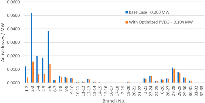
FIGURE 7. System loss comparison for the IEEE 33 bus system.

Since loss reduction and the voltage profile go hand-in-hand, significant improvement in the voltage profile was observed for all buses within the network. The lowest voltage is observed at bus 18 with a value of 0.952 p.u. The highest voltage level is observed at bus 1 with 1 p.u. as the voltage level. This achieves the voltage constraints set for the network. The average voltage profile was improved by a value of 0.027 p.u. Figure 8 shows the comparison of the voltage profile for the network within the base case.

FIGURE 8

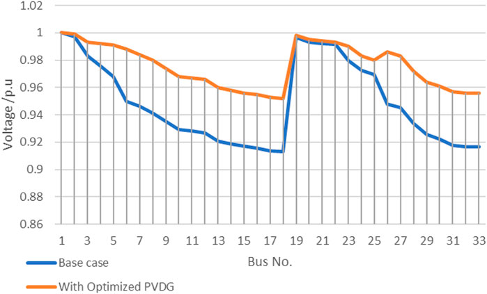
FIGURE 8. Voltage profile comparison for the IEEE 33 bus system.

Results of the Analytical Method

The proposed analytical method was established to verify the optimum PV-DG size for the network. Similar to the meta-heuristic method, DG size constraint was fixed at 20–80% percent of the total load demand, and voltage limits were set at ±5%. At this stage, the optimum location for both networks was verified. Hence, optimum locations will be used to verify the PV-DG size.

Case study 1: IEEE 14 bus system

The proposed methodology was implemented to verify the optimal PV-DG size. The optimum location and network data file were incorporated into the program. The process was started, and the following results were obtained. Figure 9 shows how active loss fluctuates with increase in the PV-DG size.

FIGURE 9

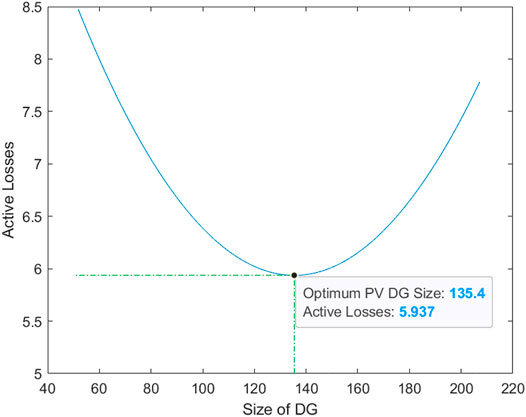
FIGURE 9. Active loss characteristics with PV-DG size variation.

As mentioned earlier, with increase in the PV-DG size, the losses are decreased to their minimum value. But, with further increase in the PV-DG size, the losses start to increase again. The minimum active losses for the network are 5.937 MW, and the corresponding PV-DG size is 135.5 MW. By comparing the results, the optimum PV-DG size can be verified.

Case study 2: IEEE 33 bus system

To verify the optimum PV-DG size, the proposed methodology was implemented. To start the process, the optimum location and network data file were incorporated into the program. Figure 10 shows how active loss fluctuates with increase in the PV-DG size.

FIGURE 10

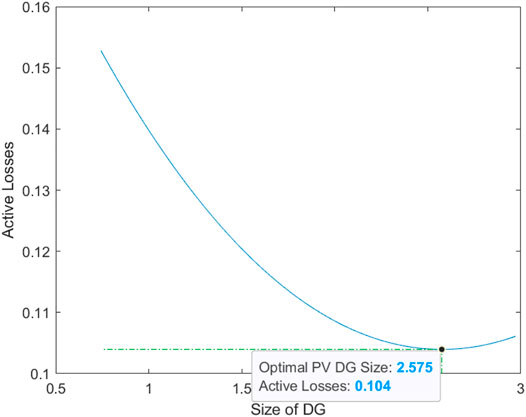
FIGURE 10. Active loss characteristics with PV-DG size variation.

From Figure 10, it can be seen that with the increase in the PV-DG size, losses start to decrease. But beyond 2.574 MW, losses start to increase again. This indicates that 2.5745 MW is the optimum PV-DG size. The results are compared to verify the optimal PV-DG size.

Comparison of Results

Comparison of these results helps us to explore and verify results from each section. Table 2 shows the comparison of optimal size and computation time for the methods explored in this article. The results indicate very similar values for optimal size for both optimization methods.

TABLE 2

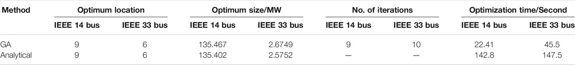
TABLE 2. Comparison of optimal size and computation time for both networks.

An analytical method is used to verify the optimal PV-DG size for the meta-heuristic method. For the IEEE 14 bus system, when the PV-DG size is compared, the difference between the optimal PV-DG size for the meta-heuristic method and analytical method is 0.0605 MW. For the IEEE 33 bus system, when the PV-DG size is compared, the difference between the optimal PV-DG size for the meta-heuristic method and analytical method is 0.0997 MW. The main difference between the meta-heuristic method and the analytical method is computation time. The analytical method requires much longer computation time. Any attempt to make the results more accurate by increasing the step size would further increase computation time with little improvement to the accuracy.

Analysis on optimizing the power factor

After optimizing the PV size and location for both systems to minimize losses and to improve the voltage profile, PV could be optimized further. The power factor should be fluctuated between the unity power factor and 0.85 lagging (IEEE Standards Coordinating Committee 21 on Fuel Cells Photovoltaics Dispersed Generation and Energy Storage, 2000). Hence, the proposed methodology was applied to deliver the optimum power factor for PV connected to the system.

Case Study 1: IEEE 14 Bus System

For the IEEE 14 bus system, when the power factor was minimized to 0.96, the system losses were reduced by 54.3%. Beyond that point, voltage constraints for the system was breached. Figure 11 shows voltage profile improvement when PF was optimized for the IEEE 14 bus system. The results indicate significant voltage profile improvement throughout the network. A maximum voltage of 1.05 was observed at bus 9.

FIGURE 11

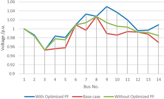
FIGURE 11. Voltage profile of the IEEE 14 bus system after power factor optimization of PV.

Case Study 2: IEEE 33 Bus System

The optimization of the power factor to 0.88 for PV has minimized the system losses from 48.7 to 68.9%. Beyond that point, the PV-DG system overloads. Significant voltage profile improvement was observed for the network with an average improvement of 0.088 p.u. Maximum voltage improvement was observed at bus 18. Figure 12 shows the voltage profile improvement when PF is optimized for the IEEE 33 bus system.

FIGURE 12

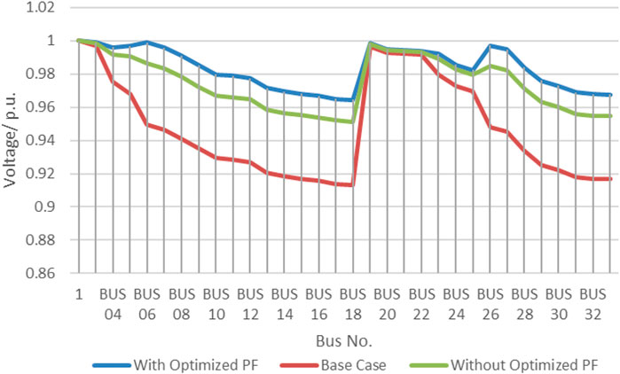
FIGURE 12. Voltage profile of the IEEE 33 bus system after power factor optimization of PV.

Conclusion

Global warming is a disaster that can be mitigated by minimizing fossil fuel usage. One of the main contributors is fossil fuel–based centralized power generation facilities. The use of renewable DGs, such as solar PV, will minimize the power output of these facilities. The introduction of PV-DG units will improve the efficiency of both transmission and distribution networks. This research is designed to minimize system losses and to improve the voltage profile by optimal PV-DG placement. In this article, a static stability model with PV-DG is presented for the IEEE 14 and IEEE 33 bus network. The methodologies presented in this article have been carried out. To find the optimum location of PV-DG, line stability indices were used, and results were verified. To achieve the optimal PV-DG size, a multi-objective function was developed by considering active system losses and voltage deviation indices. The GA and meta-heuristic method were utilized to optimize the multi-objective function. In order to verify the results from the meta-heuristic method, the analytical method was used. The results from GA and analytical method were very similar, verifying the results. It was observed that the active losses for both the IEEE 14 bus system and IEEE 33 bus system were decreased by 53.4 and 48.8%, respectively. Both systems were improved further by optimizing the power factor of PV-DG. Additional active power loss reduction was observed for both the IEEE 14 bus system and IEEE 33 bus system. Active losses were reduced from 53.4 to 54.3% and 48.8–68.9%, respectively. This resulted in considerable voltage profile improvement for both networks while maintaining the constraints proposed in this article. In conclusion, this article has successfully presented that optimal PV-DG can be used in both transmission and distribution networks with satisfactory results. Furthermore, the optimal location and optimal size of PV-DG together with appropriate power factor for PV-DG penetration can significantly reduce the power losses of the system while improving the system voltage profile.

Data Availability Statement

The original contributions presented in the study are included in the article/Supplementary Material; further inquiries can be directed to the corresponding author.

Author Contributions

MR contributed on the simulation work, results, and analysis. RV contributed on the verification of the methodology, results, and analysis. Both authors worked together in writing and editing the manuscript.

Conflict of Interest

The authors declare that the research was conducted in the absence of any commercial or financial relationships that could be construed as a potential conflict of interest.

Publisher’s Note

All claims expressed in this article are solely those of the authors and do not necessarily represent those of their affiliated organizations, or those of the publisher, the editors, and the reviewers. Any product that may be evaluated in this article, or claim that may be made by its manufacturer, is not guaranteed or endorsed by the publisher.

Acknowledgments

The authors would like to thank the Ministry of Higher Education Malaysia for the fundings provided via Fundamental Research Grant 2020 for this research project with code FRGS/1/2020/TK0/UNITEN/02/2 and Universiti Tenaga Nasional for the opportunities given.

References

Abapour, S., Zare, K., and Mohammadi‐Ivatloo, B. (2015). Dynamic Planning of Distributed Generation Units in Active Distribution Network. IET Generation, Transm. Distribution 9 (12), 1455–1463. doi:10.1049/iet-gtd.2014.1143

CrossRef Full Text | Google Scholar

Alam, M. J. E., Muttaqi, K. M., and Sutanto, D. (2012). A Comprehensive Assessment Tool for Solar PV Impacts on Low Voltage Three Phase Distribution Networks. Proc. 2nd Int. Conf. Dev. Renew. Energ. Technol. ICDRET, 221–225.

Google Scholar

Alsafasfeh, Q., Saraereh, O., Khan, I., and Kim, S. (2019). Solar PV Grid Power Flow Analysis. Sustainability 11 (6), 1744. doi:10.3390/su11061744

CrossRef Full Text | Google Scholar

Anwar, A., and Pota, H. R. (2011). “Loss Reduction of Power Distribution Network Using Optimum Size and Location of Distributed Generation,” 2011 21st Australas. Univ. Power Eng. Conf. AUPEC, 2011.

Google Scholar

Aziz, T., and Ketjoy, N. (2017). PV Penetration Limits in Low Voltage Networks and Voltage Variations. IEEE Access 5, 16784–16792. doi:10.1109/ACCESS.2017.2747086

CrossRef Full Text | Google Scholar

Bujal, N. R., Hasan, A. E., and Sulaiman, M. (2014). Analysis of Voltage Stability Problems in Power System. Int. Conf. Eng. Technol. Technopreneuship, Ice2t, 2014, 278–283. doi:10.1109/ICE2T.2014.7006262

CrossRef Full Text | Google Scholar

Chen, P.-C., Salcedo, R., Zhu, Q., de Leon, F., Czarkowski, D., Jiang, Z.-P., et al. (2012). Analysis of Voltage Profile Problems Due to the Penetration of Distributed Generation in Low-Voltage Secondary Distribution Networks. IEEE Trans. Power Deliv. 27 (4), 2020–2028. doi:10.1109/TPWRD.2012.2209684

CrossRef Full Text | Google Scholar

Di Santo, K. G., Kanashiro, E., Di Santo, S. G., and Saidel, M. A. (2015). A Review on Smart Grids and Experiences in Brazil. Renew. Sust. Energ. Rev. 52, 1072–1082. doi:10.1016/j.rser.2015.07.182

CrossRef Full Text | Google Scholar

Duong, M., Pham, T., Nguyen, T., Doan, A., and Tran, H. (2019). Determination of Optimal Location and Sizing of Solar Photovoltaic Distribution Generation Units in Radial Distribution Systems. Energies 12, 174. doi:10.3390/en12010174

CrossRef Full Text | Google Scholar

Guerra, G., and Martinez, J. A. (2014). A Monte Carlo Method for Optimum Placement of Photovoltaic Generation Using a Multicore Computing Environment. IEEE Power Energ. Soc. Gen. Meet. 2014, 1–5. doi:10.1109/PESGM.2014.6939559

CrossRef Full Text | Google Scholar

Fraser, R., Morita, S., and Priddle, R. (2002). Distributed Generation in Liberalised Electricity Markets. Paris: OECD/IEA 2002. doi:10.1787/9789264175976-en

CrossRef Full Text | Google Scholar

Haque, M. M., and Wolfs, P. (2016). A Review of High PV Penetrations in LV Distribution Networks: Present Status, Impacts and Mitigation Measures. Renew. Sust. Energ. Rev. 62, 1195–1208. doi:10.1016/j.rser.2016.04.025

CrossRef Full Text | Google Scholar

He, Y., Pang, Y., Li, X., and Zhang, M. (2018). Dynamic Subsidy Model of Photovoltaic Distributed Generation in China. Renew. Energ. 118, 555–564. doi:10.1016/j.renene.2017.11.042

CrossRef Full Text | Google Scholar

IEEE Standards Coordinating Committee 21 on Fuel Cells Photovoltaics Dispersed Generation and Energy Storage (2000). IEEE Recommended Practice for Utility Interface of Photovoltaic ( PV ) Systems. New York: IEEE/Institute of Electrical and Electronics Engineers Incorporated.

Google Scholar

Kadam, A., Manjunath, M. R., and Bilgundi, S. K. (2017). Optimal Allocation of Solar Photovoltaic Sources in 11kV System for Loss Reduction Using Stress Test Method. Int. Conf. Electr. Electron. Commun. Comput. Technol. Optim. Tech. ICEECCOT 2018, 180–185. doi:10.1109/ICEECCOT.2017.8284661

CrossRef Full Text | Google Scholar

Keane, A., Ochoa, L. F., Borges, C. L. T., Ault, G. W., Alarcon-Rodriguez, A. D., Currie, R. A. F., et al. (2013).State-of-the-art Techniques and Challenges Ahead for Distributed Generation Planning and Optimization. IEEE Trans. Power Syst. 28, 1493–1502. doi:10.1109/TPWRS.2012.2214406

CrossRef Full Text | Google Scholar

Le, A. D., Kashem, M. A., Negnevitsky, M., and Ledwich, G. (2007). Minimising Voltage Deviation in Distribution Feeders by Optimising Size and Location of Distributed Generation. Aust. J. Electr. Elect. Eng. 3 (2), 147–155. doi:10.1080/1448837x.2007.11464155

CrossRef Full Text | Google Scholar

Liu, S., Bi, T., and Liu, Y. (2017). Theoretical Analysis on the Short-Circuit Current of Inverter-Interfaced Renewable Energy Generators with Fault-Ride-Through Capability. Sustainability 10 (1), 44. doi:10.3390/su10010044

CrossRef Full Text | Google Scholar

Jalboub, M., Ihbal, A., Rajamtani, H., Abd-Alhameed, R. A., and Ihbal, A. 2011, Determination of Static Voltage Stability-Margin of the Power System Prior to Voltage Collapse, pp. 1–6. doi:10.1109/ssd.2011.5981420

CrossRef Full Text | Google Scholar

Mohamed, A., Jasmon, G. B., and Yusof, S. (1998). A Static Voltage Collapse Indicator. J. Ind. Technol. 7 (1), 73–85.

Google Scholar

Musirin, I., and Abdul Rahman, T. K. (2002). Novel Fast Voltage Stability index (FVSI) for Voltage Stability Analysis in Power Transmission System. Conf. Res. Dev. Glob. Res. Dev. Electr. Electron. Eng. Scored 2002 - Proc., 265–268. doi:10.1109/SCORED.2002.1033108

CrossRef Full Text | Google Scholar

Roetzel, W., Luo, X., and Chen, D. (2020). Optimal Design of Heat Exchanger Networks. Elsevier, 3.

Google Scholar

Sadeghian, H., Athari, M. H., and Wang, Z. (2017). Optimized Solar Photovoltaic Generation in a Real Local Distribution Network. IEEE Power Energ. Soc. Innov. Smart Grid Technol. Conf. ISGT, 2017. doi:10.1109/ISGT.2017.8086067

CrossRef Full Text | Google Scholar

Sangster, A. J. (2014). Solar Photovoltaics. Green. Energ. Technol. 194 (4/5), 145–172. doi:10.1007/978-3-319-08512-8_7

CrossRef Full Text | Google Scholar

Shah, R., Mithulananthan, N., Bansal, R. C., and Ramachandaramurthy, V. K. (2015). A Review of Key Power System Stability Challenges for Large-Scale PV Integration. Renew. Sust. Energ. Rev. 41, 1423–1436. doi:10.1016/j.rser.2014.09.027

CrossRef Full Text | Google Scholar

Uniyal, A., and Kumar, A. (2018). Optimal Distributed Generation Placement with Multiple Objectives Considering Probabilistic Load. Proced. Comp. Sci. 125, 382–388. doi:10.1016/j.procs.2017.12.050

CrossRef Full Text | Google Scholar

Vita, V. (2017). Development of a Decision-Making Algorithm for the Optimum Size and Placement of Distributed Generation Units in Distribution Networks. Energies 10 (9), 1433. doi:10.3390/en10091433

CrossRef Full Text | Google Scholar

Yadav, S., Mandal, R. K., and Choudhary, G. K. (2014). Determination of Appropriate Location of Superconducting Fault Current Limiter in the Smart Grid. Int. Conf. Smart Electr. Grid, ISEG, 1–9. doi:10.1109/ISEG.2014.7005580

CrossRef Full Text | Google Scholar

Zainuddin, M., Sarjiya, T. P., Handayani, W., Sunanda, , and Surusa, F. E. P. (2018). Transient Stability Assessment of Large Scale Grid-Connected Photovoltaic on Transmission System. 2018 2nd International Conference on Green Energy and Applications (ICGEA), 113–118. doi:10.1109/ICGEA.2018.83562702018

CrossRef Full Text | Google Scholar

Zubo, R. H. A., Mokryani, G., Rajamani, H.-S., Aghaei, J., Niknam, T., and Pillai, P. (2017). Operation and Planning of Distribution Networks with Integration of Renewable Distributed Generators Considering Uncertainties: A Review. Renew. Sust. Energ. Rev. 72 (May), 1177–1198. doi:10.1016/j.rser.2016.10.036

CrossRef Full Text | Google Scholar