Kalman Filter Photovoltaic Power Prediction Model Based on Forecasting Experience

A Kalman filter photovoltaic (PV) power prediction model based on forecasting experience is proposed to solve the problem that the accuracy of the prediction method based on historical experience is reduced under anomalous situations. This study uses the hourly solar irradiance forecasting model, numerical weather prediction (NWP) data, and the photoelectric conversion model to calculate the ground irradiance and PV power generation, which are used as the forecasting experience data. The dynamic equation of the Kalman filter model is obtained by fitting the forecasting data to make the prediction model with the future situation information properties while solving the modeling difficulties caused by the transcendental equation characteristic of the photoelectric conversion model. In the iterative process of the Kalman filter algorithm, the measured power is used to correct the prediction error and significantly limit the error variability so as to realize the ultra-short-term accurate prediction of PV power and ultimately improve the management of PV energy storage power stations. The comparative analysis through DKASC data simulation verifies that the results show that the proposed model is effective and can achieve better results in predictive accuracy.

Introduction

In recent years, fossil energy is becoming increasingly depleted worldwide. In order to alleviate the energy crisis and reduce environmental pollution, solar energy has been widely developed and applied as a green and environmentally friendly renewable energy source. According to the International Renewable Energy Agency (IRENA), the global cumulative installed PV capacity maintained a steady upward trend from 2010 to 2019, and the total installed capacity reached 584,842 MW by 2019 (IRENA, 2020). PV power generation is cyclical and randomly fluctuating due to weather factors, which makes it difficult for PV power generation to be connected to the grid effectively and reduces the PV power generation consumption level (Salim et al., 2018). In addition, the random fluctuation of PV power generation also affects the management level of battery energy storage power stations, making them more costly to operate. The ultra-short-term accurate prediction of PV power generation is an important prerequisite to solve the effective grid connection of PV power generation and improve the management level of energy storage power stations (Bortolini et al., 2014).

In the existing literature related to forecasting, the short-term power forecasting method for PV power generation can be roughly split into the following three categories: physical, statistical, and machine learning methods (Zhou et al., 2020). In the physical, it is implemented by using physical models such as a solar irradiance equation and PV module operation equation and combined with NWP data; instead, the statistical method is based on statistical modeling of historical weather data and PV power data to find out the regularity of historical data for prediction; the machine learning method, as a branch of artificial intelligence, can learn directly from datasets to construct a nonlinear mapping between input and output data to achieve PV power prediction without explicit programming.

Atique et al. (2019) used ARIMA time series model to forecast the total daily solar power generation by studying the seasonal and nonseasonal variations of the total daily solar panel generation and converted the time series data into stationary data. Bacher et al. (2009) entered historical power output and predicted irradiance into an autoregressive model with exogenous inputs for a power output prediction up to 6 h in advance. Hassanzadeh et al. (2010) indirectly forecasted PV power generation by predicting solar irradiance through the Kalman filter algorithm and then used the least square method to forecast PV power generation. Scolari and Sossan, (2017) used an extended Kalman filter (EKF) algorithm to predict PV power by subjecting the PV panel mathematical model to Taylor expansion as an observation matrix. However, the PV panel mathematical model is a transcendental equation, and it is difficult to obtain a system state space model.

Sharadga et al. (2019) evaluated the performance of different neural networks and statistical models and compared the prediction of PV power generation in the time series prediction of large PV power plants. Zhang et al. (2015) proposed a method for PV power generation forecasting based on similar days, consisting of an SDD engine and a prediction engine. And it could achieve high accuracy. Wang et al. (2019) proposed a convolutional neural network, a long- and short-term memory network and a hybrid model based on the convolutional neural network and a long- and short-term memory network model to forecast PV power generation and compared the models. Khan et al. (2017) used the back-propagation (BP) neural network model to predict PV output power in haze weather and regarded solar radiation intensity, wind speed, temperature, humidity, and atmospheric mass index as input attributes. Meng et al. (2018) presented a hybrid model combining the back-propagation neural network (BPNN) and GA to forecast PV power generation. Dong et al. (2020) used a convolutional neural network framework to predict solar irradiance, where the GA and the particle swarm optimization were used to optimize the relevant parameters. However, in traditional ANNs, a large number of parameters need to be optimized by GA, which would greatly increase the computational complexity. And the method based on the BP neural network has a good approximation ability, but it is easy to fall into the misunderstanding of local minimum (Liu et al., 2017).

The literature analysis reveals that the existing forecasting methods are based on historical experience for power prediction. Such forecasting methods require a large amount of historical data and computational effort. In addition, atmospheric pollution and the anomalies of the atmospheric environment caused by El Nino leave the historical database with insufficient experience, which can seriously affect the accuracy of PV power prediction. Furthermore, the NWP service provided by the World Meteorological Organization (WMO) is becoming increasingly sophisticated. We can easily query the detailed weather conditions such as temperature, cloud cover, dew point, humidity, visibility, and other forecasting data for the next 24–72 h by using the mobile APP service (Qing and Niu, 2018). Different from the existing methods, this article proposes a PV power forecasting method based on forecasting experience, which uses forecasting experience data to establish a model to solve the problem of insufficient historical experience due to sudden weather change situations. The predictive architecture is shown in Figure 1.

FIGURE 1

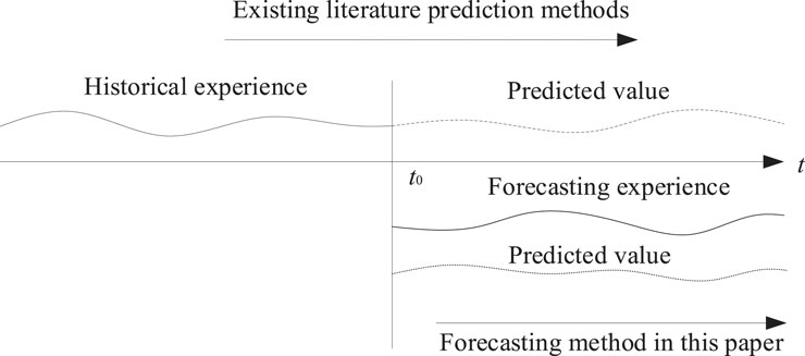
FIGURE 1. Predictive architecture schematic.

This article presents a Kalman filter PV power prediction model based on the hourly solar irradiance model and NWP data. The specific contents of this article are organized as follows: Introduction analyzes the relevant literature and then proposes the model prediction structure; Hourly Forecast of Solar Irradiance calculates the irradiance forecasting experience data based on the hourly solar irradiance forecasting model, considering cloud cover and geographic position; Photoelectric Conversion Model calculates the power forecasting experience data based on the photoelectric conversion model; Kalman Filter Prediction Model Based on Forecasting Experience establishes a Kalman filter PV power prediction model based on the previous forecasting experience data; Simulation and Result Analysis presents the simulation results; Finally, Conclusions concludes.

Hourly Forecast of Solar Irradiance

The solar irradiance received on the surface of the earth is periodic and nonstationary due to the influence of the Earth’s rotation and revolution. In addition, the cloud movement causes the ground solar irradiance to be random and uncertain. In this section, considering the factors of atmospheric attenuation and cloud cover, the irradiance of the ground is calculated based on the hourly solar irradiance model.

Astronomical Irradiance

According to Obukhov et al. (2018), the daily average I_ON of extra-atmospheric solar radiation on the horizontal surface is calculated as follows:

$I_{\mathrm{ON}}=\frac{24}{\pi }\cdot I_{\mathrm{SC}}\cdot \left(\mathrm{1}+\mathrm{0}\mathrm{.033}\cdot \cos \frac{360\cdot N}{365}\right)\cdot \left(\cos \mathit{\phi }\cdot \cos \delta \cdot \sin w_{\text{s}}+\sin \mathit{\phi }\cdot \sin \delta \right),(1)$

where I_SC = 1367W/m² is the solar constant; N is the day number, such that N = 1 on 1st January; φ is the latitude of the receiving surface locality; δ is the solar declination angle; and w_s is the solar hour angle.

The declination angle is obtained as follows:

$\delta =\mathrm{23}\mathrm{.45}\cdot \sin \left(360\cdot \frac{284+N}{365}\right).(2)$

Sunshine Time Correction

The PV power stations are usually located on the slope with a certain inclination angle rather than a horizontal plane. Then, the sunrise time and sunset time are determined when the sunlight is parallel to the module surface, using the PV module surface as a reference.

The sunrise and sunset hour angles of horizontal can be obtained as follows:

$w_0=\arccos \left(-\tan \delta \cdot \tan \phi \right).(3)$

The sunrise and sunset hour angles of atmosphere refraction can be obtained as follows:

$w_{\mathrm{s}}=\arccos \left(\frac{\sin h_0-\sin \phi \cdot \sin \delta }{cos\phi \cdot \cos \delta }\right),(4)$

where h₀ = −0.8333°.

The sunrise and sunset hour angle differences caused by the atmospheric refraction can be obtained as follows:

$△w=w_{\text{s}}-w_0.(5)$

For non-horizontal planes, the sunrise and sunset hour angle correction caused by atmospheric refraction is given as follows:

$w_{\mathrm{up}}=w{\mathrm{\prime }}_{\mathrm{up}}-△w,(6)$

$w_{\mathrm{down}}=w{\mathrm{\prime }}_{down}+△w,(7)$

where $w_{\text{up}}^{\text{′}}$ and $w_{\text{down}}^{\text{′}}$ is the sunrise and sunset hour angles toward the inclined plane in any direction, which can be calculated by Bingzhong (1999).

Then the sunrise and sunset time correction based on an inclined plane is as follows Eqs 8, 9:

$t_{\text{up}}=12+\frac{w_{\text{up}}}{15},(8)$

$t_{\text{down}}=12+\frac{w_{\text{down}}}{15}.(9)$

The astronomical irradiance of PV power station can be determined by Eqs 1, 2, 4. And the sunshine time is ultimately determined by Eqs 8, 9.

Irradiance Attenuation

The extra-atmospheric solar radiation reaches the ground after being attenuated by the atmosphere and cloud cover. Considering the atmospheric mass and transparency, the total solar radiation can be decomposed into direct radiation and scattered radiation (Chicco et al., 2016). In addition, due to the tilt angle of the PV array, the solar irradiance I_S received by the PV array surface can be calculated as follows:

Direct radiation on an inclined surface can be obtained as follows:

$I_D=I_{ON}\cdot P^m\cdot \cos i.(10)$

Scattered radiation on inclined surface can be obtained as follows:

$I_d=\frac{1}{2}\cdot I_{ON}\cdot \sin \alpha \cdot \frac{1-P^m}{1-1.4\cdot \ln P}{\cos }^2\frac{\theta }{2}.(11)$

Total solar radiation can be obtained as follows:

$I_S=I_D+I_d.(12)$

Here, p is the atmospheric transmittance; m is the air quality; i is the solar incidence angle; α is the solar elevation angle; and θ is the tilt angle of PV array.

After atmospheric attenuation, the total solar radiation is absorbed, scattered, and reflected by clouds, and only a fraction of it will reach the ground. Mobile cloud shading is the main cause of irradiance fluctuation. Thus, according to NWP data of the cloud, we can use the cloud cover coefficient method to calculate solar irradiance for cloudy and other conditions (Qishen, 1986). The cloud cover coefficients are shown in Table 1.

TABLE 1

TABLE 1. Cloud cover coefficient.

The solar irradiance received by the surface of the PV array under cloud shelter can be obtained as follows:

$\{\begin{array}{l}{\mathit{I}}_{\mathrm{scs}}=I_{\mathrm{s}}\cdot \mathrm{d}\hfill \\ \mathrm{d}=\mathrm{c}+\mathrm{b}\cdot \mathrm{CC}+\mathrm{a}\cdot \mathrm{C}{\mathrm{C}}^2\hfill \end{array}(13)$

where I_scs is the solar irradiance received by the surface of the PV array under cloud shelter; d is the weakening coefficient of the cloud to the solar radiation; and CC is the cloud cover; if CC ≤ 2, the value of d is 1, if CC ≥ 3, we can calculate the value of d according to Eq. 13. c, b, and a are empirical coefficients, as shown in Table 2 (NBSLD, 1974).

TABLE 2

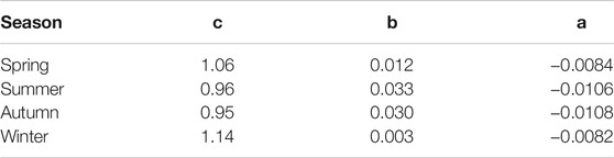
TABLE 2. Empirical coefficients value of c, b, and a.

This study uses the data of the Desert Knowledge Australia Solar Centre (DKASC) (DKASC, 2019). The DKASC is located in central Australia (23°42′0″S, 133°52′12″E). We use the data from April 20, 2019 until April 22, 2019 as our forecasting days and then the hourly irradiance on the PV array surface determined by the above model is shown in Figure 2.

FIGURE 2

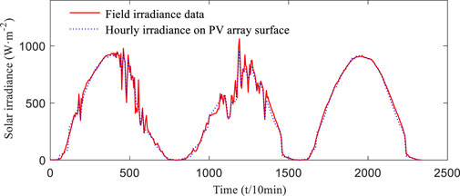
FIGURE 2. Hourly irradiance on PV array surface in forecasting days.

Photoelectric Conversion Model

According to the irradiance in forecasting days, the power generation of the PV power station can be calculated by the solar cell model. The PV conversion model used for simulation in this study uses Luft et al.’s TRW model (Desoto et al., 2006) which is given as follows:

$I=I_{\text{sc}}\left[1-k_2\left(\exp \left(\frac{V}{k_1\cdot V_{\text{oc}}}\right)-1\right)\right],(14)$

in which

$k_1=\frac{\left(\frac{V_{\text{mp}}}{V_{\text{oc}}}-1\right)}{\ln \left(1-\frac{I_{\text{mp}}}{I_{\text{sc}}}\right)},(15)$

$k_2=\left(1-\frac{I_{\text{mp}}}{I_{\text{sc}}}\right)\exp \left(-\frac{V_{\text{mp}}}{k_1\cdot V_{\text{oc}}}\right).(16)$

The power output of the PV panel is calculated as follows:

$P\left(V\right)=V\cdot I_{\text{sc}}\left\{1-k_2\left[\exp \left(\frac{V}{k_1\cdot V_{\text{oc}}}\right)-1\right]\right\}.(17)$

Considering the solar radiation variation, array temperature, and load affecting the efficiency of PV cells, this study regards I_scref, V_ocref, V_mpref, and I_mpref as PV parameters under standard conditions (G_ref = 1000 W/m², T_ref = 25°C). The related parameters I_sc, V_oc, V_mp, and I_mp can be obtained by the following formula (Xu et al., 2016):

$I_{\mathrm{sc}}=I_{\mathrm{scref}}\cdot \frac{G}{G_{\mathrm{ref}}}\left(1+\mathrm{a}\cdot \Delta T\right),(18)$

$V_{\mathrm{oc}}=V_{\mathrm{ocref}}\cdot \ln \left(\mathrm{e}+\mathrm{b}\cdot \Delta G\right)\left(1-\mathrm{c}\cdot \Delta T\right),(19)$

$I_{\mathrm{mp}}=I_{\mathrm{mpref}}\cdot \frac{G}{G_{\mathrm{ref}}}\left(1+\mathrm{a}\cdot \Delta T\right),(20)$

$V_{\mathrm{mp}}=V_{\mathrm{mpref}}\cdot \ln \left(\mathrm{e}+\mathrm{b}\cdot \Delta G\right)\left(1-\mathrm{c}\cdot \Delta T\right).(21)$

Here, $\Delta$G =(G/G_ref−1);$\Delta$T =(T−T_ref); and e is natural logarithm; The compensation coefficients a, b, and c are constant, which can be fitted according to a large amount of empirical data, and the typical value is a = 0.025/°C, b = 0.5/(W/m²), and c = 0.00288/°C (Singer et al., 1984).

The equipment configuration parameters of the DKASC PV system (Alice Springs) are shown in Table 3. And the NWP temperature data in forecasting days are shown in Figure 3. Using the irradiance data in Figure 2 and the temperature data in Figure 3 as inputs, the output power curve of DKASC in forecasting days is calculated by the photoelectric conversion model, as shown in Figure 4.

TABLE 3

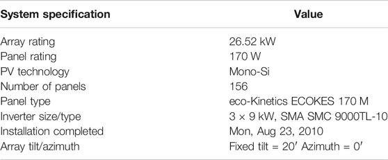
TABLE 3. Equipment configuration parameters of the DKASC PV system.

FIGURE 3

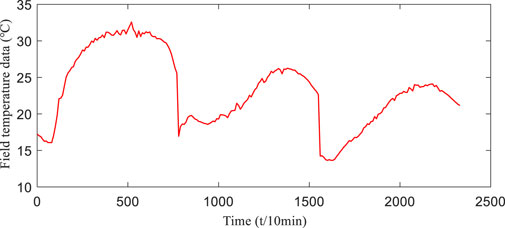
FIGURE 3. NWP temperature data in forecasting days.

FIGURE 4

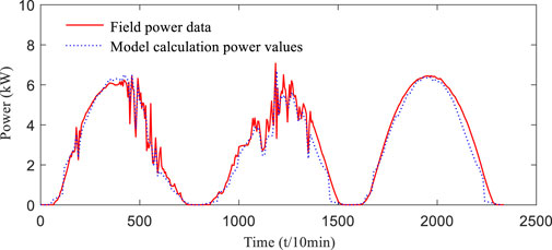
FIGURE 4. Model calculation power values in forecasting days.

The aforementioned model forecasts the power value of PV power generation by physical methods. However, it lacks the dynamic correction process of the prediction results, and the prediction accuracy is insufficient. The forecasting method proposed in this article takes the prediction results of this stage as the forecasting experience and establishes the Kalman filter PV power prediction model.

Kalman Filter Prediction Model Based on Forecasting Experience

The key of the Kalman filter algorithm is to establish the system dynamic equation, and the empirical information of the PV power prediction system is contained in the dynamic equation. However, due to the transcending equations characteristic of the PV cell’s physical model, it is difficult to establish the analytical expressions of the dynamic equations required for the prediction model. Different from the existing literature based on historical experience, this study considers solar irradiance as the system state variable and PV power generation as the system observation, uses the aforementioned model results as forecasting experience data to fit the observation equation of the prediction model, and then introduces the excitation noise as the control equation input quantity to determine the system differential control equation. By iterative recursion of the Kalman filter, the predicted power value at the next time is dynamically corrected by the measurement power value at the previous time, which improves the prediction accuracy of PV power. The framework established by the Kalman filter PV power dynamic equation based on forecasting experience is shown in Figure 5.

FIGURE 5

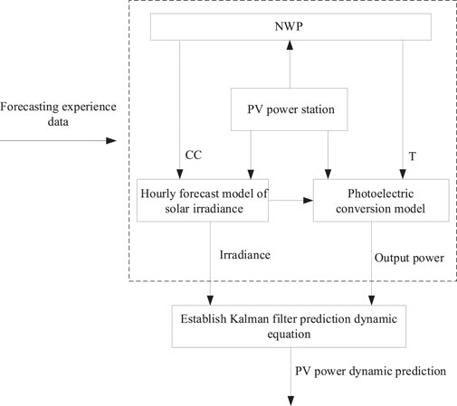
FIGURE 5. Framework established by the Kalman filter dynamic equation.

The Dynamic Model of PV Power Prediction System

The Kalman filter algorithm state equation and observation equation can be obtained as follows:

$\begin{array}{l}{\mathit{x}}_{\mathit{t}}=\mathit{A}\cdot {\mathit{x}}_{\mathit{t-1}}+{\mathit{Q}}_{\mathit{t}}\\ {\mathit{y}}_{\mathit{t}}=\mathit{H}\cdot {\mathit{x}}_{\mathit{t}}+{\mathit{R}}_{\mathit{t}}\end{array}(22)$

Here, x_t is the estimated target state vector at time t; y_t is the estimated target observation vector at time t; A is the state transition matrix; H is the observation matrix; Q_t is the system excitation noise covariance matrix; and R_t is the system observation noise covariance matrix.

Regarding I_s as the system state variable, p as the system observation, and then using the least squares method polynomial fitting to obtain the model’s observation vector y_t expression which is denoted as follows:

${\mathit{y}}_{\mathit{t}}={\mathit{x}}_{\mathit{0,t}}+{\mathit{x}}_{\mathit{1,t}}\cdot m_t+{\mathit{x}}_{\mathit{2,t}}\cdot m_t^2+\cdots +{\mathit{x}}_{\mathit{n,t}}\cdot m_t^n+{\mathit{R}}_{\mathit{t}}.(23)$

Here, x_n,t is the system state variable, solar irradiance, and m_t is the polynomial coefficient that forms the observation matrix H_t.

Considering the data nonlinearity and fitting accuracy, the third-order polynomial is selected for fitting, which can effectively reduce the system bias and fitting time. Using the data in Figures 2, 3 as the forecasting experience data, the fitting curve is shown in Figure 6.

FIGURE 6

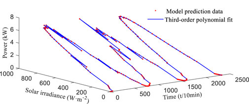
FIGURE 6. Observation equation curve.

The state space equation of the PV power prediction system can be expressed as follows:

${\mathit{x}}_{\mathit{t}}=\mathit{A}\cdot {\mathit{x}}_{\mathit{t-1}}+{\mathit{Q}}_{\mathit{t}}.(24)$

Here, the state transition matrix A coincides with the identity matrix I, and Q_t and R_t are the model error and the instrument error, respectively, which should be estimated by utilizing the last seven values of the model window data, the number that sensitivity tests proved as optimal (Galanis et al., 2017).

${\mathit{Q}}_{{\mathit{t}}_{\mathit{i}}}=\frac{1}{6}\cdot {\displaystyle \sum _{i=0}^6{\left[\left(x_{t_i+1}-x_{t_i}\right)-\left(\frac{{\displaystyle {\sum }_{i=0}^6\left(x_{t_i+1}-x_{t_i}\right)}}{7}\right)\right]}^2}(25)$

${\mathit{R}}_{{\mathit{t}}_{\mathit{i}}}=\frac{1}{6}\cdot {\displaystyle \sum _{i=0}^6{\left(\left(y_{t_i}-H_{t_i}{x}_{t_i}\right)-\left[\frac{{\displaystyle {\sum }_{i=0}^6\left(y_{t_i}-H_{t_i}{x}_{t_i}\right)}}{7}\right]\right)}^2}(26)$

In the method proposed in this article, the Kalman filter is a dynamic estimation process. The forecasting window is updated in real time based on the NWP data of the cloud to achieve the goal of sampling and fitting prediction each hour, making the Kalman filter algorithm meet the criteria of being dynamic and flexible yet reliable.

Dynamic Correction Process

The initial value of state vector x_t which is denoted as follows:

${\mathit{x}}_{\mathit{t}\text{/}\mathrm{t-1}}=\mathit{A}\cdot {\mathit{x}}_{\mathit{t}-1}.(27)$

The state covariance matrix as follows:

${\mathit{P}}_{\mathit{t}/t-1}=\mathit{A}\cdot {\mathit{P}}_{t-1}\cdot {\mathit{A}}^{\mathit{T}}+{\mathit{Q}}_{t-1}.(28)$

After the observation value y_t is determined, the estimated value of state vector x at time t as follows:

${\widehat{x}}_t={\mathit{x}}_{\mathit{t/t-1}}+{\mathit{K}}_t\cdot \left({\mathit{y}}_{\mathit{t}}-{\mathit{H}}_{\mathit{t}}\cdot {\mathit{x}}_{\mathit{t/t-1}}\right)(29)$

K_t is the Kalman gain, which serves to ensure that the Kalman filter algorithm adapts to any dynamic process, and can be determined by the following formula:

${\mathit{K}}_{\mathit{t}}={\mathit{P}}_{\mathit{t}/\mathit{t}-1}\cdot {\mathit{H}}_{\mathit{t}}^{\mathit{T}}{\left({\mathit{H}}_{\mathit{t}}\cdot {\mathit{P}}_{\mathit{t}/t-1}\cdot {\mathit{H}}_{\mathit{t}}^{\mathit{T}}+{\mathit{R}}_{\mathit{t}}\right)}^{-1}.(30)$

After iteration, the state covariance matrix as follows:

${\mathit{P}}_{\text{t}}=\left(I-{\mathit{K}}_{\mathrm{t}}\cdot {\mathit{H}}_{\mathrm{t}}\right)\cdot {\mathit{P}}_{\mathrm{t/t-1}}.(31)$

The recursive nature of the state equation and the linear unbiased least mean square estimation criterion are used to make the best estimate of the state variables of the Kalman filter. And then by using the state equation of signal and noise, the estimated values and observed values at the previous time and the current time are compared to update the state variables and realize the estimation of the state variables. The Kalman filter algorithm is recursive in the order of “prediction-measurement-correction,” based on a series of observations of random states to make quantitative inferences, and the minimum mean square error to make the estimated value more accurately close to the true value. The algorithm flow is shown in Figure 7.

FIGURE 7

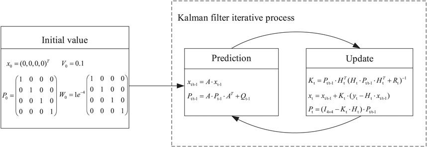
FIGURE 7. Kalman filter PV power prediction flow.

Simulation and Result Analysis

We use the data from April 20, 2019 until April 22, 2019 for simulation verification. Observation Eq. 23 is determined by fitting the forecasting experience data, which are hourly irradiance on the PV array surface in Figure 2 and the model calculation power values in Figure 3 in forecasting days. The ultra-short-term prediction of PV power is achieved by the dynamic correction process of the Kalman filter prediction model. And the forecasting window can be adjusted according to the NWP data.

The error evaluation of the system uses absolute percentage error as follows:

$E_{\text{ape}}=\left|\frac{y_{pi}-y_{qi}}{y_{qi}}\right|\times 100\%.(32)$

Here, y_pi is the predicted value and y_qi is the actual value.

The Kalman filter PV power prediction curve is shown in Figure 8, and the error curve is shown in Figure 9. To facilitate comparative analysis, the predicted data of the Kalman filter model based on forecasting experience and the predicted data of the Kalman filter model based on historical experience are given in the figure (Ying and Tianyang, 2021). The sampling period of DKASC field output power data is 5 min. In practice, considering the NWP time scale and leaving sufficient preparation margin for the ultra-short-term prediction of PV power, the data sampling period in this simulation is 10 min. The horizontal coordinate of the graph indicates the time, and the data of the forecasting days are used and expressed as continuous values.

FIGURE 8

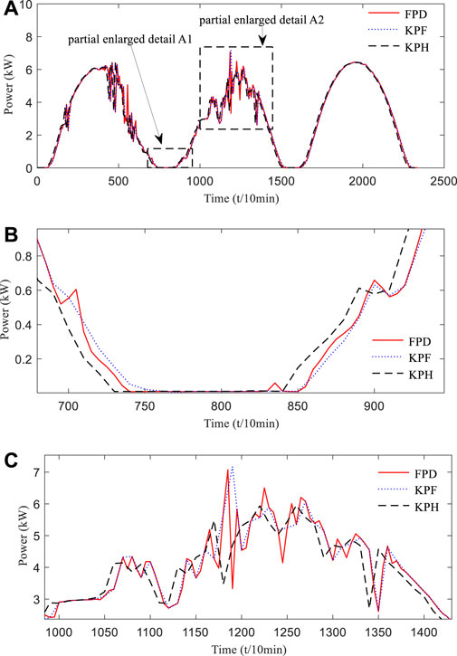
FIGURE 8. Kalman filter model PV power prediction curve. (A) Photovoltaic power prediction curve in forecasting days; (B) Photovoltaic power prediction curve in insufficient illumination; (C) Photovoltaic power prediction curve in sufficient illumination.

FIGURE 9

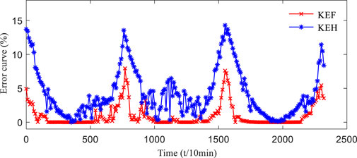
FIGURE 9. Kalman filter model PV power prediction error curve.

In order to effectively verify the effectiveness of the prediction model established in this article, the DKASC data selected in the first 2 days of weather conditions change significantly are used to simulate the historical experience of insufficient, anomalous output power situations; the third-day weather conditions are more normal and used to simulate the historical experience of sufficient, normal output power situations. As shown in Figure 8, the predicted power curve of the Kalman filter model based on forecasting experience is in good agreement with the actual power curve, and the predicted power curve of the Kalman filter model based on historical experience deviates relatively large from the actual data curve. Combined with the partial enlarged detail in Figure 8, because the solar irradiance is relatively weak at sunrise and sunset time, the actual value y_qi of absolute percentage error in Eq. 23 is extremely small. Even if there is a small change in the predicted value, the absolute percentage error will fluctuate greatly; therefore, the error value of the corresponding sunrise and sunset time in Figure 9 is large. From the overall view of the error curve Figure 9, the error range of the Kalman filter prediction method based on forecasting experience is within 8% when the illumination is insufficient and within 3% at other times. And the error range based on historical experience is within 15% when the illumination is insufficient and within 6% at other times. As can be seen from the combination of Figures 8, 9, the prediction results of the Kalman filter model based on forecasting experience are better than those based on the historical experience.

Deep belief network (DBN) prediction is a typical prediction method using a large amount of historical experience data, and DBN methods have been more widely used in the field of prediction in recent years. Under the same conditions, the Kalman filter and DBN prediction methods are compared. In order to visually compare the prediction results of the Kalman filter and DBN, the time period with sufficient solar illumination is selected for comparative analysis, and the PV output power in the time period of 10:00 a.m.–16:00 p.m. in the forecasting days is predicted. The result curves are shown in Figures 10, 11, which can show that compared with the DBN prediction method, the Kalman filter PV power prediction results proposed in this article are closer to the actual power data. And it is easy to see from the error curve that the power prediction error of the proposed method in this article is within 3%, the error range of the DBN prediction method is generally within 6% in normal weather conditions, and the maximum prediction error reaches 18% when the weather conditions change greatly. Overall, the Kalman filter prediction accuracy in this article is more prominent for situations with drastic weather changes and insufficient historical experience.

FIGURE 10

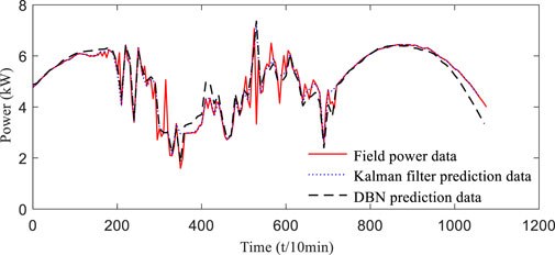
FIGURE 10. Comparison curve of Kalman filter and DBN prediction result.

FIGURE 11

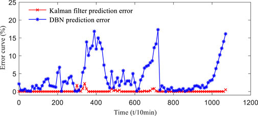
FIGURE 11. Comparison curve of Kalman filter and DBN prediction error.

The simulation experiment is conducted on a personal computer with Intel Core i5-6,400 and 8.00 GB RAM. The Kalman filter model spent 7.8 s in the simulation phase, which is efficient enough for most prediction situations. And the DBN model spent a total of 108 s in the simulation phase, which is less efficient. The training data set of the DBN model during prediction is 8,640 sets of data in 30 days, while the Kalman filter model uses real-time prediction, which requires the amount of data such as future weather forecasting and does not require a large amount of historical data.

Conclusions

In this article, a Kalman filter PV power prediction model based on forecasting experience is proposed. Forecasting experience data are determined using the hourly solar irradiance prediction model, NWP data, and PV conversion model calculations. The dynamic equations of the Kalman filter PV power prediction model are determined by fitting the forecasting experience data of irradiance and PV power. The measured power data are used to dynamically correct the prediction error and limit the residual white noise of the system to realize ultra-short-term prediction of PV power. Finally, using DKASC data and by comparing the analysis with the Kalman filter prediction method based on historical experience and the DBN prediction method, it is verified that the model established in this article has a better prediction accuracy, especially for situations with insufficient historical experience. At the same time, the model in this article has the advantages of low data volume requirement and small computational speed.

Data Availability Statement

The original contributions presented in the study are included in the article/Supplementary Material; further inquiries can be directed to the corresponding author.

Author Contributions

YY has contributed to the conceptualization, writing the original draft, and funding acquisition. TY has contributed to the simulation experiments and writing the original draft. WZ has contributed to giving guidance and providing literature. XZ has contributed to checking the paper for errors and modifying the format of the paper.

Funding

This work was financially supported by the Basic scientific research projects of provincial universities in Heilongjiang Province (2019-KYYWF-0717).

Conflict of Interest

The authors declare that the research was conducted in the absence of any commercial or financial relationships that could be construed as a potential conflict of interest.

Publisher’s Note

All claims expressed in this article are solely those of the authors and do not necessarily represent those of their affiliated organizations, or those of the publisher, the editors, and the reviewers. Any product that may be evaluated in this article, or claim that may be made by its manufacturer, is not guaranteed or endorsed by the publisher.

Supplementary Material

The Supplementary Material for this article can be found online at: https://www.frontiersin.org/articles/10.3389/fenrg.2021.682852/full#supplementary-material

References

Atique, S., Noureen, S., Roy, V., and Bayne, S. (2019). Forecasting of Total Daily Solar Energy Generation Using ARIMA: A Case Study. In 2019 IEEE 9th Annual Computing and Communication Workshop and Conference (CCWC), Las Vegas. University of Nevada. doi:10.1109/ccwc.2019.8666481

CrossRef Full Text | Google Scholar

Bacher, P., Madsen, H., and Nielsen, H. A. (2009). Online Short-Term Solar Power Forecasting. Solar Energy. 83, 1772–1783. doi:10.1016/j.solener.2009.05.016

CrossRef Full Text | Google Scholar

Bingzhong, W. (1999). Sun Position Calculation Relative to the Slope. Solar Energy. 3, 8–9. doi:10.3969/j.issn.1003-0417.1999.03.004

CrossRef Full Text | Google Scholar

Bortolini, M., Gamberi, M., and Graziani, A. (2014). Technical and Economic Design of Photovoltaic and Battery Energy Storage System. Energ. Convers. Management. 86, 81–92. doi:10.1016/j.enconman.2014.04.089

CrossRef Full Text | Google Scholar

Chicco, G., Cocina, V., Di Leo, P., Spertino, F., and Massi Pavan, A. (2016). Error Assessment of Solar Irradiance Forecasts and AC Power from Energy Conversion Model in Grid-Connected Photovoltaic Systems. Energies. 9, 8. doi:10.3390/en9010008

CrossRef Full Text | Google Scholar

De Soto, W., Klein, S. A., and Beckman, W. A. (2006). Improvement and Validation of a Model for Photovoltaic Array Performance. Solar Energy. 80, 78–88. doi:10.1016/j.solener.2005.06.010

CrossRef Full Text | Google Scholar

DKASC (2019). Available at: http://dkasolarcentre.com.au/

Dong, N., Chang, J.-F., Wu, A.-G., and Gao, Z.-K. (2020). A Novel Convolutional Neural Network Framework Based Solar Irradiance Prediction Method. Int. J. Electr. Power Energ. Syst. 114, 105411. doi:10.1016/j.ijepes.2019.105411

CrossRef Full Text | Google Scholar

Galanis, G., Papageorgiou, E., and Liakatas, A. (2017). A Hybrid Bayesian Kalman Filter and Applications to Numerical Wind Speed Modeling. J. Wind Eng. Ind. Aerodynamics. 167, 1–22. doi:10.1016/j.jweia.2017.04.007

CrossRef Full Text | Google Scholar

Hassanzadeh, M., Etezadi, A. M., and Fadali, M. S. (2010). Practical Approach for Sub-Hourly and Hourly Prediction of PV Power Output. North Am. Power Symp. (Naps) 2010, 1–5. doi:10.1109/NAPS.2010.5618944

CrossRef Full Text | Google Scholar

IRENA (2020). Available at: https://www.irena.org/

Khan, I., Zhu, H., Yao, J., Khan, D., and Iqbal, T. (2017). Hybrid Power Forecasting Model for Photovoltaic Plants Based on Neural Network with Air Quality index. Int. J. Photoenergy 2017, 1–9. doi:10.1155/2017/6938713

CrossRef Full Text | Google Scholar

Liu, F., Li, R., Li, Y., Yan, R., and Saha, T. (2017). Takagi-Sugeno Fuzzy Model‐Based Approach Considering Multiple Weather Factors for the Photovoltaic Power Short‐Term Forecasting. IET Renew. Power Generation. 11, 1281–1287. doi:10.1049/iet-rpg.2016.1036

CrossRef Full Text | Google Scholar

Meng, X., Xu, A., Zhao, W., Wang, H., Li, C., and Wang, H. (2018). A New PV Generation Power Prediction Model Based on GA-BP Neural Network with Artificial Classification of History Day. In 2018 International Conference on Power System Technology (POWERCON). China: Guangzhou, 1012–1017. doi:10.1109/POWERCON.2018.8601567

CrossRef Full Text | Google Scholar

NBSLD (1974). Available at: https://www.researchgate.net/publication/234189392 NBSLD computer program for heating and cooling loads in buildings.

Obukhov, S. G., Plotnikov, I. A., and Masolov, V. G. (2018). Mathematical Model of Solar Radiation Based on Climatological Data from NASA SSE. IOP Conf. Series 363, 012021. doi:10.1088/1757-899x/363/1/012021

CrossRef Full Text | Google Scholar

Qing, X., and Niu, Y. (2018). Hourly Day-Ahead Solar Irradiance Prediction Using Weather Forecasts by LSTM. Energy. 148, 461–468. doi:10.1016/j.energy.2018.01.177

CrossRef Full Text | Google Scholar

Qishen, Y. (1986). Building Thermal Processes. Beijing, China: China Construction Industry Press. Available at: https://xueshu.baidu.com/usercenter/paper/show?paperid=3ea1629761f86584006bbffc2f7b7c26&site=xueshu_se.

Salim, A., Agamireddy, T., and Srinivas, K. (2018). Evaluation of Data-Driven Models for Predicting Solar Photovoltaics Power Output. Energy. 142, 1057–1065. doi:10.1016/j.energy.2017.09.042

CrossRef Full Text | Google Scholar

Scolari, E., Sossan, F., and Paolone, M. (2018). Photovoltaic-Model-Based Solar Irradiance Estimators: Performance Comparison and Application to Maximum Power Forecasting. IEEE Trans. Sustain. Energ. 9, 35–44. doi:10.1109/TSTE.2017.2714690

CrossRef Full Text | Google Scholar

Sharadga, H., Hajimirza, S., and Balog, R. S. (2019). Time Series Forecasting of Solar Power Generation for Large-Scale Photovoltaic Plants. Renew. Energ. 150, 797–807. doi:10.1016/j.renene.2019.12.131

CrossRef Full Text | Google Scholar

Singer, S., Rozenshtein, B., and Surazi, S. (1984). Characterization of PV Array Output Using a Small Number of Measured Parameters. Solar Energy. 32, 603–607. doi:10.1016/0038-092X(84)90136-1

CrossRef Full Text | Google Scholar

Wang, K., Qi, X., and Liu, H. (2019). A Comparison of Day-Ahead Photovoltaic Power Forecasting Models Based on Deep Learning Neural Network. Appl. Energ. 251, 113315. doi:10.1016/j.apenergy.2019.113315

CrossRef Full Text | Google Scholar

Xu, W., Mu, C., and Tang, L. (2016). “Advanced Control Techniques for PV Maximum Power point Tracking,” in Advances in Solar Photovoltaic Power Plants (Berlin, Heidelberg: Springer), 43–78. doi:10.1007/978-3-662-50521-2_3

CrossRef Full Text | Google Scholar

Ying, Y., and Tianyang, Y. (2021). Photovoltaic Power Prediction Model Based on NWP Kalman Filter. J. Heilongjiang Univ. Sci. Technology. 31 (01), 92–97. doi:10.3969/j.issn.2095-7262.2021.01.016

CrossRef Full Text | Google Scholar

Zhang, Y., Beaudin, M., Taheri, R., Zareipour, H., and Wood, D. (2015). Day-Ahead Power Output Forecasting for Small-Scale Solar Photovoltaic Electricity Generators. IEEE Trans. Smart Grid. 6, 2253–2262. doi:10.1109/TSG.2015.2397003

CrossRef Full Text | Google Scholar

Zhou, Y., Zhou, N., Gong, L., and Jiang, M. (2020). Prediction of Photovoltaic Power Output Based on Similar Day Analysis, Genetic Algorithm and Extreme Learning Machine. Energy. 204, 117894. doi:10.1016/j.energy.2020.117894

CrossRef Full Text | Google Scholar