 Hao Li
 Ganglin Yu
- Department of Engineering Physics, Tsinghua University, Beijing, China
Decay calculations play an important role in reactor physics simulations. In particular, the isotopic decay of the burned fuel during refueling is important for predicting the startup reactivity of the following burn-up cycle. In addition, there is a growing interest in high-fidelity simulations where the mesh in the burn-up region can involve millions of regions. However, existing models repeatedly solve the same Bateman equations for each region, which is a waste of calculational resources. RMC is a Monte Carlo neutron transport code developed for advanced reactor physics analysis including criticality calculations and burn-up calculations. This paper presents a decay calculation method named the Decay Chain Method (DCM) to optimize the RMC code for large-scale decay calculations. Unlike traditional methods, the Decay Chain Method solves the Bateman equations one decay chain at a time rather than one region at a time. The decay calculation in the burn-up mode then treats the decay steps as zero power burn-up steps with some optimized calculational methods to further reduce the calculational time. These methods were evaluated for a single pin example and for a Virtual Environment for Reactor Applications (VERA) full-core example. The calculations for the single pin example verify the accuracy of the decay step treatment in the burn-up mode and show the improved efficiency. The single pin is divided into 1–1,000,000 decay regions to study the efficiency differences between the Transmutation Trajectory Analysis (TTA) and DCM methods. Both methods have a linear complexity with respect to the number of regions but DCM costs just one-sixtieth of the TTA time. In the simplified VERA full core example, the DCM method reduces the decay calculation time to 0.32 min from 75.26 min while the accuracy remains unchanged.
Introduction
Nuclide concentrations in reactors evolve continuously due to the neutron reactions while running or spontaneous decay during shutdown (Cetnar, 2006). The time evolution of the nuclide concentrations can be described by a set of first-order differential equations, called the Bateman equations (Bateman, 1910). The Bateman equation solutions, which give the burn-up calculations, play an indispensable role in reactor physics simulations.
There is a growing interest in high-fidelity simulations using detailed reactor-core models where the fuel region can be divided into millions of regions. Several full-core benchmarks have been developed, such as the Virtual Environment for Reactor Applications (VERA) (Godfrey, 2014) of the Consortium for Advanced Simulation of Light Water Reactors (CASL) (CASL, 2014; Turinsky and Kothe, 2016), the Nuclear Energy Agency (NEA) Monte Carlo performance benchmark problem (H&M) (Hoogenboom and Martin, 2009) and the MIT PWR (BEAVRS) benchmark (Horelik and Herman, 2012). One common feature of these benchmarks is the huge number of burn-up regions, ranging from thousands to millions of regions. Several Monte Carlo neutron transport codes, such as Serpent2 (Leppänen et al., 2015), MCNP6 (Fensin et al., 2015), MC21 (Griesheimer et al., 2015), VERA-CS (Collins and Godfrey, 2015; Godfrey et al., 2016) and RMC (She et al., 2014; Wang et al., 2015), support burn-up calculation function by coupled to a burn-up calculation module.
The decay calculations are essential because burn-up-decay and burn-up-decay-burn-up problems are common and important in reactor simulations. For example, in the 10th VERA problem, the isotopic decay of the burned fuel is important for predicting the startup reactivity of the following burn-up cycle. The ninth VERA problem includes ten shutdowns, one of which lasted almost 18 days (Godfrey, 2014). However, the computational time for the decay calculations increases with the increasing number of burn-up regions. However, existing models ignore the fact that the same Bateman equations are re-computed a huge number of times with different initial conditions. Thus, a new method is needed to avoid these repetitive calculations and speed up the decay calculations.
This paper introduces the Decay Chain Method (DCM) for decay calculations which is more appropriate for problems with millions of decay regions than traditional methods. This model for decay calculations during burn-up is then incorporated into the RMC code. The decay steps are treated as zero power burn-up steps to simulate burn-up-decay or burn-up-decay-burn-up problems with several methods used to optimize the calculations. Both the accuracy and efficiency of DCM are better than those of existing methods.
Decay Chain Method
Decay and Burnup Equations
We mark a nuclide as i, and mark its atomic density as
In burn-up problems, nuclides are transmuted from one nuclide to another by neutron reactions. Burn-up equations have a similar form to the decay equations with an effective decay constant
The equivalent branching ratio
where
We mark an
The solution to this equation is:
Decay Chain Method
Several neutron transport codes, such as VERA-CS (Collins and Godfrey, 2015), MC21 (Aviles et al., 2017) and RMC (Liu et al., 2017; Wang et al., 2017), have been developed using High Performance Computing (HPC) with parallel processors to handle BEAVRS or VERA fuel-core burn-up calculations where the calculation may involve millions of burn-up regions. RMC solves the burn-up equations with an embedded depletion calculation module named DEPTH (She et al., 2013a). In the traditional method, the burn-up equations are solved one region at a time using the DEPTH module. This method will be called a cell-based method in this paper. In burn-up problems, the matrices differ in different regions. In decay calculations, the elements in the Bateman equation matrix are all constants. Thus, the matrices in all the regions are the same. The cell-based method is applicable to both burn-up and decay problems. However, in decay problems, the same Bateman equations are repeatedly solved in the cell-based method rather than using a more efficient method for very large problems. This paper describes the Decay Chain Method (DCM) that was developed to significantly accelerate the solution of large decay calculations. Unlike the traditional cell-based method, the Decay Chain Method solves the Bateman equations for each mother nuclide to avoid repetitive calculations. The mathematic derivation of the DCM is expressed as follows.
The number of nuclides that need to be taken into consideration is n.
where
Based on Eqs 7, 8, we find that
Comparing Eqs 7, 9, we find that if a concentration vector can be broken up into a linear combination of several different concentration vectors, the concentration vector after decay will still be equal to the linear combination of those concentration vectors.
The following simple example demonstrates the difference between the Decay Chain Method and the traditional cell-based method. For simplicity of writing, the example assumes that there are only three types of nuclides, named N1, N2 and N3, in 4 decay regions, named a, b, c, and d. The initial value of the concentration vector in each region is arbitrarily set and listed in vector form in Table 1. The decay constant of nuclide N1 is ln2 d−1, its daughter nuclide is N2. The decay constant of nuclide N2 is ln
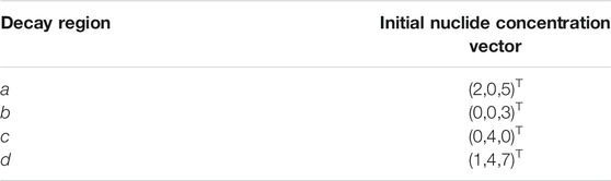
TABLE 1. Initial nuclide concentration vectors in the four decay regions.
In the cell-based methods, the final nuclide concentrations in region a are calculated by the DEPTH module using Eq. 1. Then, the final composition in region b is calculated, with the same method used for regions c and d. The values of the final composition in four regions are also arbitrarily set. The solution process for each region is shown in Figure 1. Thus, the DEPTH module must be called four times.
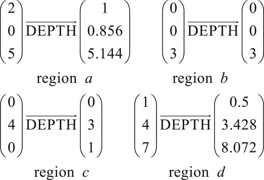
FIGURE 1. Cell-based method solution process for four regions.
The Decay Chain Method uses three unit orthogonal vectors, (1, 0, 0)T, (0, 1, 0)T and (0, 0, 1)T to calculate the final concentrations of the three nuclides in the DEPTH module. Any arbitrary set of three unit orthogonal vectors can be used but this set is most convenient for the calculations. DEPTH provides four algorithms for solving the decay and transmutation equations (She et al., 2013a). They are transmutation trajectory analysis (TTA) (Cetnar, 1999), Chebyshev rational approximation method (CRAM) (Pusa and Leppanen, 2010; Pusa, 2011), Quadrature rational approximation Method (QRAM) and the Laguerre polynomial approximation method (LPAM) (She et al., 2013b). All four solvers in the DEPTH module can be used to calculate the final concentrations with TTA used here due to its efficiency and accuracy (Isotalo and Aarnio, 2011a). The values of the final atomic density of three nuclides are also arbitrarily set. The solution process for every nuclide is shown in Figure 2.
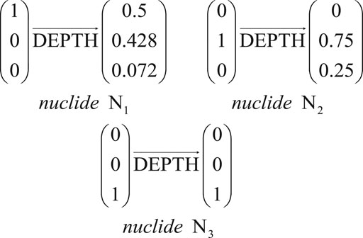
FIGURE 2. Solution process using three unit orthogonal vectors.
Then, the final concentrations in each region are calculated using linear operations of the solution vectors in Figure 2, as shown in Figure 3. The DEPTH module needs to be called just three times in the Decay Chain Method. The vector operations are then very fast compared to the operations needed to solve the decay equations.
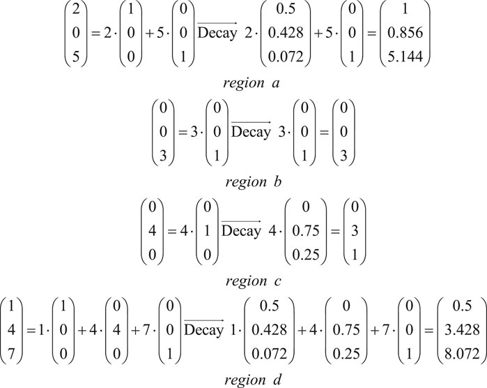
FIGURE 3. Solution process for calculating the nuclide concentrations in four regions.
In problems with 1,500 nuclides and millions of decay regions, the DEPTH module needs to be called only 1,500 times in the Decay Chain Method instead of millions of times in the cell-based method.
The calculation process for the Decay Chain Method is shown in Figure 4.
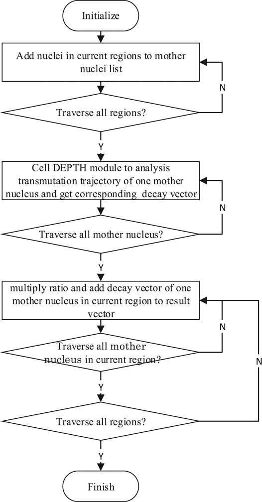
FIGURE 4. Decay Chain Method algorithm.
Decay Calculations in Burnup Mode
The neutron flux drops to almost zero when a reactor is set into shutdown mode from running. The burn-up equations, Eqs 2, 3, can be simplified into the decay equations. Eqs 2, 3 indicate that the decay calculation can be treated as a special case of the burn-up calculation where the power and neutron flux are both zero. Therefore, zero power burn-up steps, which are named decay steps in this paper, are introduced to simulate burn-up-decay and burn-up-decay-burn-up problems.
The decay steps used several optimization methods to improve efficiency and accuracy.
First, the MC neutron transport calculation was bypassed in the decay steps. In normal burn-up calculations, the majority of the computing time is used for the MC calculations to simulate the neutron transport to predict the one-group neutron flux and cross-sections in Eq 2, 3. In the decay steps, the neutron flux is zero, so the product term ϕσj,i becomes zero. Thus, the one-group cross-section is not needed in Eqs 2, 3, so the neutron transport does not need to be simulated.
Second, the burnup strategies like the predictor–corrector method are not needed and the Bateman equations can be simply solved using the starting point approximation method. In burn-up calculations, as shown in Eqs 2, 3, the atomic density of nuclides is determined by the one-group neutron flux and cross-sections. On the other hand, the one-group neutron flux and cross-sections are also influenced by the atomic density of nuclides. To simplify this problem, the starting point approximation method assumes that the one-group neutron flux and cross-sections keep unchanged in one burn-up step. However, this assumption may cause significant error if the one-group neutron flux is large enough. Thus, the predictor-corrector method (Kotlyar and Shwageraus, 2013) use the average of nuclide atomic density at the starting point and the end point to calculate the one-group neutron flux and cross-sections. In burn-up calculations, the predictor-corrector method could get more accurate results than the starting point approximation method. However, in decay calculations, the one-group neutron flux is zero, and the starting point approximation method gives the same results as the predictor–corrector method because the decay matrixes are constants.
Third, the TTA method is used to solve the Bateman equations during the decay steps. TTA outperforms the CRAM method for solving the decay equations (Isotalo and Aarnio, 2011a) although CRAM is more suitable for solving the burn-up equations (Isotalo and Aarnio, 2011a; Pusa, 2011). Since the neutron reactions are not included, the analytical solution of the TTA method provides an efficient solution to the decay equations that is accurate and much faster.
Results and Analysis
Verification of the Decay Steps During the Burnup Mode
The first example used to verify the model is the single pin-cell model taken from the standard Westinghouse 17
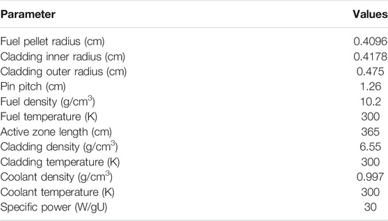
TABLE 2. Physical properties for the first verification example.
The pin was assumed to be depleted to 1,200 MWd/tUs in three burn-up steps, interspersed with a decay step that lasts for 10 days. The RMC used 20,000 particles per cycle with 500 total cycles and 100 inactive cycles for each transport calculation. The Solver, Strategy and Sub-step options were set to the most commonly used values. The Solver option was set to CRAM. The Strategy option was set to predictor-corrector. The Sub-step option was set to 10 (Isotalo and Aarnio, 2011b), which means that each depletion step was divided into 10 sub-steps in the DEPTH module. The ACE data used by RMC was processed from the ENDF/B-VII.0 library.
The calculations with and without the MC transport are referred to as Method 0 and Method 1 in this paper. The calculations without MC transport and using the TTA method is referred to as Method 2. The calculation without MC transport, using the TTA method and adopting the starting point approximation strategy in place of the predictor-corrector strategy during the decay step is referred to as Method 3. The fuel had a total of 644 isotopes after the decay step and atomic densities of the top 50 isotopes at the end of the decay step are presented in Table 3. The atomic density differences of the top 50 nuclides at the end of the decay step predicted by the two methods differed by less than 0.001%. The k-eigenvalues and the wall-clock time are listed in Table 4. The total times for the burnup calculation for the two methods were similar, around 0.022 min.
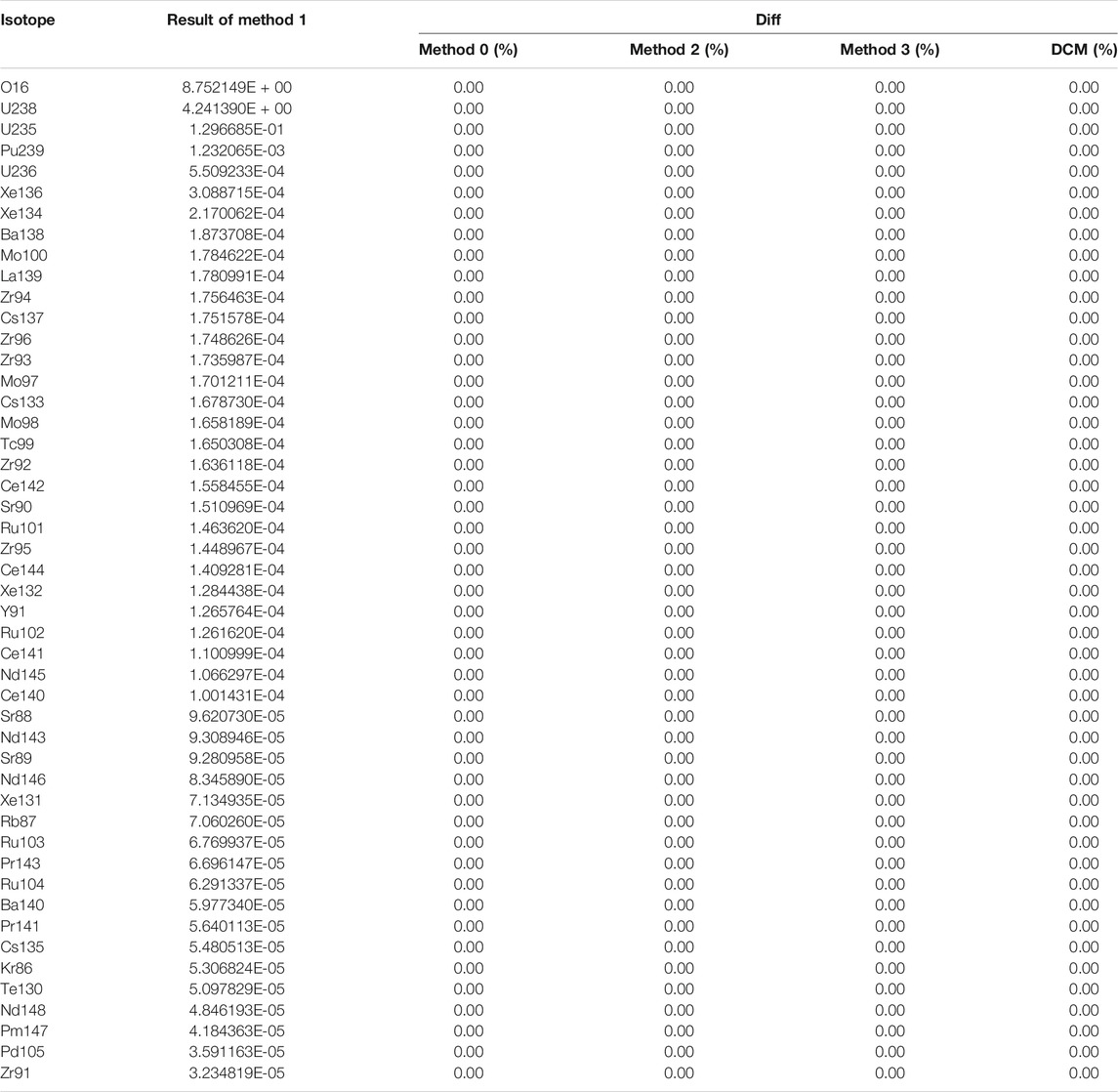
TABLE 3. Atomic densities and differences between different algorithms of top 50 isotopes.
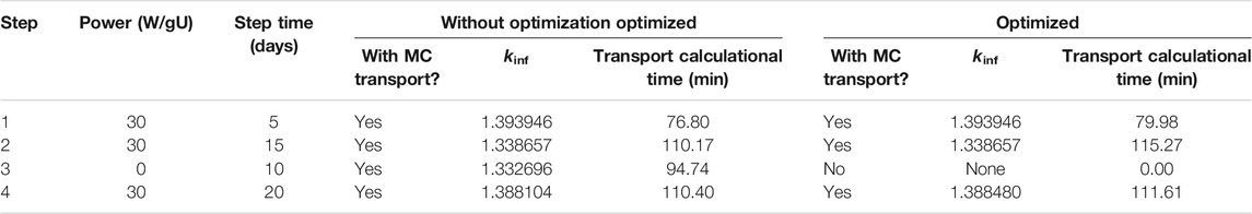
TABLE 4. K-eigenvalues and wall-clock times for the various burnup steps.
The results in Table 4 show that removing the MC transport calculation in the decay step greatly reduces the computational time while keeping the accuracy with the transport calculational time of the third step (the decay step) reduced to zero. The differences in the transport calculational times for the first two steps may be caused by performance fluctuations of the CPUs. In step 1 and 2, the power was not zero and the MC transport must be performed to get the equivalent decay constant and the equivalent branching ratio in Eq. 4, no matter with or without the optimization. Thus, the random number histories in the two methods were the same. In step 3, the power was zero. The optimized method skipped MC transport while the method without optimization did not skip MC transport. From there, the random number histories of the two methods began to differ. Thus, step 1 and 2 in Table 4 exhibit exactly the same kinf values while the k-eigenvalues predicted by the two methods in the fourth step differ by 37.6 pcm with a standard deviation of 18.7 pcm. The difference is no more than two standard deviations, which can be explained by differences in the random number histories.
Accuracy and Efficiency of the Transmutation Trajectory Analysis and Chebyshev Rational Approximation Methods for the Decay Calculation
The accuracies of the TTA and CRAM methods for decay calculations were studied by simulating the decay of Uranium-233. The decay constant of Uranium-233 is 1.3797 × 10⁻¹³ 1/s. The original Uranium-233 density was 1. As shown in Table 5, for normal cases, CRAM and TTA are at the same accuracy level. For decay problems where the neutron flux is zero, TTA is an exact method while CRAM inevitably involves some approximation. In some extreme cases, the error caused by the approximation may be serious. For example, if we extended the decay time to 10 million years, TTA still gave accurate results while the relative error in the CRAM results was more than 77%. We know that a 10 million years’ decay seems a bit impractical, but this extreme case was deliberately designed to verify the robustness of the two methods. The relative error shown in Table 5 indicates that the TTA method is as accurate as the CRAM method in normal cases while the former is more accurate than the latter if the decay time was extremely long. Thus, TTA should be the first choice for decay problems.
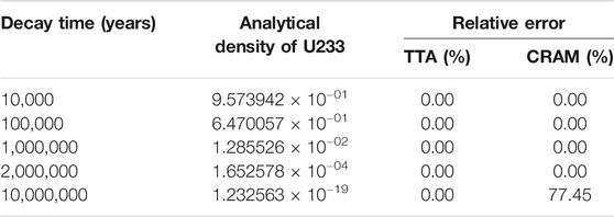
TABLE 5. Uranium-233 density for various decay times and relative errors.
The single pin-cell model was again used to study the influence of the other optimization methods on the efficiency using the same power history, the number of neutrons and cycle conditions as before. The initial nuclide densities were the same as the top 300 nuclide densities at the end of step 2 in the first example. As shown in Table 3, the atomic densities for the top 50 nuclides predicted using Methods 1, 2, 3 and DCM all differed by less than 0.001% with the decay step calculational time listed in Table 6. As we know, the calculational time fluctuates because of the fluctuation of the CPU. To reduce the fluctuation, we re-calculated the single pin-cell problem more than 20 times to get the average calculation time as well as its standard deviation.
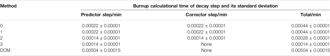
TABLE 6. Decay step calculational times using the various methods.
Efficiencies of Transmutation Trajectory Analysis and Decay Chain Method
The efficiencies of TTA and DCM as the number of decay regions increased were predicted for a single pin divided into 1 to 1,000,000 regions. The initial nuclide densities were the same as the top 300 nuclide densities at the end of step 2 in the first example. We re-calculated problem 5–20 times until the relative standard deviations of the average calculational time reduce to less than 3%. The decay calculational times for the various examples in Figure 5 show that both algorithms have linear complexity. The DCM needs 0.0050 min while TTA needs just 0.0001 min for the one region example since the DEPTH module is called 300 times in DCM but just once in TTA. The DCM calculational times increase to 0.0051 and 0.0052 min for 100 and 1,000 regions. Thus, the calculational time for all the decay chains is around 0.005 min with negligible time for the vector operations in each region. The TTA calculational times exceed those of DCM for more than 100 regions with the gap increasing greatly with the increasing number of regions. The time ratio for the two algorithms stabilizes at around 60 for more than 10,000 regions.
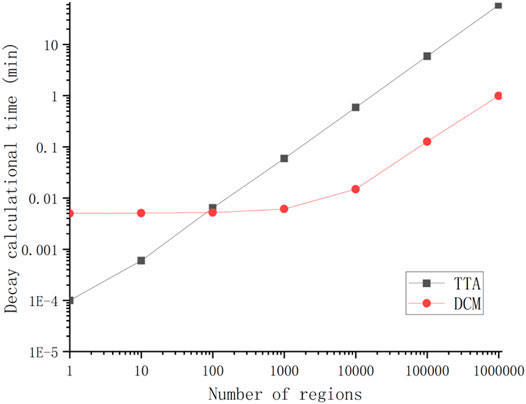
FIGURE 5. Decay calculational times for various numbers of regions.
The DCM calculational times are 0.13 min for 100,000 regions and 0.99 min for 1,000,000 regions. Thus, the calculational time for the vector operations in each region is around 1.0 × 10⁻⁶ min. For 50,000 regions, the calculational time for the vector operations for all the regions is 0.05 min, close to the decay chain calculational time. The vector operations then cost more and more computational time as the number of decay regions increases while decay chain solution time remains unchanged. Thus, the time cost for the DCM calculations gradually changes from constant to linear for more than 10,000 regions. The DCM time is initially constant because the decay chain calculations for all the mother nuclides are independent of the number of regions. The linear increase in the time is then due to the vector operations calculational time being proportional to the number of decay regions.
Decay Part of Virtual Environment for Reactor Applications Problem 10
DCM has been used to simulate the VERA core physics benchmark Problem 10 (Godfrey, 2014). Problem 10 simulates the fuel assembly shuffle involving the refueling outage between two fuel cycles. The isotopic decay of the burned fuel is important when predicting the startup reactivity of the following cycle. Problem 10 simulations using the RMC code are still ongoing (Liang et al., 2016; Liu et al., 2016) but the decay part can be easily simulated using the present model. A simplified example is calculated to study the efficiencies of the different methods. The VERA benchmark problem 10 specifications were taken from Godfrey (2014). The detailed geometry for the full VERA core is shown in Figure 6 which was simulated in RMC. The power history was simplified to three burnup steps as shown in Table 7, i.e., 10 + 10 days of burning and 30 days of wait. Control bank D was withdrawn at 210 steps. Hydraulic and thermal feedback were not taken into consideration. The active core was divided into ten axial segments to give a total of 509,520 burn-up regions. The simulations were run with 100 inactive generations, 500 total generations, and 1,000,000 particles per generation. The calculations were implemented on the TANSUO100 high-performance computer. Each node on TANSUO100 had two Intel Xeon X5670 CPUs with six cores, and each core has 2.10 giga-Hertz of frequency and 12 mega-byte of cache memory. A total of 10 nodes, i.e., 120 cores, were used with 120 MPI parallel processes in each calculation. We re-calculated the problem 5 times to reduce the relative standard deviations of the average calculational time. The calculational times for MC transports range around 370 core
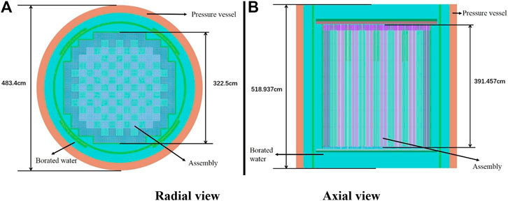
FIGURE 6. The geometry of the full VERA core. (A) Radial view (B) Axial view.
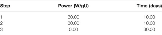
TABLE 7. Power history of simplified VERA problem 10.
The results in Table 8 show that the optimization methods greatly reduce the calculational time for the decay step. The use of the TTA solver rather than the CRAM solver reduced the calculational time for the decay step by almost 40% with the analytical solution of the TTA method giving better accuracy than the CRAM calculation. The removal of the predictor-corrector step nearly halved the calculational time. Finally and most importantly, DCM reduced the calculational time by more than 98%.
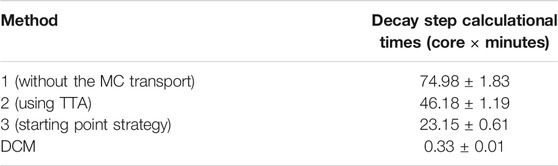
TABLE 8. Decay step calculational times using various methods.
Limitations
The decay chain method can greatly reduce the calculational time for decay steps if the number of fuel regions is very large. However, the decay chain method also has its limitations. First, DCM costs more calculational time than the traditional TTA method if the number of the fuel regions are less than 100. This limitation is acceptable because DCM aims at offering an alternative in some cases rather than completely replace TTA. Users can choose the right method according to the number of fuel regions to play to the strengths of both methods. Second, DCM is only applicable to decay problems where the neutron flux is zero, and is not applicable to burn-up problems where the neutron flux is not zero. The reason is that the neutron flux varies from fuel regions to regions and the transmutation rules vary in different fuel regions even for the same mother nuclide.
Conclusion
Burn-up-decay and burnup-decay-burnup problems are common, important problems in reactor simulations. An efficient decay calculation method, the Decay Chain Method, was developed and validated in this study by optimizing the decay calculations in a burn-up mode calculation in the RMC code.
Unlike traditional methods that solve the Bateman equation cell by cell, the Decay Chain Method first calculates all the decay nuclide chains for each mother nuclide and then calculates the changes in the atomic densities in each cell using solution vector operations. The Decay Chain Method improves the computational efficiency of large decay problems by avoiding repetitively solving the decay equations. In burn-up-decay and burnup-decay-burnup problems, the decay steps are treated as special burn-up steps where the power is 0. Several optimization methods are then used to reduce the computational time cost during the decay steps. The DEPTH module is then only called once for each mother nuclide, which greatly reduces the calculational time. The time complexity of the DCM method changes from constant to linear for more than 10,000 regions. The efficiency is significantly increased with the DCM using only one-sixtieth of the time of traditional methods for more than 10,000 regions. In problems with few regions, the DCM is slightly slower than the traditional methods, but this is still acceptable because small decay problems require very short calculational times. A simplified analysis of VERA Problem 10 involving 509,520 burn-up regions shows that the decay step calculational time is reduced by more than 98%, from 74.98 to 0.33 min with no change in the accuracy.
This work provides a framework for simulating the refueling outage of VERA Problem 10. Future work will consider how to accelerate the full simulation of Problem 10.
Data Availability Statement
The original contributions presented in the study are included in the article/Supplementary Material, further inquiries can be directed to the corresponding author.
Author Contributions
HL: Methodology, Software, Investigation and Writing- Original draft preparation. GY: Methodology, Software, Supervision and Reviewing. SH: Methodology, Supervision, Reviewing and Editing. KW: Methodology and Supervision.
Funding
This work was supported by the Science Challenge Project of China, No. TZ2018001.
Conflict of Interest
The authors declare that the research was conducted in the absence of any commercial or financial relationships that could be construed as a potential conflict of interest.
References
Aviles, B. N., Kelly, D. J., Aumiller, D. L., Gill, D. F., Siebert, B. W., Godfrey, A. T., et al. (2017). MC21/COBRA-IE and VERA-CS Multiphysics Solutions to VERA Core Physics Benchmark Problem #6. Prog. Nucl. Energ. 101, 338–351. doi:10.1016/j.pnucene.2017.05.017
Bateman, H. (1910). The Solution of a System of Differential Equations Occurring in the Theory of Radio-Active Transformations. Proc. Cambridge Philos. Soc. 15, 423–427.
CASL (2014). Consortium for Advanced Simulation of Light Water Reactors (CASL). Available at: http://www.casl.gov
Cetnar, J. (1999). “A Method of Transmutation Trajectories Analysis in Accelerator Driven System,” in Proceedings of the IAEA Technical Committee Meeting on Feasibility and Motivation for Hybrid Concepts for Nuclear Energy Generation and Transmutation, Madrid, 17–19 September 1997.
Cetnar, J. (2006). General Solution of Bateman Equations for Nuclear Transmutations. Ann. Nucl. Energ. 33, 640–645. doi:10.1016/j.anucene.2006.02.004
Collins, B., and Godfrey, A. (2015). “Analysis of the BEAVRS Benchmark Using VERA-CS,” in Joint International Conference on Mathematics and Computation (M&C), Supercomputing in Nuclear Applications (SNA), and the Monte Carlo (MC) Method, Nashville. TN, April 19-23, 2015.
Fensin, M. L., Galloway, J. D., and James, M. R. (2015). Performance Upgrades to the MCNP6 Burnup Capability for Large Scale Depletion Calculations. Prog. Nucl. Energ. 83, 186–190. doi:10.1016/j.pnucene.2015.03.017
Godfrey, A. T., Franceschini, F., Ouisloumen, M., and Kromar, M. (2016). “Simulation of the NPP Krško Cycle 2 with CASL VERA Core Simulator Compared to the CORD2 and PARAGON2/ANC Industrial Code Systems,” in 25th International Conference Nuclear Energy for New Europe (NENE2016), Portoroz, Slovenia, September 5-8, 2016.
Godfrey, A. T. (2014). VERA Core Physics Benchmark Progression Problem Specifications. Revision 4. CASL Technical Report: CASL-U-2012-0131-004.
Griesheimer, D. P., Gill, D. F., Nease, B. R., Sutton, T. M., Stedry, M. H., Dobreff, P. S., et al. (2015). MC21 v.6.0 - A Continuous-Energy Monte Carlo Particle Transport Code with Integrated Reactor Feedback Capabilities. Ann. Nucl. Energ. 82, 29–40. doi:10.1016/j.anucene.2014.08.020
Hoogenboom, J. E., and Martin, W. R. (2009). “A Proposal for a Benchmark to Monitor the Performance of Detailed Monte Carlo Calculation of Power Densities in a Full Size Reactor Core,” in International Conference on Mathematics, Computational Methods & Reactor Physics (M&C 2009), Saratoga Springs, New York, 3-7 May, 2009.
Horelik, N., and Herman, B. (2012). Benchmark for Evaluation and Validation of Reactor Simulations. MIT Computational Reactor Physics Group. URL:<http://crpg.mit.edu/pub/beavrs>
Isotalo, A. E., and Aarnio, P. A. (2011a). Comparison of Depletion Algorithms for Large Systems of Nuclides. Ann. Nucl. Energ. 38, 261–268. doi:10.1016/j.anucene.2010.10.019
Isotalo, A. E., and Aarnio, P. A. (2011b). Substep Methods for Burnup Calculations with Bateman Solutions. Ann. Nucl. Energ. 38, 2509–2514. doi:10.1016/j.anucene.2011.07.012
Kotlyar, D., and Shwageraus, E. (2013). On the Use of Predictor-Corrector Method for Coupled Monte Carlo Burnup Codes. Ann. Nucl. Energ. 58, 228–237. doi:10.1016/j.anucene.2013.03.034
Leppänen, J., Pusa, M., Viitanen, T., Valtavirta, V., and Kaltiaisenaho, T. (2015). The Serpent Monte Carlo Code: Status, Development and Applications in 2013. Ann. Nucl. Energ. 82, 142–150. doi:10.1016/j.anucene.2014.08.024
Liang, J., Wang, K., Qiu, Y., Chai, X., and Qiang, S. (2016). Domain Decomposition Strategy for Pin-wise Full-Core Monte Carlo Depletion Calculation with the Reactor Monte Carlo Code. Nucl. Eng. Technol. 48, 635–641. doi:10.1016/j.net.2016.01.015
Liu, S., Liang, J., Wu, Q., Guo, J., Huang, S., Tang, X., et al. (2017). BEAVRS Full Core Burnup Calculation in Hot Full Power Condition by RMC Code. Ann. Nucl. Energ. 101, 434–446. doi:10.1016/j.anucene.2016.11.033
Liu, S., Yuan, Y., Yu, J., and Wang, K. (2016). Development of On-The-Fly Temperature-dependent Cross-Sections Treatment in RMC Code. Ann. Nucl. Energ. 94, 144–149. doi:10.1016/j.anucene.2016.02.026
Pusa, M., and Leppänen, J. (2010). Computing the Matrix Exponential in Burnup Calculations. Nucl. Sci. Eng. 164, 140–150. doi:10.13182/nse09-14
Pusa, M. (2011). Rational Approximations to the Matrix Exponential in Burnup Calculations. Nucl. Sci. Eng. 169, 155–167. doi:10.13182/nse10-81
She, D., Liang, J., Wang, K., and Forget, B. (2014). 2D Full-Core Monte Carlo Pin-By-Pin Burnup Calculations with the RMC Code. Ann. Nucl. Energ. 64, 201–205. doi:10.1016/j.anucene.2013.10.008
She, D., Liu, Y., Wang, K., Yu, G., Forget, B., Romano, P. K., et al. (2013a). Development of Burnup Methods and Capabilities in Monte Carlo Code RMC. Ann. Nucl. Energ. 51, 289–294. doi:10.1016/j.anucene.2012.07.033
She, D., Zhu, A., and Wang, K. (2013b). Using Generalized Laguerre Polynomials to Compute the Matrix Exponential in Burnup Equations. Nucl. Sci. Eng. 175, 259–265. doi:10.13182/nse12-48
Turinsky, P. J., and Kothe, D. B. (2016). Modeling and Simulation Challenges Pursued by the Consortium for Advanced Simulation of Light Water Reactors (CASL). J. Comput. Phys. 313, 367–376. doi:10.1016/j.jcp.2016.02.043
Wang, K., Li, Z., She, D., Liang, J. g., Xu, Q., Qiu, Y., et al. (2015). RMC - A Monte Carlo Code for Reactor Core Analysis. Ann. Nucl. Energ. 82, 121–129. doi:10.1016/j.anucene.2014.08.048
Keywords: decay chain method, transmutation trajectory analysis, large-scale burnup calculation, virtual environment for reactor applications (VERA), reactor Monte Carlo code (RMC)
Citation: Li H, Yu G, Huang S and Wang K (2021) Optimizing the RMC Code Using the Decay Chain Method for Large-Scale Decay Calculations. Front. Energy Res. 9:676889. doi: 10.3389/fenrg.2021.676889
Received: 06 March 2021; Accepted: 23 June 2021;
Published: 08 July 2021.
Edited by:
Shoaib Usman, Missouri University of Science and Technology, United StatesReviewed by:
Tengfei Zhang, Shanghai Jiao Tong University, ChinaJinfeng Li, Imperial College London, United Kingdom
Copyright © 2021 Li, Yu, Huang and Wang. This is an open-access article distributed under the terms of the Creative Commons Attribution License (CC BY). The use, distribution or reproduction in other forums is permitted, provided the original author(s) and the copyright owner(s) are credited and that the original publication in this journal is cited, in accordance with accepted academic practice. No use, distribution or reproduction is permitted which does not comply with these terms.
*Correspondence: Shanfang Huang, U2ZodWFuZ0BtYWlsLnRzaW5naHVhLmVkdS5jbg==