 Houjun Gong
 Mengqi Wu
95% of researchers rate our articles as excellent or good
Learn more about the work of our research integrity team to safeguard the quality of each article we publish.
Find out more
ORIGINAL RESEARCH article
Front. Energy Res. , 09 June 2021
Sec. Process and Energy Systems Engineering
Volume 9 - 2021 | https://doi.org/10.3389/fenrg.2021.674615
This article is part of the Research Topic Simulation and Modeling of Multiphase Transport in Industrial Process and Facility View all 4 articles
Marine reactors are subjected to additional motions due to ocean conditions. These additional motions will cause large fluctuation of flow rate and change the coolant flow field, making the system unstable. Therefore, in order to understand the effect of oscillating motion on the flow characteristics, a numerical simulation of fluid flow is carried out based on a full-scale three-dimensional oscillating marine reactor. In this study, the resistance coefficients of the lattice, rod buddle and steam generator are fitted, and the distribution of flow rate, velocity as well as pressure in different regions is investigated through the standard model. After additional oscillation is introduced, the flow field in an oscillating reactor is presented and the effect of oscillating angle and elevation on the flow rate is investigated. Results show that the oscillating motion can greatly change the flow field in the reactor; most of the coolant circulates in the downcommer and lower head with only a small amount of coolant entering the core; the flow fluctuation period is consistent with the oscillating period, and the flow variation patterns under different oscillating conditions are basically the same; since the flow amplitude is related to oscillating speed, the amplitude of flow rate rises when decreasing the maximum oscillating angle; the oscillating elevation has little effect on the flow rate.
With high energy density and efficiency, nuclear reactors are widely used, not only for land-based nuclear power plants and research reactors, but also as propulsion power sources for military nuclear power ships, icebreakers, floating platforms and deep-sea probes. However, unlike land-based nuclear reactors, marine reactors normally operate in a dramatically changing marine environment, where they are subjected to additional motions such as heeling, heaving, rolling and pitching generated by ocean waves (Beom et al., 2019). All the ocean motions may have a tendency of making the system more unstable, posing a potential threat to the operational safety of the reactor (Yun et al., 2008). Therefore, when evaluating the reliability and stability of the marine reactor systems, theses additional motions must be taken into account.
Oscillation motion is very common in various offshore platforms and has attracted extensive attention. It not only changes the position of the reactor but also introduces additional three-dimensional acceleration that differ in frequency, direction and amplitude (Yun et al., 2008; Tan et al., 2013). As a consequence, the flow rate and the pressure drop of the coolant system fluctuate, which leads to a significant change in flow field and natural circulation, and may even have deleterious effect on the reactor performance (Iyori et al., 1987; Pendyala et al., 2008; Zhang et al., 2009). Previous studies have shown that these additional motions will affect the flow and heat transfer characteristics of reactor coolant (Ishida et al., 1990; Du and Zhang, 2012; Jie, 2020). Overall, the effect of additional motion can be divided into two aspects: one is to change the natural circulation characteristics of the reactor system, resulting in large fluctuation of flow rate (Hiroyuki et al., 2002; Ishida and Yoritsune, 2002; Gong et al., 2014); the other is to change the coolant flow field in the core to form a coolant stagnation zone and a countercurrent zone in the core (Murata et al., 2012; Gong et al., 2013).
Su et al. (1996) studied the natural circulation flow of the ship reactor’s residual heat removal system under inclination and fluctuation. Gao et al. (1997) established a mathematical model of the primary loop coolant flow affected by marine conditions, and analyzed the influence of the coolant force and various additional inertial accelerations on the coolant flow fluctuation. Kim et al. (2001) reported the natural circulation characteristics of an integral type marine reactor under upright conditions and inclination. It was indicated that the flow rate varies with the angle of the inclination.
Murata et al. (1990, 2002) carried out a series of single-phase natural circulation tests in a model reactor to clarify the effect of rolling motion. The results indicated the loop flow rate in each leg changes periodically with the rolling angle due to the inertial force. Similary, Tan et al. (2009), Huang et al. (2012), Zhu et al. (2019) studied the flow and heat transfer charateristics under rolling motion experimentally. It was found that the flow rate fluctuates periodically due to the additional accelerations.
It is worth noting that under natural circulation or accident conditions, the coolant in the reactor will flow at a low speed. Due to its small inertia, the ability to maintain the original motion is relatively weak, and it is susceptible to additional motions such as tilting, rolling and undulating. Therefore, in the view of marine reactor safety, it is necessary to study the fluid flow in an oscillating reactor. Submarine nuclear reactors should be able to withstand certain lateral and longitudinal oscillation and acceleration movement, and can operate safely and reliably under the marine environment.
Compared with traditional reactors, marine reactors have more severe operation conditions, more compact reactor layout and higher requirements for reactor thermal hydraulic design. At present, pressurized water reactor (PWR) is commonly used in marine reactors. The primary and secondary circuits of the reactor need to be designed in a smaller space, with the reactor pressure vessel (RPV), main pumps, steam generator (SG) and other components all arranged in the containment. In addition, during the operation of a marine reactor, the reactor will fluctuate and oscillates with the hull under the action of wave on the ship. These conditions will affect the flow patterns inside the reactor, which in turn will affect the temperature field distribution in the reactor.
For all these considerations, this paper is aimed to explore the influence of oscillation on the flow field inside an integrated marine reactor by means of CFD simulation which has a great potential to predict the flow characteristics in nuclear reactors as demonstrated in many other works (Du Toit et al., 2006; Boyd, 2016; Wang et al., 2021). For comparison, the flow distribution, velocity profile and pressure distribution under standard condition are also explored. The numerical model is based on a full-scale reactor, including the lower head of pressure vessel, core barrel, lower core plate, fuel assembly, reactor main pump, core shroud, upper core plate, control rod guide tube, steam generator, downcomer and other components. In this paper, the flow characteristics in different regions are analyzed and the fluid flows under different oscillating angle and elevation are also compared.
The flow in the reactor satisfies three conservation equations of fluid, namely mass continuity, momentum conservation and energy conservation.
The mass conservation is expressed as
The equation of energy conservation is
The equation of momentum conservation can be expressed as
where Si is the momentum source term introduced by the porous medium model, which can be denoted as
where 1/α and C2 are viscous resistance coefficient and inertia resistance coefficient, respectively, which need to be determined by fine mesh modeling of local structure.
Besides, when the reactor is subjected to ocean motions which can produce additional accelerations, those accelerations must be introduced into field equations, as discussed in Oscillating Motion.
Shear Stress Transport (SST) turbulence model is one of the
where k and
where the blending fuction F1 is defined by
And the second blending function F2 is described as
The turbulence generation terms
The turbulent dissipation terms
In this study, porous media model is employed to help simulate the pressure drop and the flow resistance inside the reactor. And the areas where the porous media model is adopted mainly include the core fuel assembly area and the steam generator area.
For single-phase and multiphase media, porous media model can take the form of apparent velocity or physical velocity. Assuming that the fluid is single phase, the velocity of the fluid flowing through the area is called the apparent velocity, which can be described as the flow rate through unit cross-sectional area. The porous media model based on apparent velocity can better simulate the pressure loss in porous media. The resistance of fluid in porous materials is calculated by adding a source term to the Navier-Stokes equation, which determines the velocity and pressure field within a fluid domain. The source term mainly consists of inertia loss term and Darcy viscous resistance term, which can be expressed as:
here, Cij and Dij are the coefficient matrices of inertia loss and viscous loss, respectively. The pressure drop in the porous media unit is produced by this negative momentum source term.
For simple homogeneous porous media, the diagonal terms 1/α and C2 are introduced into the coefficient matrix Cij and Dij, respectively, while the other terms are zero, so Si is given as follows:
where 1/α and C2 are viscous resistance coefficient and inertia resistance coefficient, respectively.
When the flow in the porous medium is laminar, the pressure drop is proportional to the velocity, which means the porous medium model can be simplified as Darcy’s Law:
Thus, the pressure drop in the three coordinate directions is given as follows:
where Δni represents the thickness of the porous medium in three coordinate directions.
When the speed is relatively high, or when simulating porous plates and tube rows, the viscous loss term sometimes can be ignored, and only the inertial loss term is retained, hence the porous media equation can be simplified to:
or given as the pressure drop in three coordinate directions:
In a porous medium, when the permeability of the medium is large and the geometric scale of the medium does not interact with the scale of the turbulent vortex, it can be considered that the solid matrix has no effect on the generation and dissipation rate of turbulence.
With regard to resistance coefficient, it is generally defined based on the apparent velocity of fluid in porous media. In this study, the inertia resistance coefficient and viscous resistance coefficient are determined by the relationship between pressure drop Δp and velocity v in porous media. Suppose the second-order polynomial fitting relationship between pressure drop and velocity is:
where a1 and a2 are fitting coefficients. The source term in the N-S equation is the pressure drop per unit length, which is given as follows:
Then, the resistance coefficients can be obtained bycalculation, which are expressed as follows:
In this simulation, the hybrid mesh method is adopted to mesh the established geometric model. As shown in Figures 1A,B, the area of the lower head and the upper chamber is divided by poly-hexa meshes. By contrast, full hexahedral meshes are used in the inlet section, the descending section of the downcommer, the core and the steam generator area, as shown in Figures 1C,D.
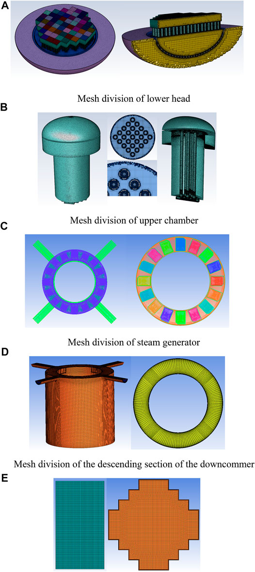
FIGURE 1. Mesh division of different regions. (A) Mesh division of lower head. (B) Mesh division of upper chamber. (C) Mesh division of steam generator. (D) Mesh division of the descending section of the downcommer.
Then, the mesh sensitivity is demonstrated by generating meshes of different scales. Under the same cold state condition, the comparison of pressure drop throughout the reactor with different mesh scales is obtained and the desirable mesh scheme for subsequent calculation can be determined.
Table 1 shows the number of meshes based on different meshing schemes. ICEM is employed to establish hexahedral grid for annulus, core and steam generator area, while Fluent Meshing is used for upper and lower head regions for the Poly-hexa Meshing. In order to get a reasonable computing mesh model, different number of meshes is generated in different regions. Then the whole model is verified under standard conditions to determine the computational mesh model needed for subsequent simulation.
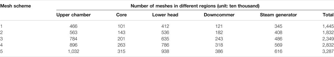
TABLE 1. Description of different mesh schemes.
Figure 2 compares the pressure drop in different regions of the reactor under different mesh schemes. It can be obtained that the average pressure of each area tends to be stable with the increase of grid number. The results of mesh scheme 3, 4, and 5 show little difference, so mesh scheme 3 is employed in subsequent calculation and analysis.
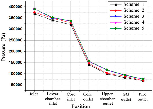
FIGURE 2. Pressure drop in different regions of reactor under different mesh schemes.
As discussed before, the flow in the reactor satisfies three conservation equations of fluid, including mass continuity, momentum conservation and energy conservation. When the reactor system is subjected to additional motions, additional forces or accelerations are generated and must be taken into consideration in governing equations.
In this study, considering the effect of oscillating motion, a volume force is introduced into the momentum equation, which is expressed as:
where
where
The oscillating angle in the oscillating motion can be derived as (Gao, 1999):
where
And the angular velocity and accerelation can be derived as:
By decomposing the additional acceleration, the expression of the additional motion inertia force is obtained as follows:
Three dimensional simulation on the cold state flow field is conducted based on a full-scale marine reactor, considering the influence of gravity and oscillating inertia force. And the transient hydrodynamic analysis of the whole model is carried out. The temperature of water used as coolant is set at 230°C. The energy exchange between the core and steam generator is neglected.
In this research, porous media model is adopted in the core fuel assembly area and the steam generator area. In order to simulate the flow field, the resistance coefficient need to be determined according to the relationship between pressure drop and velocity.
The flow distribution plate and the lower head will directly affect the flow distribution into the core and further influence the local flow field, so it is necessary to perform refined solid modeling with the structure details considered. Through the standard model, the distribution of flow rate, velocity as well as pressure is investigated. Then, after introducing additional oscillation, the effect of oscillating angle and elevation on the flow field is studied.
The oscillating models are listed in Table 2 with different oscillating angles and elevations. The completed calculation conditions are consistent with the technical requirements. After the calculation, the flow field and pressure of the core, the lower head, the downcomer and the primary side of the steam generator are presented in the form of streamline and velocity contour. The aim is to explore the influence of oscillating angle and oscillating elevation on the cold hydrodynamics.
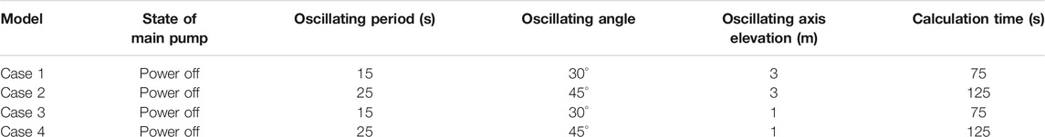
TABLE 2. The oscillating models.
The resistance coefficient can be determined by the relationship between pressure drop and velocity in porous media as described previously in Porous Media Model. In the research, the pressure loss of fuel assembly with lattice is calculated without considering the effect of gravity. According to the pressure at the different selected cross-sections, the pressure loss and the flow resistance of the light rod and the lattice area can be obtained.
As shown in Figure 3, the Z1/Z2 cross-section is extracted to calculate the regional resistance coefficient of the lattice, and the pressure difference of Z3/Z4 cross-section is used to calculate the regional resistance coefficient of the light rod.
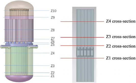
FIGURE 3. The selection of cross sections.
The flow parameters in the rod bundle area are given in Table 3, the pressure loss could be acquired through analyzing the pressure of the upper and lower cross-sections of the light rod. Here, the equivalent velocity refers to the actual velocity in the porous medium model. Compared with the real model, the actual velocity in the porous medium is the actual velocity of the real model multiplied by the porosity.
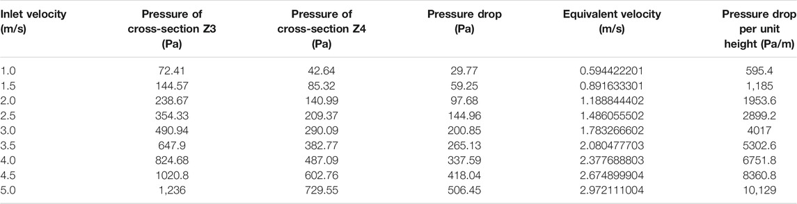
TABLE 3. Flow parameters in the rod bundle area.
And the change of pressure loss per unit height with velocity in the rod bundle area is shown in Figure 4. The relationship between pressure loss per unit length and the velocity can be expressed as follows:
According to Eq. 26, the inertial resistance coefficient
where

FIGURE 4. Relationship between axial resistance and velocity in light rod area.
By analyzing the pressure of the front and rear cross-sections of the light rod area, the pressure loss could be acquired to show the variation of pressure loss per unit length with velocity in the rod bundle area, as presented in Figure 5. And the relationship between pressure loss per unit length and the velocity can be described as:
Through calculation, the inertial resistance coefficient
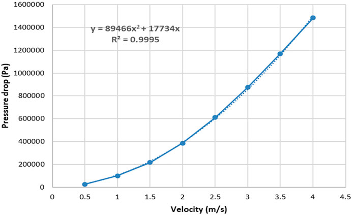
FIGURE 5. Relationship between lateral resistance and velocity in light rod area.
Table 4 shows flow parameters in the lattice area. The pressure of the upper and lower cross-sections of the lattice and the equivalent velocity are presented.
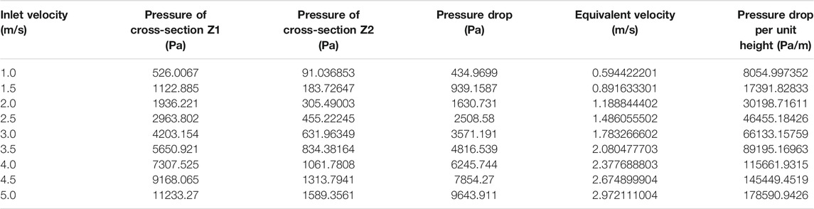
TABLE 4. Flow parameters in the lattice area.
By analyzing the pressure of the upper and lower cross-sections of the grid, the pressure loss could be acquired to show the variation of pressure loss with velocity in the grid area per unit height. Then, the relationship between pressure loss per unit length and the velocity is obtained by fitting velocity-pressure loss per unit height, and the expression can be derived as follows:
According to Eq. 32, the inertial resistance coefficient
Porous medium model is adopted to simulate the flow in the steam generator. Firstly, it’s assumed that overall resistance coefficient along the 1-D flow direction is uniform. According to the experimentally measured pressure loss of SG under specific flow rate, the relationship between pressure loss per unit length and the velocity can be expressed as follows:
Both the reactors with and without additional movements are studied. For the standard model, no additional motion is imposed to the reactor in order to show the original flow field. The boundary conditions for the two types of model are explained in the following.
The boundary conditions for standard models are as follows:
1) Inlet boundary: the inlet flow rate is constant and set at 2,289 kg/s;
2) Outlet boundary conditions: the outlet pressure is fixed, the gauge pressure is 0Pa, the reference pressure is 15.0 Mpa;
3) Core: the porosity is 0.594, the porous media model is adopted, and the axial and lateral resistance coefficients are given;
4) Steam generator: the porosity is 0.55, the porous media model is adopted, and the axial and lateral resistance coefficients are given;
5) The interface is used to for mesh connection between each area.
The boundary conditions for oscillating models are as follows:
1) No inlet/outlet boundary conditions;
2) Core: the porosity is 0.594, porous media model is adopted, and the axial and lateral resistance coefficients are given;
3) Steam generator: the porosity is 0.55, porous media model is adopted, and the axial and lateral resistance coefficients are given;
4) The interface is used to for mesh connection between each area;
5) Oscillating motion: the momentum source terms related to oscillation are added to each region of the reactor, respectively. The momentum source term is in the form of UDF (User-Defined Function). The oscillating axis in this calculation is x-axis. Therefore, the momentum source terms to be added are momentum source terms in Y and Z directions. The expression can be seen in Oscillating Motion;
6) Gravity equation: the relationship between gravity direction and time should be considered in this calculation. Based on fluent expression, gravity is projected in Y/Z direction to realize real-time adjustment of gravity with oscillating motion.
For comparison, the flow field in a static reactor is studied first in Standard Model. No additional motion is imposed to the reactor. The inlet flow distribution, velocity field, and pressure are discussed in this part.
Through the simulation of standard working condition, the distribution of flow rate at core inlet is obtained and presented in Figure 6A. The highest normalized mass flow at the core inlet is 1.034 and the lowest normalized flow is 0.979, indicating that the reactor core inlet flow distribution is fairly uniform with the maximum positive and negative deviation within 6%.
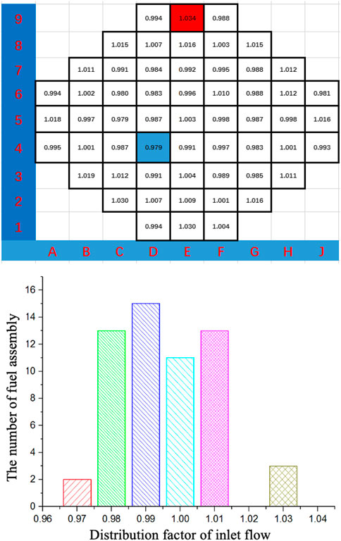
FIGURE 6. Flow distribution at core inlet. (A) Normalized flow distribution at core inlet. (B) The number of fuel assemblies with different inlet flow distribution factors.
Figure 6B shows the number of fuel assemblies arranged in areas with different inlet flow distribution factor. The horizontal coordinate is the flow distribution factor at core inlet, which is mainly distributed between 98 and 102%. And there are 52 groups of fuel assemblies in these regions. In addition, the distribution of inlet flow is generally uniform, with only five fuel assemblies arranged in the area where the deviation of flow distribution factor is greater than 2%.
Figure 7A shows the velocity vector and velocity contour of Z4 cross-section in downcommer. It can be obtained that there is an evident transverse flow in the downcommer section at the inlet of the downcommer section due to the effect of the inlet. Figure 7B shows the velocity vector and velocity contour in the lower head area of cross-section sec45. Results show that in the lower head area, the velocity in the flow distribution pipe around the central area is higher than that in the upper side area. And the flow velocity near the lower tube seat is relatively uniform.
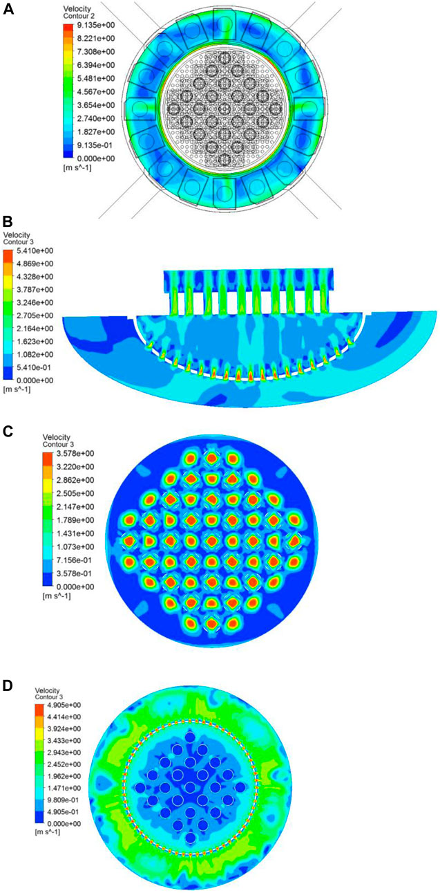
FIGURE 7. Velocity distribution in different regions. (A) Velocity distribution of Z4 cross-section in downcommer. (B) Velocity distribution of Sec45 cross-section in lower head. (C) Velocity distribution of Z7 cross-section in upper chamber. (D) Velocity distribution of Z10 cross-section in upper chamber.
Figures 7C,D present the velocity distribution in the upper chamber area of cross-section Z7 and Z10, respectively. It can be seen from Figure 7C that in the lower region of the guide tube, the fluid enters the upper chamber through the upper plate of the core, and mainly moves in the axial direction, and the transverse flow occurs at the opening of the guide tube. By contrast, the fluid near the Z10 cross-section in the upper chamber flows to the steam generator through the top opening, and the flow velocity is higher at the opening position.
Table 5 shows the pressure at different positions of the reactor and compares the pressure loss in each area. The pressure loss from the inlet to the outlet is about 0.314 MPa under standard conditions, and the pressure loss in the core area is about 0.05 Mpa. It is worth noting that gravity loss is concluded in the pressure loss.
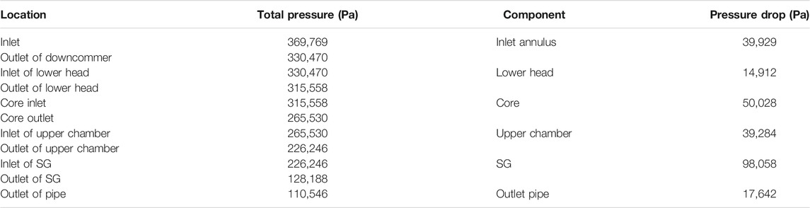
TABLE 5. Pressure loss in each region of reactor.
The pressure distribution in the reactor is presented in Figure 8, which indicates that the maximum total pressure in the reactor from the inlet to outlet is about 0.39 MPa. Along the flow direction, the total pressure in the reactor gradually decreases.
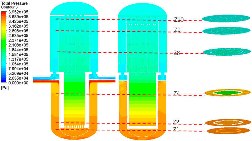
FIGURE 8. Pressure contour in the reactor.
This part focuses on the flow characteristics under oscillating motion. The influene of the oscillating motion is presented by comparing the fluid flow under four different oscillation models, which are introduced in Simulation Model and Conditions. The results of flow field distribution, different oscillating angles and different elevations are analyzed as follows.
When the reactor is subjected to oscillating motion, the flow characteristics will be greatly changed. Here, the flow field in an oscillating reactor with an oscillating angle of 45° and an oscillating period of 25 s is presented. Figure 9 compares the velocity vector in different regions.
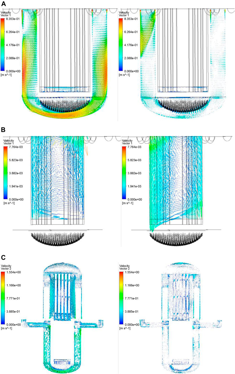
FIGURE 9. The comparison of velocity vector in an oscillating reactor. (A) The velocity of cross‐section X = 0 m of the downcommer and lower head at the time of max oscillating angle. (B) The velocity of cross‐section X = 0 m of the core at the time of max oscillating angle. (C) The velocity of cross‐section X = 0 m of the reactor loop.
Figure 9A shows the velocity vector of the cross-section X = 0 m of the downcommer and lower head at different moments. In an oscillating reactor, most of the coolant forms a circulating flow in the downcommer and the outer region of the distribution plate in the lower head. By contrast, only a small amount of coolant can enter the core through the rectification hole.
With regard to the flow field in the core, it can be seen form Figure 9B that during the oscillation motion, the coolant in the core region forms two obvious vortex flows, which are, respectively located in the upper part and the lower part of the core.
The velocity distribution in the reactor loop is shown in Figure 9C. It is noticed that the flow inside the upper and lower heads is more obvious than that inside the core. The flow direction is consistent with the oscillating direction of the reactor.
Figure 10A shows the streamline distribution in the reactor under oscillating motion. Due to the effect of oscillation, there are obvious vortex flows inside the descending annulus and the upper chamber, and the fluid forms its own circulating flow in these regions. On the contrary, the flow in the core and steam generator area is not apparent.
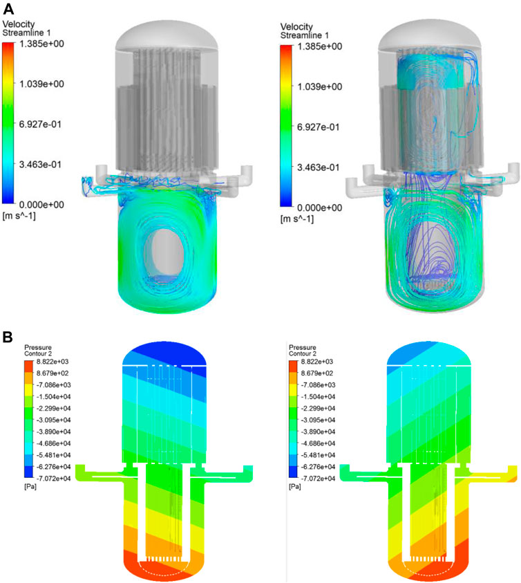
FIGURE 10. The overall flow and pressure distribution. (A) Streamline distribution in an oscillating reactor. (B) Pressure distribution in an oscillating reactor.
Figure 10B presents the pressure distribution of the reactor loop at different times. It can be obtained that the pressure in the reactor changes as the reactor oscillates. This is because the relative position changes during the oscillating process. Consequently, the pressure in an oscillating reactor presents an inclined distribution.
To compare the influence of oscillating angle on the fluid flow, we explore the flow rate in the steam generators because they are intimately associated with a stable reactor operation. From the perspective of reactor safety, the automatic control system for the water level should be able to operate smoothly without any oscillation or hunching; however, in the marine environment, the acceleration and oscillation motion of the ship can easily affect the water level of SGs (Ishida et al., 1995).
The arrangement of SGs in the reactor can be seen in Figure 7A. Due to the symmetrical arrangement of the steam generators, subsequent analysis only focus on SG1-SG5. The oscillating axis is along the line between SG1 and SG9.
Figure 11 compares the flow rate in different steam generators under two oscillating angles (the oscillating elevation is 3 m). It can be found that the flow fluctuation period is consistent with the oscillating period, and the flow variation patterns under different oscillating angles are basically the same. For SG1 which is located on the oscillating axis, two peaks can be noticed in one cycle although the second peak is significantly smaller than the first. By contrast, the change of flow rate in other steam generators shows a cosine distribution.
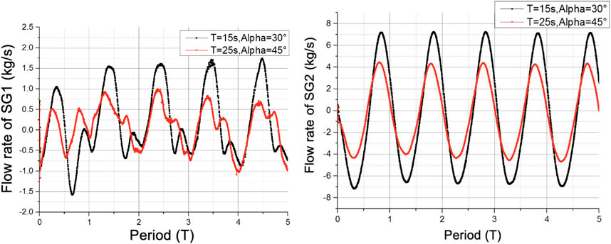
FIGURE 11. The change of flow rate under different oscillating angles.
Besides, the SG flow rate under the oscillating angle of 30° is greater than that under the angle of 45°. This is because the relative rotation speed of the 30° working condition is higher than that of the 45° working condition, which makes the flow velocity in the SG during the oscillating process much higher. As a consequence, the mass flow amplitude rises when decreasing the maximum oscillating angle.
It can also be obtained that the amplitude of flow rate is related to oscillating speed. Due to the displacement of oscillating axis between SG1 and SG9, the mass flow amplitude of SG1-SG5 gradually increases. The amplitudes of flow rate in SG1-SG5 is shown in Figure 12. The horizontal coordinate represents the angle between the steam generator and the oscillating axis. SG5 is the farthest from the oscillating center with the maximum linear velocity, therefore its amplitude of the flow rate is the largest.
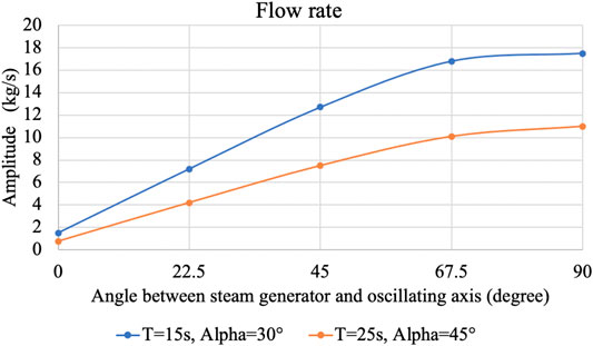
FIGURE 12. The amplitude of flow rate in SG1-SG5.
Figure 13 shows the comparison of flow rate under two different oscillating elevations (the oscillating angle is 30° and the period is 15 s). Results show that the oscillating elevation has little effect on the flow rate. The change patterns of flow rate in all steam generators under different elevations are basically consistent. The difference of flow amplitude is within 3 kg/s.
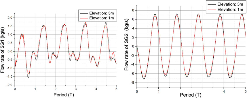
FIGURE 13. Comparison of flow rate under two different oscillating elevations (the oscillating angle is 30° and the period is 15 s).
This paper explores the effect of oscillating motion on the fluid flow in a full-scale reactor through numerical simulation. Shear Stress Transport (SST) turbulence model and Porous media model are adopted. In this study, the resistance coefficients of the lattice, rod buddle and steam generator are fitted according to the relationship between velocity and pressure loss.
Through the simulation of the standard model, the inlet flow distribution, the flow field and the pressure distribution in the reactor are presented. Results show that the distribution of core inlet flow is uniform overall. Transverse flows can be noticed in the downcommer and the opening of the guide tube in the upper chamber, and the total pressure in the reactor gradually decreases along the flow direction.
After additional oscillation is introduced, the flow field inside an oscillating reactor is presented and the influence of oscillating angle and elevation on the flow rate is studied. It is found that the oscillating motion can greatly change the flow characteristics: most of the coolant forms a circulating flow in the downcommer and lower head with only a small amount of coolant entering the core through the rectification hole of the lower head; during the oscillating motion, the coolant in the core region forms two obvious vortex flows; vortex flows can also be observed inside the descending annulus and the upper chamber where the fluid forms its own circulating flow in these area.
In addition, comparisons have been made on the flow rate under different oscillating angle and elevation. It can be concluded that the flow fluctuation period is consistent with the oscillating period, and the flow variation pattern under different oscillating conditions is basically consistent. The flow amplitude is related to oscillating speed, therefore the amplitude of mass flow of SG1-SG5 gradually increases, and it also rises when decreasing the maximum oscillating angle. Besides, the oscillating elevation has little effect on the flow rate.
The original contributions presented in the study are included in the article/Supplementary Material, further inquiries can be directed to the corresponding author.
HG is responsible for meshing of reactor and flow resistance; MW is responsible for cfd simulation.
The authors declare that the research was conducted in the absence of any commercial or financial relationships that could be construed as a potential conflict of interest.
The authors are grateful for the support of this research by the National Science and Technology Major Project (Grant No. 2011ZX06901-003), and the fund of Nuclear Power Technology Innovation Center (Grant Nos. HDLCXZX-2020-HD-022 and HDLCXZX-2021-ZH-024).
Beom, H.-K., Kim, G.-W., Park, G.-C., and Cho, H. K. (2019). Verification and Improvement of Dynamic Motion Model in MARS for marine Reactor thermal-hydraulic Analysis under Ocean Condition. Nucl. Eng. Technol. 51, 1231–1240. doi:10.1016/j.net.2019.02.018
Boyd, C. (2016). Perspectives on CFD Analysis in Nuclear Reactor Regulation. Nucl. Eng. Des. 299, 12–17. doi:10.1016/j.nucengdes.2015.08.001
Du, S. J., and Zhang, H. (2012). Heat Transfer Characteristics of Forced Circulation under Inclined Conditions. Nucl. Power Eng. 3, 46–50. doi:10.3969/j.issn.0258-0926.2012.03.010
Du Toit, C. G, Rousseau, P. G., Greyvenstein, G. P., and Landman, W. A. (2006). A Systems CFD Model of a Packed Bed High Temperature Gas-Cooled Nuclear Reactor. Int. J. Therm. Sci. 45 (1), 70–85. doi:10.1016/j.ijthermalsci.2005.04.010
Gao, P. Z. (1999). Effect of Ocean Conditions upon thermal-hydraulic Properties of Nuclear Power Plant. Ph. D. Thesis. Harbin:Harbin Engineering University.
Gao, P. Z., Pang, F. G., and Wang, Z. X. (1997). Mathematical Model of Primary Coolant in Nuclear Power Plant Influenced by Ocean Conditions. J. Harbin Eng. Univ. 18 (1), 24–27.
Gong, H. J., Yang, X. T., and Huang, Y. P. (2014). Experimental and Numerical Study on Natural Circulation of Integrated Reactor under Inclination Condition. Nucl. Power Eng. 35 (5), 89–93. doi:10.13832/j.jnpe.2014.05.0089
Gong, H. J., Yang, X. T., Huang, Y. P., and Jiang, S. Y. (2013). Study on Flow Characteristics of Integral Reactor Test Facility under Rolling Motion without Heating. Nucl. Power Eng. 3, 77–81. doi:10.3969/j.issn.0258-0926.2013.03.017
Hiroyuki, M., Kenichi, S., and Michiyuki, J. (2002). Natural Circulation Characteristics of a marine Reactor in Rolling Motion and Heat Transfer in the Core. Nucl. Eng. Des. 215 (1-2), 69–85. doi:10.1016/s0029-5493(02)00042-0
Huang, J., Lee, Y., and Park, G. (2012). Characteristics of Critical Heat Flux under Rolling Condition for Flow Boiling in Vertical Tube. Nucl. Eng. Des. 252, 153–162. doi:10.1016/j.nucengdes.2012.06.032
Ishida, I., Kusunoki, T., Murata, H., Yokomura, T., Kobayashi, M., and Nariai, H. (1990). Thermal-hydraulic Behavior of a marine Reactor during Oscillations. Nucl. Eng. Des. 120, 213–225. doi:10.1016/0029-5493(90)90374-7
Ishida, T., Kusunoki, T., Ochiai, M., Yao, T., and Inoue, K. (1995). Effects by Sea Wave on thermal Hydraulics of marine Reactor System. J. Nucl. Sci. Technol. 32 (8), 740–751. doi:10.1080/18811248.1995.9731769
Ishida, T., and Yoritsune, T. (2002). Effects of Ship Motions on Natural Circulation of Deep Sea Research Reactor DRX. Nucl. Eng. Des. 215, 51–67. doi:10.1016/s0029-5493(02)00041-9
Iyori, I., Aya, I., Murata, H., Kobayashi, M., and Nariai, H. (1987). Natural Circulation of Integrated-type marine Reactor at Inclined Attitude. Nucl. Eng. Des. 99, 423–430. doi:10.1016/0029-5493(87)90138-5
Jie, X. (2020). Research Progress of Reactor thermal-hydraulic Characteristics under Ocean Conditions in China. Front. Energ. Res. 8, 593362. doi:10.3389/fenrg.2020.593362
Kim, J.-H., Kim, T.-W., Lee, S.-M., and Park, G.-C. (2001). Study on the Natural Circulation Characteristics of the Integral Type Reactor for Vertical and Inclined Conditions. Nucl. Eng. Des. 207, 21–31. doi:10.1016/s0029-5493(00)00417-9
Menter, F. R., and Esch, T. (2001). “Elements of Industrial Heat Transfer Prediction,” in Proceedings of the 16th Brazilian Congress of Mechanical Engineering (COBEM), Minas Gerais, Brazil, November 26–30, 2001, Uberlandia, Brazil, 26–30.
Menter, F. R., Kuntz, M., and Langtry, R. (2003). “Ten Years of Industrial Experience with the SST Turbulence Model,” in Editors Hanjalic, K., Nagano, Y., and Tummers, M. Proceedings of the 4th International Symposium on Turbulence, Heat and Mass Transfer, October 12-17, 2003, New York, USA, (West Redding: Begell House Inc.). 4, 625–632.
Menter, F. R. (1994). Two-equation Eddy-Viscosity Turbulence Models for Engineering Applications. AIAA J. 32 (8), 1598–1605. doi:10.2514/3.12149
Mohammadi, B., and Pironneau, O. (1993). Analysis of the K-Epsilon Turbulence Model. Paris, France: Wiley.
Murata, H., Iyori, I., and Kobayashi, M. (1990). Natural Circulation Characteristics of a marine Reactor in Rolling Motion. Nucl. Eng. Des. 118, 141–154. doi:10.1016/0029-5493(90)90053-z
Murata, H., Oka, H., Adachi, M., and Harumi, K. (2012). Effects of the Ship Motion on Gas-Solid Flow and Heat Transfer in a Circulating Fluidized Bed. Powder Technol. 231, 7–17. doi:10.1016/j.powtec.2012.06.060
Murata, H., Sawada, K.-i., and Kobayashi, M. (2002). Natural Circulation Characteristics of a marine Reactor in Rolling Motion and Heat Transfer in the Core. Nucl. Eng. Des. 215, 69–85. doi:10.1016/s0029-5493(02)00042-0
Pendyala, R., Jayanti, S., and Balakrishnan, A. R. (2008). Flow and Pressure Drop Fluctuations in a Vertical Tube Subject to Low Frequency Oscillations. Nucl. Eng. Des. 238, 178–187. doi:10.1016/j.nucengdes.2007.06.010
Su, G. H., Zhang, J. L., Guo, Y. J., Qiu, S. Z., Yu, Z. W., and Jia, D. N. (1996). Effects of Ocean Conditions upon the Passive Residual Heat Removal System (PRHRS) of Ship Reactor. At. Energ. Sci. Technol. 30 (6), 487–491.
Tan, S.-C., Su, G. H., and Gao, P.-Z. (2009). Experimental and Theoretical Study on Single-phase Natural Circulation Flow and Heat Transfer under Rolling Motion Condition. Appl. Therm. Eng. 29, 3160–3168. doi:10.1016/j.applthermaleng.2009.04.019
Tan, S., Wang, Z., Wang, C., and Lan, S. (2013). Flow Fluctuations and Flow Friction Characteristics of Vertical Narrow Rectangular Channel under Rolling Motion Conditions. Exp. Therm. Fluid Sci. 50, 69–78. doi:10.1016/j.expthermflusci.2013.05.006
Wang, M., Wang, Y., Tian, W., Qiu, S., and Su, G. H. (2021). Recent Progress of CFD Applications in PWR thermal Hydraulics Study and Future Directions. Ann. Nucl. Energ. 150, 107836. doi:10.1016/j.anucene.2020.107836
Wilcox, D. C. (1988). Reassessment of the Scale-Determining Equation for Advanced Turbulence Models. AIAA J. 26, 1299–1310. doi:10.2514/3.10041
Yun, G., Qiu, S. Z., Su, G. H., and Jia, D. N. (2008). The Influence of Ocean Conditions on Two-phase Flow Instability in a Parallel Multi-Channel System. Ann. Nucl. Energ. 35 (9), 1598–1605. doi:10.1016/j.anucene.2008.03.003
Zhang, J.-H., Yan, C.-Q., and Gao, P.-Z. (2009). Characteristics of Pressure Drop and Correlation of Friction Factors for Single-phase Flow in Rolling Horizontal Pipe. J. Hydrodyn. 21 (5), 614–621. doi:10.1016/s1001-6058(08)60192-4
Keywords: oscillating reactor, resistance coefficient, flow field, oscillating angle, oscillating elevation
Citation: Gong H and Wu M (2021) Numerical Simulation of Full-Scale Three-Dimensional Fluid Flow in an Oscillating Reactor. Front. Energy Res. 9:674615. doi: 10.3389/fenrg.2021.674615
Received: 01 March 2021; Accepted: 03 May 2021;
Published: 09 June 2021.
Edited by:
Huang Zhang, Washington University in St. Louis, United StatesReviewed by:
Mingjun Wang, Xi’an Jiaotong University, ChinaCopyright © 2021 Gong and Wu. This is an open-access article distributed under the terms of the Creative Commons Attribution License (CC BY). The use, distribution or reproduction in other forums is permitted, provided the original author(s) and the copyright owner(s) are credited and that the original publication in this journal is cited, in accordance with accepted academic practice. No use, distribution or reproduction is permitted which does not comply with these terms.
*Correspondence: Houjun Gong, Z2hqdHNpbmdAMTI2LmNvbQ==
Disclaimer: All claims expressed in this article are solely those of the authors and do not necessarily represent those of their affiliated organizations, or those of the publisher, the editors and the reviewers. Any product that may be evaluated in this article or claim that may be made by its manufacturer is not guaranteed or endorsed by the publisher.
Research integrity at Frontiers
Learn more about the work of our research integrity team to safeguard the quality of each article we publish.