Advancing the Thermal Network Representation for the Optimal Design of Distributed Multi-Energy Systems

This paper investigates modeling methods with thermal network representation under the scope of the optimal design and operation of Distributed Multi-Energy System (D-MES). Two modeling approaches are compared: A Mixed‐Integer Linear Programming (MILP) optimization model and a district heating network (DHN) simulation model. The MILP model was developed for the simultaneous design of the network layout, the sizing, and locations of energy generation and storage technologies to minimize both costs and carbon emissions. The thermal network is represented with a simplified linear approximation. The DHN simulation model is a thermal-hydraulic model to address the non-linear operational performance regarding hourly heat losses, pumping energy, and temperature distribution along with the network. The discrepancies in the network’s costs and operational performances from the two models are identified. The MILP model is further improved by adding new constraints. Results from both MILP models are compared and demonstrated with a case study. It reveals that the state-of-art MILP-model with simplified network representation suffices for optimal selection and sizing for most of the technologies. Although more computationally intensive, the refined model can address the operational issues with distributed design solutions.

Introduction

Background

In Switzerland, buildings account for approximately 50% of the total primary energy consumption, among which 30% is for heating, cooling, and hot water, 14% is for electricity (Swiss Federal Office of Energy, 2018), resulting in almost 40% of the greenhouse gas emissions (IEA, 2018). To mitigate climate change, Switzerland has launched an energy strategy 2050 (Prognos, 2012) to decarbonize its energy systems. Proposed actions to meet the targets include developing energy efficiency measures for buildings and integrating renewable energy technologies.

Distributed Multi-Energy Systems (D-MES) are one of the prominent system solutions in the future, which combine the energy supply, conversion, storage, and distribution systems by coupling multiple energy carriers for supplying electricity, heating and cooling simultaneously. D-MES are usually of small to medium size energy systems located at the district scale. It is an intermediate solution between individual building systems and the conventional centralized energy system which meets the energy demands of the whole district. It allows for adopting more options of small-scale energy generation and storage technologies (e.g., PV panels, CHP engines, batteries, or thermal storage technologies) and the utilization of local renewable energy resources (e.g., waste heat, solar energy) and potentially the connection of buildings through a thermal network. Besides, the proximity to the consumers also results in lower transmission losses and higher efficiencies compared to conventional large-scale centralized systems.

To harness the benefits of the District Heating Network (DHN) in a D-MES, effective modeling of thermal networks is required to achieve optimal design and operation. The design of a D-MES with a DHN is challenging because it involves multiple supply systems with diverse energy availability, physical system characteristics, temperature levels, and other operational constraints and the thermal-dynamic behavior of the DHN. These differences in behavior might influence the design and operation of the network, which need to be considered in the modeling. However, finding the right level of detail in modeling depends on the research question, it needs to be analyzed more in detail.

Modeling Methods and District Heating Network Representations in Literature

Two main types of energy system models are widely used in literature, namely, optimization and simulation models (Lund et al., 2017; Pfenninger et al., 2014; Mavromatidis et al., 2019). Simulation models are used to emulate the operation of a process or a system to gain operational insights into a particular system. In optimization models, aspects about the design and the operation of the energy systems are usually formulated as decision variables to optimize specific objectives subject to multiple constraints. When it comes to optimal design and operation of D-MES with DHN, the representation of thermal networks often falls in the two modeling approaches. Talebi et al. conducted a comprehensive review of state-of-the-art models about the district heating systems by categorizing the modeling scopes and particular techniques used (Talebi et al., 2016).

Optimization Models With Mathematical Programming

Mathematical programming is frequently used to obtain an optimal design of D-MES, either with a single objective or multi-objectives to optimize for the environmental and/or the economic interests of the overall system. A majority of models in this category apply linear programming (LP) or Mixed-Integer Linear Programming (MILP). To maintain model linearity, energy conversion technologies, and storage technologies in the systems are extrapolated as simplified linear mathematical models from physical models to represent the off-design characteristics of each technology. Similarly, the operational performance of DHN, such as heat losses and pumping energy, is also formulated as linear functions depending on the heat delivered and distance between the consumers and the supply systems. This approach has been widely employed in high-level design and operation of D-MES with DHN. For example, Omu et al. (Omu et al., 2013) presented a MILP model for the design of a D-MES for a district of 6 buildings, where they optimized the technology sizing, placement, and the thermal network structure to minimize the economic and environmental impacts. Wouters et al. (Wouters et al., 2015) designed a cost-optimal multi-energy system by using a MILP model considering uni-directional thermal network pipelines. Morvaj et al. (Boran et al., 2016a) also used a MILP formulation for the optimal D-MES design and considered several scenarios with multiple routing constraints of thermal networks. Overall, these work mainly use LP or MILP techniques to design D-MES focusing on the integration of multiple energy carriers (heat, gas, electricity, etc.). The option of whether a DHN is installed or not plays a role in the overall design and performance; however, it is usually not the only focus of the overall optimization problem. Most models are dealing with a large number of decision variables (including both continuous variables and binary variables), for example, Morvaj et al. (Boran et al., 2016a) with 70,496 variables, Omu et al. (Omu et al., 2013) with 70,000 variables. Therefore, to remain computation tractability and the model linear, the representation of DHN was usually represented as very simplified linear models.

In addition, Mixed-Integer Non-Linear Programming (MINLP) has been used to address the non-linear nature of some off-design characteristics and operation constraints of specific energy system components. Mertz et al. (Théophile et al., 2016), applied a MINLP model to optimize the configuration and design of DHN. More specifically, they investigated the options of connecting consumers in parallel or in cascade configurations based on network temperature levels and the trade-offs between pumping energy and heat losses due to the design of the networks. To accurately model the detailed physical behavior of the thermal networks, a non-linear model formulation was necessary. In general, however, non-linear programming models are much less employed compared to those based on LP techniques, due to their higher computation complexity.

Simulation Models

In simulation models, thermal networks are represented using thermal-hydraulic models to capture the thermal dynamics of the physical processes and to address the design of the systems on operational performance. Compared to optimization models, it enables a more detailed analysis of operational aspects of the DHN (e.g. the temperature propagation along the pipeline, fast hydrodynamics, and pressure drops) and the temperature dynamics from different energy supply systems. Thus, a more detailed analysis can be addressed on specific performances, for example, system-level design and operational analyses of D-MES with renewable energy resources. Several interesting studies have been carried out which employ simulation models, such as DHN with biomass (Vallios et al., 2009), solar energy (Hassine and Eicker, 2013), prosumers with waste heat or distributed rooftop solar thermal technologies (Brange et al., 2014; Brange et al., 2016). For high-level energy system design and planning, scenario-based approaches are used with simulation models to compare different options of technologies for the system or DHN configurations. In a word, simulation models facilitate these purposes with a higher level of accuracy; however, they are limited by the overall decision space due to their model complexity.

Simulation-Based Optimization Models

Another subset of optimization models is simulation-based optimization models, which adopt a different approach compared to mathematical programming. In this modeling approach, meta-heuristic algorithms, such as Genetic Algorithms (GA) and Evolutional Algorithms (EA) are used to solve the optimization problem coupled with complex simulation models. The simulation models usually cannot be easily formulated as a mathematical model. Instead, module-based physical models are developed in particular software or even black-box models. In this scope, the optimal operation of the D-MES systems is particularly coupled with the operation and control variables of the networks into the model. For instance, Li et al. (Li and Svendsen, 2013) applied the Genetic algorithm coupled with a thermal-hydraulic network simulation model to optimize the configuration of district heating networks and to study the trade-offs between network investment costs and the operational costs due to thermal losses and pumping energy. However, the optimization scope was only limited to the design and operation of the DHN, without considering the energy supply systems. Vesterlund et al. (Vesterlund et al., 2017) applied an Evolutional Algorithm in combination with a steady-state network simulation model. The goal was to decide the optimal location of the heating plant with minimal operational costs of the existing district heating network. Nevertheless, neither the design of the district heating network layout nor the supply systems are included in the study.

Bi-level Optimization Models

In addition, a hybrid approach commonly referred to as a bi-level approach has also been applied in the D-MES optimization problem (for example Miglani et al., 2018, combining a meta-heuristic algorithm and a MILP model. Weber et al. (Weber et al., 2007) initially decomposed the optimization problem of energy system design with DHN. In their model, the non-linear part embedded with thermodynamic characteristics of energy conversion technologies was solved with an Evolutionary algorithm and the linear part was modeled with MILP. Falzollahi et al. (Fazlollahi et al., 2014) applied a similar approach for multi-objective and multi-period optimization for placement and sizing of generation technologies and DHN layout design while taking into account temperature dynamics. Van der Heijde et al. (van der Heijde et al., 2019) investigated the optimal design and control strategy of integrating seasonal thermal storage technologies into a pre-designed DHN with the bi-level approach.

While meta-heuristics are efficient at approximating optimal solutions of NP-hard problems, there is no guarantee that global optimum can be obtained. Moreover, for continuous decision variables, the feasible problem dimensionality is significantly lower compared to mathematical optimization, especially with LP. Therefore, most energy systems optimization studies employing metaheuristics typically either limit the time horizon (days to few weeks), time resolution (daily or monthly time steps), or reduce the complexity of the studied energy system (few or single components only, or single energy carrier).

Goal and Scope

After a comprehensive review of previous research efforts on different modeling approaches, it remains a challenge to conceive a unique model which can: 1) capture the majority of physical characteristics of DHN with high time resolution 2) guarantee high accuracy to represent reality, and 3) facilitate decision making processes with a large selection of technology options while remaining computationally tractable. In addition, highly detailed technology modeling can limit the applicability of optimization models as it leads to higher computational costs. Therefore, an adequate compromise between model reliability and result accuracy needs to be found. Within the context of optimal design and operation of D-MES with DHN, it is unclear where this balance should be made in the simplification of DHN representations.

To fill this gap, in this paper, we illustrate how different accuracy levels of DHN representations in a MILP model can impact the optimal design of D-MES. This is done by developing a novel framework that combines a MILP model for system design optimization and a detailed district heating network simulation model to evaluate operational performance of district heating networks. The results of an initial version of the MILP model are compared with the DHN simulation model results. After key discrepancies are identified between these two models, new network constraints are added to the state-of-art MILP modeling methods to address operational issues which include a new piece-wise linear cost, a heat loss, and a minimum heat distribution constraint. Finally, the impacts of the network representation of both the original MILP model and the new refined MILP model are analyzed and discussed. This process is demonstrated with a simple case study district located in Zurich Switzerland.

The paper is organized as follows: Overview and Model Introduction introduces the benchmark models, including the original MILP optimization model and the DHN simulation model. Case study and input parameters describes the case study district and input data for the analysis. Comparison of the Mixed‐Integer Linear Programming Model with the District Heating Network Simulation Model shows the comparison of the result of the original MILP optimization model and the DHN simulation model. New Mixed‐Integer Linear Programming Model Formulations describes the new refined formulations in the MILP optimization model. In Results and discussion for optimization model comparison, the results of both the original and the refined MILP optimization models are shown and discussed. Finally, Conclusion concludes the study and gives an outlook on future research.

Overview and Model Introduction

The overview of the general methodology is shown in Figure 1. As a first step, we use a MILP optimization model (Optimization model (a)) for the optimal design and operation of the D-MES. The design and operation schedules of heating and storage technologies are passed as input to the DHN simulation model. The thermal networks' costs and operational performances are evaluated and compared in the first round of comparison. As a second step, we identified the critical discrepancies between both models, and refine the initial MILP optimization model as optimization model (b), (c), (d), based on those findings with new constraints added including a new network cost constraints, heat loss constraint and temperature constraint. As a final step we compare the performance of the optimization and the DHN simulation model again and discuss results.

FIGURE 1

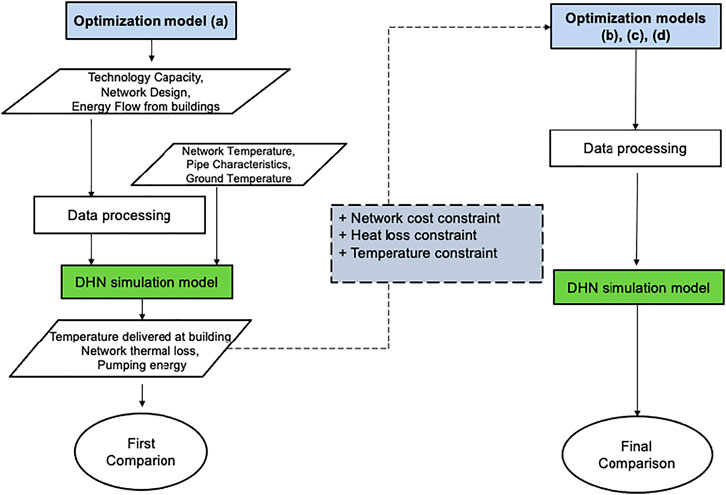
FIGURE 1. General overview of the methodology.

In this section, we introduce at first the existing model formulations, inputs and outputs, and goals of the MILP optimization model 1) and the DHN simulation separately. The key differences in the network representation in both models are summarized in the end. In Comparison of the Mixed‐Integer Linear Programming Model with the District Heating Network Simulation Model and New Mixed‐Integer Linear Programming Model Formulations, the detailed processes of model comparison as first round comparison nd refinement inputs, boundaries, data processes are discussed.

Mixed‐Integer Linear Programming Optimization Model

A MILP optimization model is developed based on the energy hub modeling framework (Geidl and Andersson, 2007). It combines the existing modeling formulations of energy conversion and storage technologies and the thermal networks from (Boran et al., 2016b). The model is treated as a reference model, named as optimization model 1) in this paper. It follows a Mixed‐Integer Linear Programming (MILP) formulation to optimize complex linear problems. The model aims to simultaneously optimize the sizes of technologies and the DHN layouts and their operation to minimize both costs and carbon emissions.

Figure 2 presents the candidate conversion and storage technologies and the interactions with the grid and the DHN at each building in the district. Selected technologies include a natural gas boiler (NB), a biomass boiler (BB), a combined heat and power engine (CHP), a ground source heat pump (GSHP), photovoltaic panels (PV), solar thermal panels (ST), thermal storage tank (TES) and batteries. These technologies are either already present in the Swiss energy system or are considered to be included in the future to meet the goals of the Swiss Energy Strategy. Additionally, buildings can purchase electricity from the electricity grid at a retail price when needed and can sell surplus electricity to the grid at the feed-in tariff. The model formulation of the thermal networks follows the paper by Morvaj et al. (Boran et al., 2016a) and is given in Thermal network constraints. Every building connected to the thermal network is treated as a prosumer, which can either act as a heat source or as a heat sink during operation of the network. Additionally, every building can install heating technologies at the building level, to fulfill its heating demand partially or entirely, and export surplus heat through the network, or receive heat from other neighbor buildings if the network is installed.

FIGURE 2

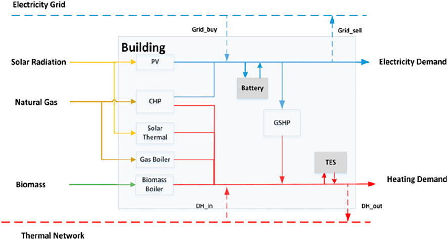
FIGURE 2. Candidate set of energy technologies and energy flow for the D-MES at each building.

The general formulation of the MILP model is a mathematical formulation with equality and non-equality constraints, including predefined parameters and decision variables (both continuous and binaries variables), which specify the design and operation of the system. The model requires input on buildings hourly energy demand (space heating, domestic hot water, and electricity), renewable energy potentials (e.g., solar irradiation), technology operational characteristics (such as operating efficiencies of specific technologies) and local costs information of different energy carriers and technologies.

Objective Function

The objective of the model is to minimize both the Equivalent Annual Cost (EAC) and total carbon emissions of the D-MES. For multi-objective optimization problems in linear programming, the epsilon constraint method (Haimes et al., 1971) is commonly used. In this case, by applying the epsilon constraint method, the minimization of the EAC is formulated as the primary objective function with the set of Eqs. 1–4. The second objective, the total carbon emission, is formulated as an inequality constraint, shown in Eq. 5, with an upper bound known as ${\epsilon }_i$, representing the highest carbon emission the system is constrained. By reducing the limit CO₂ value ${\text{CO}}_{2,\text{limit}}$ in each optimization run, a series of Pareto optimal solutions are generated, which includes the design and operation pattern, thus representing the trade-off between the two conflicting objectives.

$\begin{array}{c}\min \text{EAC}={\text{Cost}}_{\text{inv}}+{\text{Cost}}_{\text{op}}\end{array}(1)$

$\begin{array}{c}{\text{Cost}}_{\text{inv}}={\displaystyle \sum _i{\displaystyle \sum _m{\text{CRF}}_m\cdot \left({\text{LC}}_m\cdot {\text{Cap}}_{i,m}+{\delta }_{i,m}\cdot {\text{FC}}_m\right)}}+{\displaystyle \sum _{i,j}{\text{CRF}}^{\text{pipe}}\cdot {\text{LC}}^{\text{pipe}}\cdot l_{ij}\cdot {\delta }_{ij}^{\text{pipe}} \forall i,j,m,t}\end{array}(2)$

$\begin{array}{c}{\text{Cost}}_{\text{op}}={\displaystyle \sum _i{\displaystyle \sum }_t}\left(c^{\text{biomass}}\cdot I_{i,t}^{\text{biomass}}+c^{\text{gas}}\cdot I_{i,t}^{\text{gas}}\right)+c^{\text{el}}\cdot P_{i,t}^{\text{buy}}-c^{\text{FIT}}\cdot P_{i,t}^{\text{sell}} \forall i,t\end{array}(3)$

$\begin{array}{c}{\text{CRF}}_m=\frac{r\times {\left(1+r\right)}^{N_m}}{{\left(1+r\right)}^{N_m}-1} \end{array}(4)$

$\begin{array}{c}{\text{CO}}_2\text{ emissions} : {\displaystyle \sum _i{\displaystyle \sum _t{\text{CF}}^{\text{gas}}.I_{i,t}^{\text{gas}}+{\text{CF}}^{\text{el}}.\left(P_{i,t}^{\text{buy}}-P_{i,t}^{\text{sell}}\right)\le {\text{CO}}_{2\text{,limit}} \forall i,t}}\end{array}(5)$

The Equivalent Annual Cost (EAC) includes the yearly operational costs $\left({\text{Cost}}_{\text{op}}\right)$ for fuels (biomass, natural gas), cost of buying electricity from the grid, and the revenue from selling electricity to the grid (negative cost). Additionally, amortized investment costs $\left({\text{Cost}}_{\text{inv}}\right)$ of all generation and storage technologies and the thermal network are included.

The cost function of each technology m is constructed by a linear term $\left({\text{LC}}_m\right)$concerning the installed capacity plus a fixed-term ($\left({\text{FC}}_m\right)$) once the technology is installed. ${\text{Cap}}_{i,m}$ is a continuous decision variable representing the installed capacity for technology m at each building i. CRF is the Capital Recover Factor for each technology, accounting the lifetime of the technology $N_m$, and the local interest rate $r$. The investment cost of the thermal network is expressed as a linear function depending on the length of the network between buildings $l_{ij}$. $\delta$ is a binary decision variable defining whether to install a specific technology (generation, storage, or whethertwo buildings should be connected).

The total carbon emissions of the D-MES account for the yearly operational CO₂ emissions of all energy carriers. If electricity is sold to the grid, the resulting CO₂ emissions are deducted. CF represents the carbon emission factor for fuels and electricity. In this study, embodied emissions of different technologies and fuels are not taken into account. Therefore, biomass and PV electricity is considered as carbon-free.

Energy Balance Constraints

For each building i, the energy balance for heat and electricity is formulated as equality constraints shown in Eqs. 6, 7.

The hourly electricity demand is covered by the electricity grid, through discharging the batteries or other electricity-generating technologies (PV and CHP):

$\begin{array}{c}{L}_{i,t}^{\text{el}}=P_{i,t}^{\text{PV}}+P_{i,t}^{\text{CHP}}+P_{i,t}^{\text{buy}}-P_{i,t}^{\text{GSHP}}-P_{i,t}^{\text{sell}}+P_{i,t}^{\text{bat,discha}}-P_{i,t}^{\text{bat,cha}} \forall i,t\end{array}(6)$

For each building i, the heat demand is met by energy from the thermal network (from other building j), through discharging of the TES, or local heating technologies (gas boilers, biomass boilers, CHP, ST panels, and GSHP):

$L_{i,t}^{\text{heat}}=P_{i,t}^{\text{GB}}+P_{i,t}^{\text{ST}}+P_{i,t}^{\text{BB}}+P_{i,t}^{\text{CHP}}\cdot \text{HER}+P_{i,t}^{\text{GSHP}}\cdot \text{COP}+P_{i,t}^{\text{TES,discha}}-P_{i,t}^{\text{TES,cha}}+{\displaystyle \sum _j\left(\left(1-{\text{ls}\cdot \text{l}}_{ji}\right)\cdot q_{ji,t}^{\text{pipe}}-q_{ij,t}^{\text{pipe}}\right) \forall i, t } (7)$

In these equations, $L_{i,t}^{\text{el}}$ and $L_{i,t}^{\text{heat}}$are electricity and heat load required by the building i at the time step t.$P_{i,t}^{\text{PV}}$ and $P_{i,t}^{\text{CHP}}$ are electricity from PV and CHP. HER is the heat to electricity ratio of CHP. $P_{i,t}^{\text{GSHP}}$ is the electricity consumed from GSHP. COP is the coefficient of performance for the GSHP.$P_{i,t}^{\text{buy}}$ and $P_{i,t}^{\text{sell}}$ are electricity bought and sold to the grid. $P_{i,t}^{\text{GB}}$, $P_{i,t}^{\text{ST}}$, $P_{i,t}^{\text{BB}}$, $P_{i,t}^{\text{GSHP}}$ are heat output from the heating technologies. $P_{i,t}^{\text{bat,discha}}$, $P_{i,t}^{\text{bat,cha}}$ , $P_{i,t}^{\text{TES,discha}}$, $P_{i,t}^{\text{TES,cha}}$ are discharging and charging energy from storage technologies (Battery and TES).

For the thermal network, $q_{ji,t}^{\text{pipe}}$ represents the heat flow out from building j to building i. $ls$ is a constant heat loss coefficient per pipe length. $l_{ji}$ represents pipe length between building j and i.

Thermal Network Constraints

The thermal network layout and its operation is defined by the following constraints and then translated into mathematical formulations.

Heat can only be exchanged between buildings that are connected by DHN

$\begin{array}{c}{q}_{ij,t}^{\text{pipe}}\le M\cdot {\delta }_{ij}^{\text{pipe}} \forall i,j,t\end{array}(8)$

where ${\delta }_{ij}^{\text{pipe}}$is a binary variable which indicates whether a pipe between building i and building j is installed or not. $q_{ij,t}^{\text{pipe}}$ is the heat delivered by the pipe from building i to j.

The thermal network is modeled as bi-directional, where energy flow can travel in both directions at different time steps. However, at each time step, only one direction is allowed.

$\begin{array}{c}{\delta }_{ij,t}^{\text{pipe,ope}}+{\delta }_{ji,t}^{\text{pipe,ope}}\le 1\forall i,j,t\end{array}(9)$

where ${\delta }_{ij,t}^{\text{pipe,ope}}$ is a binary variable that defines the operational direction of pipe at time step t.

In the heat energy balance equation (Eq. 7), the heat loss through the network is represented as a linear loss function depending on the length of the pipe.

$\begin{array}{c}\Delta q_{ij,t}^{\text{pipe}}=ls\cdot l_{ij}\cdot q_{ij,t}^{\text{pipe}} \forall i,j,t\end{array}(10)$

Other Model Specifications

As the focus of this paper is on modeling of DHN and to study the effectiveness of its representation at different levels of complexity, only the network constraints are discussed here. Detailed mathematical formulations of other technologies are given in Supplementary Appendix A. The MILP optimization model is programmed in Pyomo, which is an open-source tool for modeling optimization applications in Python. Gurobi optimizer is used for solving the MILP problem. The models were run in parallel with 4 cores and 16 GB of RAM on Euler, an ETH computer cluster. A MIP Gap of 1% is set for all models as an optimality stopping criterion. All relevant technical and economic parameters and coefficients used in the model are given in Supplementary Appendix B.

District Heating Network simulation model

To investigate the operational performance of the network in terms of heat losses, pumping energy, and temperature performance, a thermal network simulation model (DHN model), which was developed previously by the authors (Wang et al., 2021), is used for comparison.

The DHN model was developed in Matlab as a multi-time step steady-state thermal-hydraulic model. It can assess the operational performance of thermal networks with distributed energy sources at different locations, which can act as prosumers to the network. The workflow of the DHN model is displayed. The network model is formulated by graph theory, where each node denotes one building and each edge denotes the connection pipe. Distribution pumps are located at each building for pumping the heat flow from the building to the network. For a given network layout, the design of the pipes is conducted by selecting the appropriate pipe sizes. Once the pipes are designed, a hydraulic model is used to calculate the hydraulic flow and pressure drop along the pipeline. A thermal model is constructed to calculate the temperature distribution within the network at each simulation time step under steady-state conditions. The detailed modeling process and relevant equations of components are given in Wang et al. (Wang et al., 2021). In the following paragraphs of the current paper, three specific aspects are discussed which highlight differences in the thermal network representation between the MILP optimization model 1) and the DHN model.

Pipe Design

The design of the piping network is a complex process. Besides the length of pipes, it involves the selection of pipe materials (e.g., steel or plastic), pipe design (e.g., single pipe, twin-pipe), and different diameters in different sections of the network, which is highly depending on the design temperature level of the network, target pressure loss, allowable flow speed of certain pipe types and the operation strategies of the network. All these factors influence the final costs of the network and the overall energy performance.

Energy flows within the pipes are restricted to a maximum allowable speed$v_{\max }$ of 2 m/s. The inner diameter is calculated as a function of the maximum flow rate $\max \left({\dot{m}}_{ij,t}\right)$ in the pipe, water density, and the maximum allowable speed $v_{\max }$ as:

$\begin{array}{c}{d}_{ij}=\sqrt{\frac{4\cdot \max \left({\dot{m}}_{ij,t}\right)}{\pi \cdot \rho \cdot v_{\max }}}\end{array}(11)$

As a result, the total cost of the piping network is estimated according to the pipe design (nominal diameter), including trench costs and piping costs (Nussbaumer and Thalmann 2016).

Pump Design and Pumping Energy

Individual pumps are designed to be located at each building. They are used to overcome the distribution pressure losses along the network. In the model, the pressure drop along the pipe has a quadratic correlation concerning the mass flow rate according to the Darcy Weisbach equation shown in Eq. 12 at every time step during operation.

$\begin{array}{c}\Delta P_{ij}=f_D\cdot \frac{8l_{ij}}{\rho \cdot {\pi }^2\cdot d_{ij}^5}\cdot {\dot{m_{ij}}}^2\end{array}(12)$

where $f_D$ is the friction factor, which is highly dependent on the flow regime (laminar flow or turbulent flow), the relative roughness of the pipe$\epsilon$ and the inner pipe diameter $d_{ij}$.

For each distributed pump, the pumping power is calculated by Eq. 13.

$\begin{array}{c}{\dot{Q}}_{\text{pump},i}=\frac{\Delta P_i\cdot {\dot{m}}_{si} }{\rho \cdot {\eta }_m\cdot {\eta }_s}\end{array}(13)$

where $P_i$ is the pressure difference derived between supply and return pipelines for buildings providing heat to the network; ${\dot{m}}_{si}$ is the flow rate passing by the pump;${\eta }_m \text{and }{\eta }_s$ are constant values for isentropic and mechanical pump efficiency, respectively.

Temperature Level and Heat Loss

The temperature drop along every single pipe in the flow direction is calculated with Eq. 14. It is dependent on the ground temperature$T_g$, the mass flow rate ${\dot{m}}_{ij}$ along with the pipeline, pipe thermal transfer coefficient $k_{ij}$and pipe length $l_{ij}$.

$\begin{array}{c}{T}_{\text{pipe,out}}=T_g+\left(T_{\text{pipe,in}}-T_g \right)\cdot e^{-\frac{k_{ij}\cdot l_{ij}}{\dot{m_{ij}}\cdot c_p\text{cp}}}\end{array}(14)$

The heat loss along the supply pipeline is then computed as:

$\begin{array}{c}{q}_{ij}={\dot{m}}_{ij}\cdot c_p\cdot \left(T_{\text{pipe,in}}-T_{\text{pipe,out}}\right)\end{array}(15)$

Detailed values used in the DHN model for the pipe costs and other parameters are given in Supplementary Appendix C.

Summary of Thermal Network Parameters in Both Models

The MILP model and the DHN simulation model incorporates different sets of parameters and operational variables in the thermal network representation. This includes the costs (economic impact), pumping energy, and heat losses (energy performance). These variables are summarised in Table 1.

TABLE 1

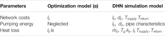
TABLE 1. Summary of key parameters used in the optimization model 1) and the DHN simulation model.

Case Study and Input Parameters

A case study is selected and introduced in this section. The case study district is located in the city of Zurich in Switzerland and consists of 6 residential buildings. Figure 3 shows the 2-D footprints of the buildings in ArcGIS 1) and an image of the selected solar roof area 2) from the Sonnendach database provided by the Swiss Energy Department (Bundesamt für Energie BFE, 2013). The building construction years range from 1900 to 2004. It is assumed that none of them has been retrofitted. The total conditioned area of all buildings is 16103 m².

FIGURE 3

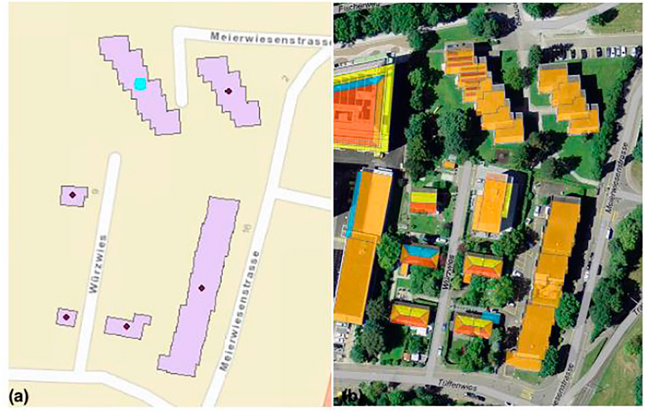
FIGURE 3. ArcGIS 2D footprint (A) and selected roof area with high solar potentials in orange (B) of buildings in the case study district.

Building Energy Demands

To design and operate the D-MES of the case study district with the MILP model, the hourly energy demand of each building is required as an input. The CESAR tool (Combined Energy Simulation and Retrofitting) (Wang et al., 2018) is used for computing the building energy demands, including electricity, space heating, and domestic hot water. It is an urban scale building simulation tool, which uses EnergyPlus (NREL, 2015) as a simulation engine. Occupancy schedules representing different user behavior is from the Swiss SIA norm (SIA, 2016). Other necessary inputs of building information such as building age, building type are taken from the building and apartment registry (“Gebäude und Wohnungregister”) data (BFS, 2013). Inputs on the building’s geometries are taken as 2.5D GIS data from the Swiss Federal Office of Topography (Swisstopo, 2016).

Since the optimization problem considers a full year time horizon at an hourly resolution, the problem is computationally intractable. Therefore, a temporal aggregation based on the typical day approach is used to reduce computational time. It is an effective approach that has been widely used by many design optimization problems, for example, in (Domínguez-Muñoz et al., 2011; Marquant et al., 2017). The number of typical days is selected by minimizing two temporal clustering quality indicators, the error in the load duration curve (ELDC) and the Davies-Bouldin index (Davies and Bouldin, 1979). The Davies-Bouldin index is the ratio of the intra-cluster dispersions to the inter-cluster distance. For the case study district, these two indicators are calculated and shown in Supplementary Figure 1. Ten typical days are selected as a trade-off between the ELDC and the DB index. In total, 13 days are then used, including these 10 days, plus one peak heating, one peak cooling, and one peak electricity demand day. To examine the accuracy of the typical-days approach, the heating demand error in the load duration curve is plotted in Supplementary Figure 1 2) for the anchor building, which is defined as the building with the highest annual heat-demand (Marquant et al., 2015). The red line represents the full-year heating demand simulation results. The blue line is the reconstituted yearly result based on the typical-days representation. Supplementary Figure 2 displays the simulated results of the hourly heating (left) and electricity demand (right) for each building for the 13 typical days. The yearly heating and electricity demand for the district pertains to 1.87 GWh and 0.81 GWh respectively.

Solar Potential Within the Case Study

The hourly solar irradiation profile is obtained from a local weather station and adjusted to the available roof area of all buildings. Data for the available solar roof area on each building is obtained from the Sonnendach database provided by the Swiss Energy Department (Bundesamt für Energie BFE, 2013).

Comparison of the Mixed‐Integer Linear Programming Model with the District Heating Network Simulation Model

In this section, we compared the results from the MILP model, and verified them with the District Heating Network simulation model in three aspects: the network costs, the pumping energy and the thermal performance of the network (as the shown in Figure 1). This process is demonstrated with the case study district discussed in the previous section.

Figure 4 shows Pareto optimal solutions resulting from the MILP optimization model (a), for the objectives total GHG emissions and equivalent annual costs per specific conditioned area. Pareto point (PP) 1 on the bottom-right represents the cost-optimal solution and Pareto point 6 on the top-left represents carbon emission optimal solution. The four Pareto points in between are intermediate solutions by applying the epsilon constraint method to reduce carbon emission targets gradually by 20% starting from the cost-optimal solution. Heating and storage technologies, which are installed at each building for each Pareto optimal solution are shown in Figure 5.

FIGURE 4

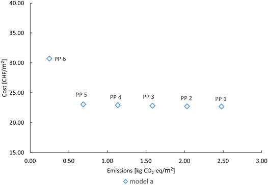
FIGURE 4. Pareto fronts of specific emissions vs. equivalent annual costs.

FIGURE 5

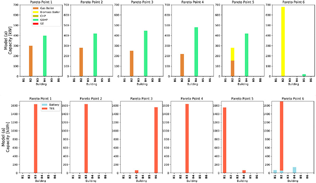
FIGURE 5. Heating technologies (top) and storage technologies (bottom) size installed at each building for all Pareto optimal solutions.As here, the main focus is the comparison of the thermal network design and performances from both models. Detailed results of system-level design and analysis of other technologies are further discussed in Results and discussion for optimization model comparison.

The technology capacity, the installation locations, and the optimal network layout (whether buildings should be connected to the network or not) are results from the MILP models for optimal Pareto solutions. We then processed this information on system design and operational conditions as input to the district heating network simulation model. The thermal network pipes are designed accordingly for the layout for each optimal solutions. The network operational performances are then simulated with the DHN simulation model.

As the simulation model requires more design and operational input than the MILP model is capable of providing, further assumptions are made to design and simulate the network using the DHN simulation model:

The designed supply and return temperatures are assumed to be 70 and 30°C, respectively.

The mass flow rate carried from one building node to the other building node ${\dot{m}}_{ij}$ is approximated in Eq. 16 with a constant temperature difference of $T$ = 40°C controlled at the substation.

$\begin{array}{c}{\dot{m}}_{ij}=\frac{q_{ij}}{\text{cp}\cdot \Delta \text{T}}\end{array}(16)$

The district heating network is a single pipe network. Heat losses along the return pipeline are generally very low; hence they are neglected.

Network Costs

Figure 6 shows the network layout design of the MILP model for all Pareto points solutions. The model suggests that all buildings should be connected to the district heating network in all scenarios and that the shortest path to connect all the buildings is selected in most solutions, except the carbon optimal scenario at Pareto point 6. In this figure, the comparison of annualized investment costs for the MILP optimization model and the DH simulation model is displayed. On average, the assumptions from the optimization model 1) indicate slightly higher costs (around 2%) compared to the DHN simulation model. The piping layout and length are identified by the MILP model, in this regard, the two models use the same input; however, the DHN simulation model additionally sizes the pipe diameter, which causes the difference of approximately 2% in the annualized investment costs between both models.

FIGURE 6

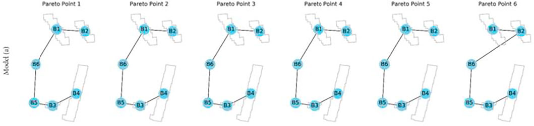
FIGURE 6. Network layout and annualized investment costs in [CHF].

Pumping Energy and Pump Costs

In the optimization model (a), distribution pumps are neglected. As a result, there is no extra electricity consumption or any costs considered regarding the distribution pumps. However, by running the DHN simulation model, we need a specific design capacity for the distribution pumps to obtain the pumping energy. A range of pumps with different capacities (between 1 and 6 kW) is selected for all the Pareto point solutions. The average yearly pumping energy is 3.63 MWh, which takes up only 0.47% of the yearly total electricity demand for the case study district. The equivalent annual investment cost of pumps is relatively low, which does not play a significant role in the decision-making process for the system-level design and district heating network design, resulting in higher computational costs. Therefore, we conclude that pumping energy and extra pump costs are negligible in the MILP model for this small case study.

Heat Loss

Hourly heat losses are compared for both models. Figure 7 shows one exemplary comparison for the scenario with 0.69 kg CO₂-eq/m² (Pareto point 5). For the whole year, the overall heat loss is underestimated by the MILP model compared to the DHN simulation results. On an hourly basis, there is a significant discrepancy, especially during low heating demand hours (typical day 1, day 4, day 12, and day 13). As heat loss is only modeled as a constant percentage per pipe length to the total energy delivered by the network, the operational performance including the non-linear behavior in the heat loss approximation of the district heating network, is not reflected in the optimization model.

FIGURE 7

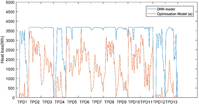
FIGURE 7. hourly network heat loss for typical days (TPD).

Temperature Sufficiency

The DHN simulation model, which takes the supply system design from the optimization model as an input, can simulate the temperature distribution within the network, whereby a design supply temperature of 70°C is considered. If district heating networks are used to supply buildings with both space heating and domestic hot water, a critical delivered temperature of 55°C at the building is required at the building site to prevent the risk of legionella growth. Figure 8 shows the temperature delivered to each building during the simulation period for the same scenario with 0.69 Kg CO₂-eq/m² (Pareto point 5). The red horizontal line indicates the critical temperature of 55°C. Results show that the required temperature is insufficient for some of the buildings.

FIGURE 8

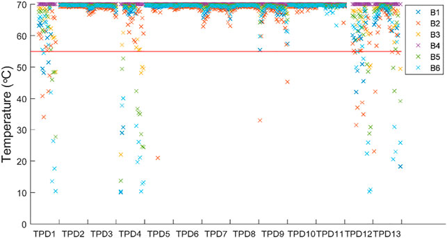
FIGURE 8. Temperature delivered at the buildings during the simulation period.

We can observe that insufficient temperatures mainly occur during low heating demand days (typical day 1, day 4, day 12, and day 13). To guarantee sufficient operation of the thermal network during these periods, a bypass valve should open to increase the mass flow circulating in the pipeline to improve the temperature drop, thus resulting in higher energy consumption than the buildings need. In the current formulation of the network representation in the model (a), this operational issue is not addressed.

New Mixed‐Integer Linear Programming Model Formulations

To make a better approximation of the network representation in the MILP model, and to resolve discrepancies between the optimizations and the DHN simulation model, new network constraints have been implemented based on the original MILP model: optimization model (a).

The following assumptions are additionally made to derive the new thermal network constraints, which are consistent with the DHN simulation model setup:

The designed supply temperature $T_{\text{supply}}$ and return temperature $T_{\text{return}}$ are 70°C and 30°C respectively.

The mass flow rate carried from one building node to the other building node ${\dot{m}}_{ij}$ is approximated in Eq. 16, with a constant temperature difference of $T$ = 40°C controlled at the substation.

• The district heating network is a single pipe network. Heat losses along the return pipeline are neglected.

• The costs of the pumps and pumping energy are neglected.

• The temperature to be delivered to the consumers should be above the critical delivered temperature at buildings $T_{\text{limit}}$ at 55°C.

Network Cost Constraint

To account for the discrepancy in pipe costs as shown in Network costs, a more accurate definition of network costs is derived. This is done by introducing the new term pipe capacity ${\text{Cap}}_{ij}^{\text{pipe}}$ , which is defined as the maximum energy intensity that the designed pipe is capable of delivering without accounting for heat losses of the pipe.${\text{Cap}}_{ij}^{\text{pipe}}$ is then converted as a function of the designed pipe diameter in the following equation, which combines Eq. 11 and Eq. 16.

$\begin{array}{c}{\text{Cap}}_{ij}^{\text{pipe}}=c_p\cdot \Delta T\cdot \pi \cdot \rho \cdot v_{\max }\cdot {\left(\frac{1}{2}{d}_{ij}\right)}^2\end{array}(17)$

A linear regression of the cost function used in the DHN model concerning the pipe diameter is performed first. Then a piecewise linear approximation is extrapolated to represent the size dependency of the network costs. Supplementary Figure 3 shows the extrapolated cost coefficient as a function of pipe capacity, in comparison to the formulation in the DHN and the optimization model (a).

Then the investment costs of the district heating network, used in the objective function is formulated dependent on the pipe capacity ${\text{Cap}}_{ij}^{\text{pipe}}$ as follows:

$\begin{array}{c}{\text{cost}}_{\text{dhn}}={\text{CRF}}_{\text{dhn}}\times \left[\left(a1+b1{\text{Cap}}_{ij}^{\text{pipe}}\right){\delta }_{1,ij}^{\text{pipe}}+\left(a2+b2{\text{Cap}}_{ij}^{\text{pipe}}\right){\delta }_{2,ij}^{\text{pipe}}\right]\times l_{ij}\end{array}(18)$

$\begin{array}{c}{\text{Cap}}_{ij}^{\text{pipe}}\le {\delta }_{1,ij}^{\text{pipe}}\cdot {\text{Cap}}_{\text{Seg}1}^{\text{pipe}}+{\delta }_{2\text{,ij}}^{\text{pipe}}\cdot M\end{array}(19)$

$\begin{array}{c}{\text{Cap}}_{ij}^{\text{pipe}}\ge {\delta }_{2,ij}^{\text{pipe}} \cdot {\text{Cap}}_{\text{Seg}1}^{\text{pipe}}\end{array}(20)$

$\begin{array}{c}{\delta }_{1,ij}^{\text{pipe}}+{\delta }_{2,ij}^{\text{pipe}}\le 1\end{array}(21)$

where ${\delta }_{1,ij}^{\text{pipe}}\text{and} {\delta }_{2,ij}^{\text{pipe}}$ are binary variables specifying the active line segment in the piecewise linear approximation for the pipe capacity. ${\text{Cap}}_{\text{Seg}1}^{\text{pipe}}$ is the maximum size value for the first segment of the curve. When ${\delta }_{1,ij}^{\text{pipe}}\text{and} {\delta }_{2,ij}^{\text{pipe}}$ are both 0, which forces ${\text{Cap}}_{ij}^{\text{pipe}}$ to be 0 by the constraints, then no pipe connection is installed between node i and j. a1, a2 and b1, b2 are intercepts and slopes of the two segments. Detailed values are given in Table C2 in Supplementary Appendix C.

Heat Loss Constraint

For one single pipe, by combining the assumptions used in Eqs. 14–16, the heat loss is approximated as a function of the heat input $q_{ij}^{\text{pipe}}$ into the network from i to j.

$\begin{array}{c}\Delta q_{ij}=\frac{T_{\text{pipie,in}}-T_g}{\mathrm{\Delta T}}\cdot \left(1-e^{-\frac{k_{ij}\cdot l_{ij}\cdot \Delta T}{q_{ij}^{\text{pipe}}}}\right)\cdot q_{ij}^{\text{pipe}}\end{array}(22)$

For Eq. 22, with the first-order Taylor expansion, when $q_{ij}^{\text{pipe}}$ is relatively big, the heat loss could be linearly interpolated as a function of the pipe length, which results in an approximated representation, as shown in.

$\begin{array}{c}\Delta q_{ij}\approx \left(T_{\text{in}}-T_g\right)\ast k_{ij}\cdot l_{ij}\end{array}(23)$

For each pipe, $T_{\text{in}}$ is assumed to be the designed supply temperature $T_{\text{supply}}$, the temperature cascade along the pipeline is neglected. The thermal transfer coefficient $k_{ij}$ is a property, which depends on the pipe thermal conductivity, the diameter, and the insulation level of the pipes. The correlation of this factor as a function of the pipe diameter chosen in the DHN model is used. A threshold value $q_{ij}^{\text{pipe,threshold}}=k_{ij}^{\text{linear}}{l}_{ij}\left(T_{\text{supply}}-T_g\right)$ is set as a lower bound for the energy input into the district heating network, to avoid that the heat input into the thermal network is smaller than the heat loss along the pipe.

In the DHN simulation model, the thermal transfer coefficient $k_{ij}$ is a linear function of pipe diameter, instead of ${\text{Cap}}_{ij}^{\text{pipe}}$. Therefore, we used linear regression to derive the function between $k_{ij}^{\text{linear}}$ and ${\text{Cap}}_{ij}^{\text{pipe}}$ . Then we obtain the new thermal loss coefficient$k_{ij}^{\text{linear}}=a+b\times {\text{Cap}}_{ij}^{\text{pipe}}$. Detailed values of a and b are given in Supplementary Appendix C.

In the MILP model, the thermal balance equation of model 1) is then reformulated, where the new heat loss function of the network is implemented, as follows:

$L_{i,t}^{\text{heat}}=P_{i,t}^{\text{GB}}+P_{i,t}^{\text{ST}}+P_{i,t}^{\text{BB}}+P_{i,t}^{\text{CHP}}\cdot \text{HER}+P_{i,t}^{\text{GSHP}}\cdot \text{COP}+P_{i,t}^{\text{TES,discha}}-P_{i,t}^{\text{TES,cha}}+{\displaystyle \sum _j\left(\left(q_{ji,t}^{\text{pipe}}-k_{ji}^{\text{linear}}\cdot l_{ji}\cdot \left(T_{\text{supply}}-T_g\right)\right)\cdot {\delta }_{ji,t}^{\text{loss}}-q_{ij,t}^{\text{pipe}}\right)\forall i,j,t}(24)$

$\begin{array}{c}{q}_{ij,t}^{\text{pipe}}\ge {\delta }_{ij,t}^{\text{loss}}\cdot q_{ij,t}^{\text{pipe,threshold}} \forall i,j,t\end{array}(25)$

$\begin{array}{c}{q}_{ij,t}^{\text{pipe}}\le {\delta }_{ij,t}^{\text{loss}}\cdot M\forall i,j,t\end{array}(26)$

where ${\delta }_{ij,t}^{\text{loss}}$ is a binary variable indicating whether $q_{i,j,t}^{\text{pipe}}$is larger than the threshold $q_{ij}^{\text{pipe,threshold}}$ Specifically, ${\delta }_{ij,t}^{\text{loss}}=1$ if $q_{i,j,t}^{\text{pipe}} >q_{ij}^{\text{pipe,threshold}}$; ${\delta }_{ij,t}^{\text{loss}}=0$ if $q_{ij,t}^{\text{pipe}} \le q_{ij}^{\text{pipe,threshold}}$. This is also formulated as a big M constraint in the linear programming method.

Temperature Constraint

In the current version of the MILP model, only heat losses of the pipe are taken into account to represent the thermal behavior of the thermal network. However, simulation results showed that the delivered temperatures at buildings are often not sufficient on most of the summer days when the heat demand is very low. To improve this behavior, minimum heat input to the thermal network is added as a new constraint. $q_{ij}^{\text{pipe,limit}}$ is computed by Eq. 27, whereby the required minimum temperature $T_{\text{limit}}$ is set at 55°C. Additionally, a 5°C safety buffer value is used to counterbalance the effect of temperature cascade along the water stream, where the upstream temperature is assumed as $T_{\text{supply}}$.

$\begin{array}{c}{q}_{ij}^{\text{pipe,limit}} =k_{ij}^{\text{linear}}\cdot l_{ij}\cdot \Delta T\cdot \frac{1}{\lg \left(\frac{T_{\text{supply}}-T_g}{T_{\text{limit}}+5-T_g}\right)}\end{array}(27)$

This constraint is added to the MILP model with the following equation:

$\begin{array}{c}{q}_{ij,t}^{\text{pipe}}\ge {\delta }_{ij,t}^{\text{loss}}\cdot k_{ij}^{\text{linear}}\cdot l_{ij}\cdot (\Delta T)\cdot {\beta }_{\text{limit}} \forall i,j,t\end{array}(28)$

where ${\beta }_{limit} =\frac{1}{\lg \left(\frac{T_{\text{supply}}-T_g}{T_{\text{limit}}+5-T_g}\right)}=5.48$, calculated with the given value in this particular case.

Summary of the Mixed‐Integer Linear Programming Optimization Model Formulations

These three new constraints have been gradually implemented based on the MILP model (a), resulting in three other model versions: model (b-d). The new models are applied to the aforementioned case study district.

Table 2 summarizes the different model versions, including the resulting computational time and number of binaries for each model. We can see that as the model complexity increases, with additional binary variables introduced gradually to model (b-d), the computational time of the models increases significantly by almost 6 times higher in the most complex model 4) compared to the original model (a).

TABLE 2

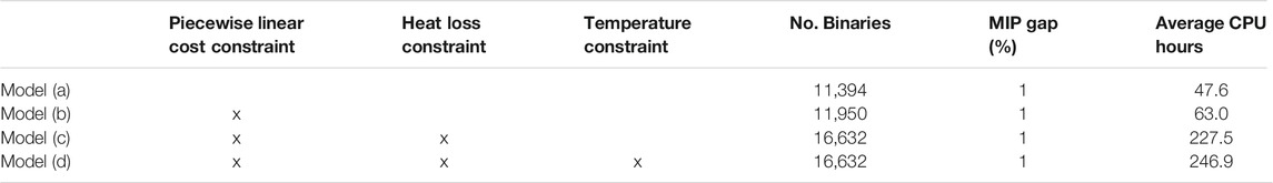
TABLE 2. Summary of MILP model characteristics and executing CPU time.

Results and Discussion for Optimization Model Comparison

In this section, the solutions from the original MILP model 1) and refined model (b-d) are given and detailed results are analyzed and compared.

System Design

Figure 9 shows Pareto optimal points of each optimization model (a-d), in terms of total GHG emissions and costs per specific conditioned area. Solution 1 on the bottom-right represents the minimum cost solution and solution 6 on the top-left represents the minimum CO₂ emission solution. The technology selection for conversion and storage technologies of each Pareto point is shown in Figure 10.

FIGURE 9

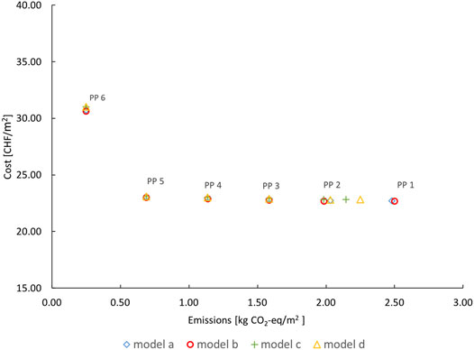
FIGURE 9. Pareto fronts of optimization model (A)-(D).

FIGURE 10

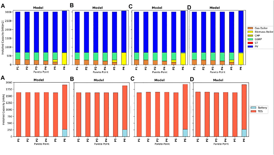
FIGURE 10. Energy conversion technologies capacity and storage technology size for all Pareto optimal solutions from the optimization model (A)-(D).

Figure 9 shows that all 6 Pareto points of the different optimization models 1) to 4) reside at similar locations on the plot. Since emission targets for all points between 2 and 5 are close, also optimal costs do not significantly deviate among the different models, even though different levels of complexity of the thermal network representations are made from the model 1) to model 4) (as described in the methodology, Comparison of the Mixed‐Integer Linear Programming Model with the District Heating Network Simulation Model).

Figure 10 shows that there are only minor differences regarding both technology selection and installed capacities. A general trend in technology selection can be observed, which shows that in the cost-optimal solution, PV panels, heat pump, gas boiler, and thermal storage tanks are chosen. To further reduce the CO₂ emissions, gas boilers are gradually replaced with ground source heat pumps. The carbon optimal solution usually includes a biomass boiler and PV panels, which are installed up to the maximum available roof space. A CHP unit is still too expensive for this small district due to its high investment costs.

Thermal storage tanks are selected in all solutions mainly for two reasons: 1) to cover the peak heating demand together with reduced size of the boiler and 2) to be charged when there’s surplus electricity generated from PV panels together with operating the heat pumps. As the battery is still a very costly technology, it is not considered in most of the solutions, except for the carbon optimal solution.

PV panels are often selected as a cost-effective technology for this particular district, as investment costs are relatively reasonable and potential gains from feed-in tariffs are an economically viable option compared to relying entirely on electricity from the grid. Even though solar thermal panels are given as a potential option, in competing with PV panels for the limited available building roof space, it is never chosen in any of the solutions. This is mainly due to the relatively high price of solar thermal panels in Switzerland. Besides, to decarbonize the heating section, alternative economical solutions are available by using biomass boilers or heat pumps. However, for covering the electricity demand, PV panels are the only available clean technology. Figure 11 shows the installed capacities of PV panels for the 6 buildings corresponding to each Pareto point, from cost-optimal to carbon optimal solutions. Please note, that the same solution for PV panels is obtained from all model versions, as district heating network installation did not make any impact on the design of electrical systems. Results show that in the first 5 Pareto points, buildings 1-4 are fully covered by PV panels utilizing all of the available roof areas. In the last Pareto point, all the buildings are fully covered.

FIGURE 11

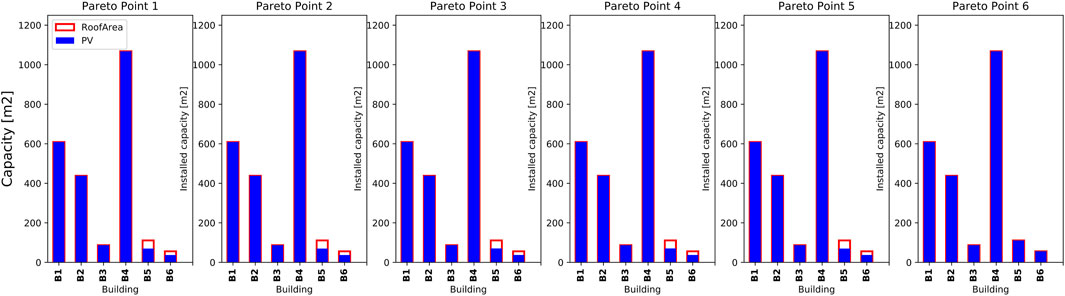
FIGURE 11. installed PV capacities on each building for all Pareto optimal solutions.

Figure 12 and Figure 13 shows installed capacities of energy conversion (for space heating and domestic hot water) and storage technologies respectively for all buildings and model versions. The optimal district heating network layout is also displayed for each solution in Figure 14, whereby the line thickness represents the pipe capacity. Please note that model 1) considers only the pipe length for the network design; therefore, there is no specific design capacity for the pipes.

FIGURE 12

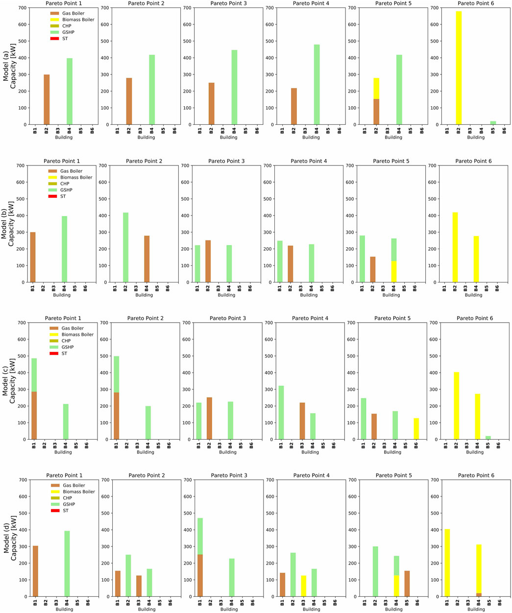
FIGURE 12. Design capacities of heating technologies at each building from the model (A)-(D).

FIGURE 13

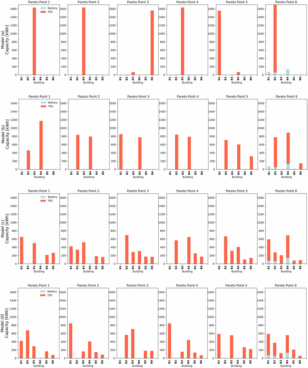
FIGURE 13. Design capacities of storage technologies (TES and Battery) from the model (A)-(D).

FIGURE 14

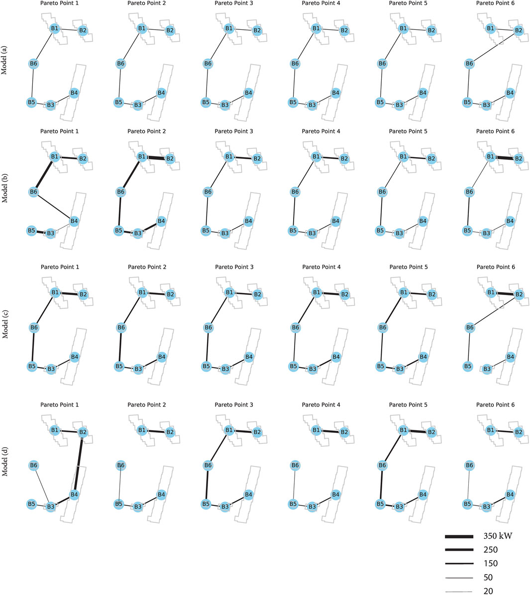
FIGURE 14. Design capacities of storage technologies (TES and Battery) from the model (A)-(D).

When comparing results at the building level, there is a significant change in where and which technologies are installed between the different model versions. Also, the district heating network layout differs among the models. A clear trend is observed by comparing results from the model 1) to (d). In model version (a), big size heating technologies are selected and located in more “centralized” locations, mostly at the biggest energy consumers (which are building 2 and building 4). Heat is then distributed by the thermal network to smaller energy consumers. In the model version (d), multiple small size technologies are selected and are more evenly distributed at multiple buildings’ locations. The same trend is observed for thermal storage technologies. Whereas in model version (a), big thermal storage tanks are installed at one single building, more and more small units are installed in a distributed manner when moving from version 2) to (d).

Regarding the optimal district network layout, both model 1) and 2) suggest that all buildings should be connected. The shortest path is the optimal layout in most of the solutions. More diversity in the network layout is shown in model 3) and (d), indicating that not all buildings need to be connected and even if they are connected, the shortest path may not be the optimal solution in reaching system cost and CO₂ emission optimality.

As explained in the model methodology section, a new capacity based piecewise linear network cost function has been introduced in the model (b), where network investment costs do not only depend on the pipe length, but also the pipe diameters. Optimization results show that this update did not impact the network layout design significantly. This might be because that with this new update of the model, investment costs can be more accurately predicted, however, the overall investment costs for the district heating network only takes up around 2% of the equivalent annual costs of the entire system for this small district, since total investment costs are mainly dominated by the heating technologies and PV panels.

System Operation

Operational results of one exemplary solution for the scenario with 0.69 kg CO₂-eq/m² (Pareto Point 5) from the model 1) and model 4) are shown in Figure 15.

FIGURE 15

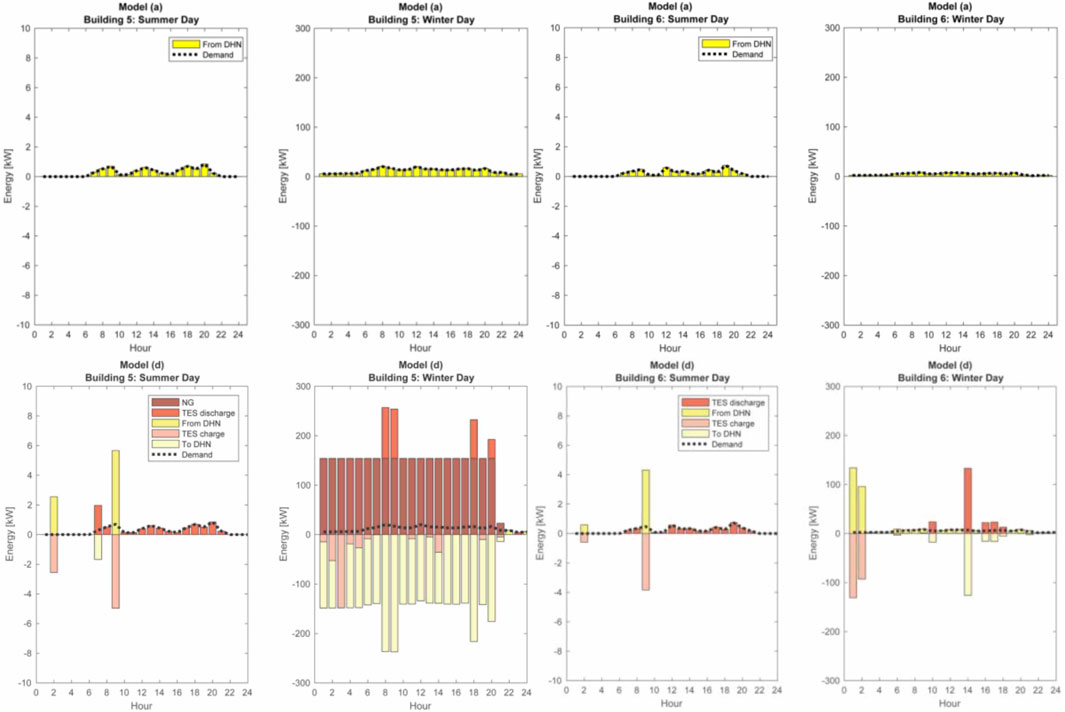
FIGURE 15. Times series of the output of technologies for a typical winter day and a typical summer day for building 5 and 6 from the model (A)(top) and model (D)(bottom).

In this figure, hourly operation over 1 day of installed technologies and the interaction with the district heating network of building 5 and building 6 are shown. Results are given for one typical summer and one typical winter day. As building 5 and 6 are both small energy consumers, which are located at a middle position of the district heat network branch, model 1) gives as an optimal solution that both buildings’ heat demand is covered by the district heating network through heat supplied by heating systems of other buildings. On the contrary, with minimum energy flow constraint added in the model (d), both the optimal design and operation of building 5 and 6 behave differently compared to model (a). As discussed in Temperature sufficiency, insufficient temperature levels occurred during summertime in model version (a). To overcome this issue, the optimization results of the model 4) show that thermal energy storage is installed at both buildings. Additionally, a natural gas boiler is installed at building 5. At a typical summer day, the thermal storage tank is charged within one timestep from the district heating network; the heat is then locally stored and gradually discharged to supply heat to the building. On a winter day, the gas boiler in combination with the thermal storage works as the primary energy source to cover the heating demand locally at building 5 and additionally supplies heat to other buildings through the district heating network. At building 6, only a thermal storage tank is installed. The same behavior pattern is observed during a summer day as in building 5. On a winter day, the thermal storage tank is charged through the district heating network at some time step, and later used to partially cover its heat demand and feed in back to the network to supply heat to other buildings.

The corresponding operational performance of the thermal network of optimization model 1) and 4) is then simulated by the DHN model, using the optimal operation schedules of technologies given from the optimization model. Hourly temperature distribution at all consumer substations is obtained. Figure 16 shows an example the hourly temperature delivered to building 5 and 6 during the simulation period (13 typical days (TPD), 312 h in total) for the same scenario with 0.69 kg CO₂-eq/m² (Pareto point 5) for model 1) and model (d), where the red horizontal line indicates the critical temperature.

FIGURE 16

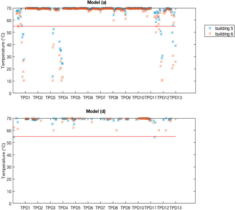
FIGURE 16. Simulation results of temperature delivered at the building with optimal design given by model (A)(top) and model (D)(bottom).

Results show that model 4) heat supply temperatures stay at almost all time steps above the required temperature of 55°C, whereas in the model 1) in many instances, insufficient supply temperatures occur. Due to the update of the model, which takes temperature levels at the substations into account, the system configuration changed between the model versions. In this case, thermal storage tanks are installed and operated during summer locally at the consumer, which avoids an inefficient operation of the network. This could tremendously improve the operational performance of the district heating network.

To quantify this behavior, the percentage of hours of the year with insufficient supply temperatures delivered to the buildings is calculated and shown in Figure 17 for all model versions. For each typical day, the number of hours is counted when the temperature delivered to the buildings is lower than the 55°C limit. The resulting values of the typical days are then scaled up to the whole year.

FIGURE 17

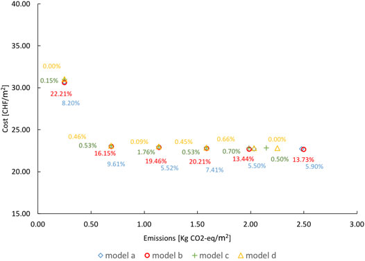
FIGURE 17. Pareto points of optimization model (A)-(D) with the percentage of insufficient temperature supply indicated.

The results show that for the model (a), the heat supply temperature is insufficient for 5.5–9.61% time of the year for the various scenarios. By implementing a new cost function in the model (b), which better approximates the network investment costs, the problem of insufficient heat supply temperatures even increases during operation. In model 3) and model (d), this issue is gradually improved with the integration of a new heat loss constraint and temperature limit constraint, thus resulting in better design and operational strategies. Model 4) shows in this case, a reduced insufficient heat supply temperature rate of below 0.66% over a year for all Pareto solutions.

Conclusion

This paper investigates different modeling methods of thermal networks under the scope of the optimal design and operation of D-MES for urban districts. A common optimization approach for D-MES is based on a Mixed‐Integer Linear Programming method. To guarantee model linearity and to limit computational expenses, thermal networks are usually represented through a simple fixed percentage of heat loss per pipe length and a fixed investment cost per pipe length. Neither the dependence of the pipe selections from different designs (e.g., diameter, insulation levels) nor the thermal-dynamics of heat flow along the pipeline during operations are considered.

We investigated the effectiveness of this representation of thermal networks in the MILP model formulation by comparing it to a more detailed thermal-hydraulic network simulation model, which can address the non-linear behavior in the design and operational performance of the thermal network. Results of the case study show that:

• The network costs are slightly underestimated by the original MILP model.

• The required pumping energy is small enough to be negligible in the MILP model.

• Heat losses are underestimated periodically in the MILP model, especially during low heating load periods in summer days.

• During some periods of the year, buildings heated by the thermal networks do not receive a sufficient temperature level at above 55°C.

To bridge the discrepancies, further refinements are made to improve the current MILP model formulations by adding new constraints with a new piece-wise linear cost constraint, a heat loss constraint, and a minimum heat distribution constraint. As a result, more binary variables are introduced, which increases the solving time by 6 times. The refined more complex model prescribes similar optimal technology selections at the district level, nevertheless, technologies are suggested to be installed more distributed at the building side together with storage tanks. During operation, small heating demands are covered by the local thermal storage tanks, which are charged from the district heating networks. Consequently, the temperature insufficiency which occurred in the original MILP model improved significantly. Overall, for the demonstrated small case district, it reveals that the state-of-art MILP-model with simplified network representation suffices for the optimal selection and sizing of most suitable technologies at the district level. However, to address operational issues such as temperature sufficiency and heat loss, a more sophisticated model is needed. In general, results suggest that the optimal design solution in regard to costs and carbon emissions doesn't follow a clear pattern. For some Pareto-optimal solutions not all buildings are connected and if they are connected, then the shortest route is not always selected as the optimal network layout. Furthermore it is found that parameters such as the designed pipe capacity, the selection of heat generation and storage technology are vital criteria in the design space, whereas the pumping energy during operation doesn't play an important role in the design phase of the network.

Even though these findings are case-specific, the methodology developed could be applied to areas of different complexity (such as different building types, sizes of the district, etc.). In this paper, we tested the methodology on a small case study of 6 buildings due to the computational complexity with a large number of decision variables. Resulting limitations that were observed are discussed in the previous section. It can be assumed that for larger districts that are equipped with a longer network, the impact of network costs would be more pronounced. A potential underestimation of the heat losses from the returning pipes could also have additional impact. In addition, due to longer transmission distance, the impact of temperature drop along the pipelines, that results in a temperature insufficiency issue will become more significant. As the inaccuracy in the heat loss linear approximation in the simplified MILP model mostly occurs during low demand periods in summer, this effect might be counter-balanced for a district with higher heating demands.

Whether network costs or the impact of pumping energy would change for other case studies, need to be tested with a more comprehensive analysis with varying district sizes, heat demand densities, and climatic conditions. Additionally, other options of DHN network configurations (e.g., loop networks) and different temperature levels (e.g., low temperature, ultra-low temperature networks) could be investigated with this approach, to come to more general findings and recommendations.

For this case study, embodied emissions of the different technologies are currently not included. The reason for this choice was that on the one hand, the Swiss energy strategy 2050 is based on non-life cycle emission values, and on the other hand, current literature lacks detailed data for accounting embodied emissions of thermal networks including piping material and construction in Switzerland. This choice might impact the overall decisions on optimal technology selections and the DHN network design. Besides, due to the computational complexity, we only considered daily storage technologies. An interesting addition to the present work would be the inclusion of seasonal storage technologies such as borehole storage. Finally, a common issue for simulation and optimization studies is that results are sensitive to the input data employed. The overall goal of this paper is, to showcase the process of investigating modeling methodologies of DHN representations for D-MES and to demonstrate the outcome for a specific case. However, an uncertainty and sensitivity analysis regarding the critical input parameters would be needed, which is out of the scope of this paper, to derive more general conclusions for the appropriate level of detail in the DHN representation.

Data Availability Statement

The raw data supporting the conclusions of this article will be made available by the authors, without undue reservation.

Author Contributions

Conceptualization: DW, JM and KO; Methodology and model development: DW, XL and JM; Formal analysis and data curation: DW and XL; Visualization and writing original draft: DW and XL; Review and Editing: DW, XL, JM, KO and JC; Supervision: JC and KO; All authors have read and agreed to the published version of the manuscript.

Funding

This research has been financially supported by the Swiss National Science Foundation (SNSF) under the RePoDH project (Renewable powered district heating networks Nr.165978).

Conflict of Interest

The authors declare that the research was conducted in the absence of any commercial or financial relationships that could be construed as a potential conflict of interest.

Supplementary Material

The Supplementary Material for this article can be found online at: https://www.frontiersin.org/articles/10.3389/fenrg.2021.668124/full#supplementary-material

References

BFS (2013). Bundesamt Für Statistik, Gebäude Und Wohnungsstatistik (GWS) 2013.

Boran, Morvaj., Evins, Ralph., and Jan, Carmeliet. (2016a). Optimising Urban Energy Systems: Simultaneous System Sizing, Operation and District Heating Network Layout. doi:10.1016/j.energy.2016.09.139

CrossRef Full Text

Boran, Morvaj., Evins, Ralph., and Jan, Carmeliet. (2016b). Optimization Framework for Distributed Energy Systems with Integrated Electrical Grid Constraints. Appl. Energ. 171, 296–313. doi:10.1016/j.apenergy.2016.03.090

CrossRef Full Text | Google Scholar

Brange, L., Englund, J., and Lauenburg, P. (2016). Prosumers in District Heating Networks - A Swedish Case Study. Appl. Energ. 164, 492–500. doi:10.1016/j.apenergy.2015.12.020

CrossRef Full Text | Google Scholar

Bundesamt für Energie BFE (2013). n.d. “Sonnendach.” Available at: https://www.uvek-gis.admin.ch/BFE/sonnendach/.

Davies, D. L., and Bouldin, D. W. (1979). A Cluster Separation Measure. IEEE Trans. Pattern Anal. Mach. Intell. PAMI-1 (2), 224–227. doi:10.1109/TPAMI.1979.4766909

PubMed Abstract | CrossRef Full Text | Google Scholar

Domínguez-Muñoz, F., Cejudo-López, J. M., Carrillo-Andrés, A., Gallardo-Salazar, M., and Gallardo-Salazar, Manuel. (2011). Selection of Typical Demand Days for CHP Optimization. Energy and Buildings 43, 3036–3043. doi:10.1016/j.enbuild.2011.07.024

CrossRef Full Text | Google Scholar

Fazlollahi, S., Becker, G., and Maréchal, F. (2014). Multi-Objectives, Multi-Period Optimization of District Energy Systems: III. Distribution Networks. Comput. Chem. Eng. 66, 82–97. doi:10.1016/j.compchemeng.2014.02.018

CrossRef Full Text | Google Scholar

Fonseca, J. A., Nguyen, T.-A., Schlueter, A., and Marechal, F. (2016). City Energy Analyst (CEA): Integrated Framework for Analysis and Optimization of Building Energy Systems in Neighborhoods and City Districts. Energy and Buildings 113, 202–226. doi:10.1016/j.enbuild.2015.11.055

CrossRef Full Text | Google Scholar

Geidl, M., and Andersson, G. (2007). In 2007. IEEE Lausanne POWERTECH, 1398–1403. doi:10.1109/PCT.2007.4538520 Optimal Coupling of Energy Infrastructures. Proceedings.

CrossRef Full Text | Google Scholar

Haimes, Y., Ladson, L. S., and Wismer, D. A. (1971). On a Bicriterion Formulation of the Problems of Integrated System Identification and System Optimization. IEEE Trans. Syst. Man, Cybernetics SMC- 1, 296–297. doi:10.1109/TSMC.1971.4308298

CrossRef Full Text | Google Scholar

Hassine, Ilyes. Ben., and Eicker, Ursula. (2013). Impact of Load Structure Variation and Solar Thermal Energy Integration on an Existing District Heating Network. Appl. Therm. Eng. 50 (2), 1437–1446. doi:10.1016/j.applthermaleng.2011.12.037

CrossRef Full Text | Google Scholar

IEA (2018). Energy Policies of IEA Countries. Switzerland. 2018 Review Available at: www.iea.org/t&c/.

Jakob, M., Kallio, S., Otto, W., Nägeli, C., Bolliger, R., and Von Grünigen, S. (2015). INSPIRE-tool. TEP Energy GmbH & Econcept AG. http://www.inspire-tool.ch.

Google Scholar

Li, H., and Svendsen, S. (2013). District Heating Network Design and Configuration Optimization with Genetic Algorithm. J. Sustain. Dev. Energy Water Environ. Syst. 1 (14), 291–303. doi:10.13044/j.sdewes.2013.01.0022

CrossRef Full Text | Google Scholar

Liu, X., Jenkins, N., Wu, J., and Bagdanavicius, A. (2014). Combined Analysis of Electricity and Heat Networks. Energ. Proced. 61, 155–159. doi:10.1016/j.egypro.2014.11.928

CrossRef Full Text | Google Scholar

Lund, H., Arler, F., Østergaard, P. A., Østergaard, P., Hvelplund, F., Connolly, D., et al. (2017). Simulation versus Optimisation: Theoretical Positions in Energy System Modelling. Energies 10 (7), 1–17. doi:10.3390/en10070840

CrossRef Full Text | Google Scholar

Marquant, J. F., Akomeno, O., Orehounig, K., Evins, Ralph., and Jan, Carmeliet. (2015). Application of Spatial-Temporal Clustering to Facilitate Energy System Modelling. In 14th Conference of International Building Performance Simulation Association, Hyderabad, India, Dec 7–9, 2015. Conference Proceedings, 551–558.

Google Scholar

Marquant, J. F., Evins, R., Bollinger, L. A., and Carmeliet, J. (2017). A Holarchic Approach for Multi-Scale Distributed Energy System Optimisation. Appl. Energ. 208, 935–953. doi:10.1016/j.apenergy.2017.09.057

CrossRef Full Text | Google Scholar

Mavromatidis, Georgios. (2017). Model-Based Design of Distributed Urban Energy Systems under Uncertainty. Switzerland: ETH Zurich.

Mavromatidis, G., Orehounig, K., Bollinger, L. A., Hohmann, M., Marquant, J. F., Miglani, S., et al. (2019). Ten Questions Concerning Modeling of Distributed Multi-Energy Systems. Building Environ. 165, 106372. doi:10.1016/j.buildenv.2019.106372

CrossRef Full Text | Google Scholar

Mavromatidis, G., Orehounig, K., and Carmeliet, J. (2018). Design of Distributed Energy Systems under Uncertainty: A Two-Stage Stochastic Programming Approach. Appl. Energ. 222, 932–950. doi:10.1016/j.apenergy.2018.04.019

CrossRef Full Text | Google Scholar

Miglani, S., Orehounig, K., and Carmeliet, J. (2018). Integrating a Thermal Model of Ground Source Heat Pumps and Solar Regeneration within Building Energy System Optimization. Appl. Energ. 218 (May), 78–94. doi:10.1016/J.APENERGY.2018.02.173

CrossRef Full Text | Google Scholar

NREL (2015). “EnergyPlus.” 2015. https://energyplus.net/.

Nussbaumer, T., and Thalmann, S. (2016). Influence of System Design on Heat Distribution Costs in District Heating. Energy 101, 496–505. doi:10.1016/j.energy.2016.02.062

CrossRef Full Text | Google Scholar

Omu, A., Choudhary, R., and Boies, A. (2013). Distributed Energy Resource System Optimisation Using Mixed‐Integer Linear Programming. Energy Policy 61 (October), 249–266. doi:10.1016/J.ENPOL.2013.05.009

CrossRef Full Text | Google Scholar

Pfenninger, S., Hawkes, A., and Keirstead, J. (2014). Energy Systems Modeling for Twenty-First Century Energy Challenges. Renew. Sust. Energ. Rev. 33 (May), 74–86. doi:10.1016/J.RSER.2014.02.003

CrossRef Full Text | Google Scholar

Prognos, A. G. (2012). Die Energieperspektiven Für Die Schweiz Bis 2050.

SIA (2016). SIA 2020,Standard-Nutzungsbedingungen Für Energie- Und Gebäudetechnik.

Swiss Federal Office of Energy (2018). Energy in Buldings. Available at: www.bfe.admin.ch.

Swisstopo (2016). “Swisstopo.” Available at: https://www.swisstopo.admin.ch/.

Talebi, B., Mirzaei, P. A., Bastani, A., and Haghighat, F. (2016). A Review of District Heating Systems: Modeling and Optimization. Front. Built Environ. 2 (October), 1–14. doi:10.3389/fbuil.2016.00022

CrossRef Full Text | Google Scholar

Théophile, Mertz., Serra, Sylvain., Henon, Aurélien., and Reneaume, Jean-Michel. (2016). A MINLP Optimization of the Configuration and the Design of a District Heating Network: Academic Study Cases. Energy 117, 450–464. doi:10.1016/j.energy.2016.07.106

CrossRef Full Text | Google Scholar

Vallios, I., Tsoutsos, T., and Papadakis, G. (2009). Design of Biomass District Heating Systems. Biomass and Bioenergy 33 (4), 659–678. doi:10.1016/j.biombioe.2008.10.009

CrossRef Full Text | Google Scholar

van der Heijde, B., Vandermeulen, A., Salenbien, R., and Helsen, L. (2019). Integrated Optimal Design and Control of Fourth Generation District Heating Networks with Thermal Energy Storage. Energies 12 (14), 2766. doi:10.3390/en12142766

CrossRef Full Text | Google Scholar

Vesaoja, E., Nikula, H., Sierla, S., Karhela, T., Flikkema, P. G., and Yang, C.-W. (2014). “Hybrid Modeling and Co-simulation of District Heating Systems with Distributed Energy Resources.” 2014 Workshop On Modeling And Simulation Of Cyber-Physical Energy Systems. Berlin, Germany: MSCPES, 1–6. doi:10.1109/MSCPES.2014.6842395

CrossRef Full Text

Vesterlund, M., Toffolo, A., and Dahl, J. (2017). Optimization of Multi-Source Complex District Heating Network, a Case Study. Energy 126 (May), 53–63. doi:10.1016/j.energy.2017.03.018

CrossRef Full Text | Google Scholar

Wang, D., Landolt, J., Mavromatidis, G., Orehounig, K., and Carmeliet, J. (2018). CESAR: A Bottom-Up Building Stock Modelling Tool for Switzerland to Address Sustainable Energy Transformation Strategies. Energy and Buildings 169 (June), 9–26. doi:10.1016/j.enbuild.2018.03.020

CrossRef Full Text | Google Scholar

Wang, D., Carmeliet, J., and Orehounig, K. (2021). Design and Assessment of District Heating Systems with Solar Thermal Prosumers and Thermal Storage. Energies. 14 (4):1184. doi:10.3390/en14041184

CrossRef Full Text | Google Scholar

Wang, D., Orehounig, K., and Carmeliet, J. (2018). A Study of District Heating Systems with Solar Thermal Based Prosumers. Energ. Proced. 149 (September), 132–140. doi:10.1016/J.EGYPRO.2018.08.177

CrossRef Full Text | Google Scholar

Weber, C., Maréchal, F., and Favrat, D. (2007). Design and Optimization of District Energy Systems. Comp. Aided Chem. Eng. 24 (January), 1127–1132. doi:10.1016/S1570-7946(07)80212-4

CrossRef Full Text | Google Scholar

Wouters, C., Fraga, E. S., and James, A. M. (2015). An Energy Integrated, Multi-Microgrid, MILP (Mixed-Integer Linear Programming) Approach for Residential Distributed Energy System Planning - A South Australian Case-Study. Energy 85 (June), 30–44. doi:10.1016/j.energy.2015.03.051

CrossRef Full Text | Google Scholar

Glossary

BB Biomass Boiler

CHP Combined Heat and Power

D-MES Distributed Multi-Energy Systems

DHN District Heating Network

EA Evolutional Algorithm

EAC Equivalent Annual Cost

GA Genetic Algorithm

GSHP Ground Source Heat Pump

GB GAS Boiler

MILP Mixed‐Integer Linear Programming

MINLP Mixed-Integer Non-Linear Programming

PV Photovoltaic Panels

SOC State of Charge State of charge for a storage technology [kWh] (general for both battery and TES)

ST Solar Thermal Panels

TES Thermal Energy Storage

TPD Typical Day

Parameters

$A^{\text{roof}}$ Available roof area for solar technology installation [m²]

CF Carbon factor [kg CO₂-eq/kWh]

COP GSHP Coefficient of Performance

CRF Capital recovery factor

FC Fixed cost for technology installation [CHF]

HER CHP Heat to Electricity Ratio

LC Linear cost coefficient for technology installation [CHF/kW]

M Big M (a sufficiently large number)

N life span of a technology [year]

$T_g$ ground temperature [°C]

$T_{\text{supply}}$ supply temperature [°C] pipe inlet temperature [°C]

$T_{\text{return}}$ return temperature [°C] pipe outlet temperature [°C]

$T_{\text{limit}}$ critical temperature [°C]

$c^{\text{gas}}$ natural gas price [CHF/kWh]

$c^{\text{biomass}}$ biomass price [CHF/kWh]

$c^{\text{el}}$ electricity price [CHF/kWh]

$c^{\text{FiT}}$ Feed-in tariff for exported electricity [CHF/kWh]

$c_p$ water heat capacity [J/(kg K)]

$d$ pipe diameter [m]

$f_D$ friction factor of a pipe

$k$ pipe thermal transfer coefficient [W/(m K)]

$k^{\text{linear}}$ new linear pipe thermal transfer coefficient [W/(m K)]

$l$ pipe length [m]

$ls$ linear heat loss coefficient along the pipe [%/m]

r interest rate

$sl$ standby loss (for storage technologies)

$\rho$ water density [kg/m³]

$v_{\max }$ maximum allowable flow speed along a pipe [m/s]

${\eta }^{\text{stg,discha}}$ discharging efficiency of storage technology (general for both battery and TES)

${\eta }^{\text{stg,cha}}$ charging efficiency of storage technology (general for both battery and TES)

${\eta }_m$ pump mechanical efficiency

${\eta }_s$ pump isentropic efficiency

${\eta }_{\text{ST}}$ ST efficiency

${\eta }_{\text{PV}}$ PV efficiency

${\eta }_{\text{BB}}$ BB efficiency

${\eta }_{\text{GB}}$ GB efficiency

${\eta }_{\text{CHP,el}}$ CHP Electrical efficiency

${\zeta }_{\min }^{\text{BB}}$ BB minimum load percentage

${\zeta }_{\min }^{\text{GB}}$ GB minimum load percentage

Variables

$A^{\text{PV}}$ installed PV area [m²]

$A^{\text{ST}}$ installed ST area[m²]

${\text{Cap}}_{i,m}$ installed capacity of technology m at building i (general for all technology m)

${\text{Cap}}^{\text{pipe}}$ installed pipe capacity [kW]

${\text{Cap}}^{\text{GB}}$ installed GB capacity [kW]

${\text{Cap}}^{\text{BB}}$ installed BB capacity [kW]

$I$ energy consumption from energy carrier [kWh]

$I^{\text{solar}}$ hourly solar irradiation on the roof [kW/m²]

$L$ hourly load [kWh]

$\dot{m}$ mass flowrate in pipe [kg/s]

${\dot{m}}_s$ mass flowrate at source/sink [kg/s]

$P^{\text{buy}}$ electricity bought from the grid [kWh]

$P^{\text{sell}}$ electricity sold to the grid [kWh]

$P^{\text{discha}}$ discharging energy from a storage technology [kWh] (general for both battery and TES)

$P^{\text{char}}$ charging energy to a storage technology [kWh] (general for both battery and TES)

$P_{i,t}^{\text{TES,discha}}$ discharging energy from TES [kWh]

$P_{i,t}^{\text{TES,cha}}$ charging energy to TES [kWh]

$P_{i,t}^{\text{bat,discha}}$ discharging energy from battery [kWh]

$P_{i,t}^{\text{bat,cha}}$ charging energy to battery[kWh]

$P^{\text{GB}}$ output heat from GB [kW h]

$P^{\text{BB}}$ output heat from BB [kW h]

$P^{\text{CHP}}$ output electricity from CHP [kW h]

$P^{\text{GSHP}}$ input electricity to GSHP[kWh]

$P^{\text{ST}}$ output heat from ST panels [kW h]

$P^{\text{PV}}$ output electricity from PV panels [kW h]

${\dot{Q}}_{\text{pump},i}$ pumping power at building i [W]

$q^{\text{pipe}}$ heat into the pipe [kW]

$q^{\text{pipe,limit}}$ limit heat into the pipe [kW]

SOC State of Charge State of charge for a storage technology [kWh] (general for both battery and TES)

$T_{\text{pipe,in}}$ pipe inlet temperature [°C]

$T_{\text{pipe,out}}$ pipe outlet temperature [°C]

$T_{\text{supply}}$ supply temperature [°C] pipe inlet temperature [°C]

$T_{\text{return}}$ return temperature [°C] pipe outlet temperature [°C]

$P_{ij}$ pressure drop along the pipe ij [Pa]

$P_i$ pressure difference between the supply pipe and return pipe at building i [Pa]

$q_{ij}^{\text{pipe}}$ heat loss along the pipe ij [W]

${\delta }_{i,m}$ binary variable indicating whether technology m is installed at building i

${\delta }^{\text{pipe}}$ binary variable indicating whether a pipe is installed

${\delta }^{\text{pipe,ope}}$ binary variable indicating the operational direction of a pipe

${\delta }^{\text{loss}}$ binary variable indicating whether the heat is larger than the threshold value

${\delta }_{\text{op}}^{\text{GB}}$ binary variable indicating whether GB is in operation

${\delta }_{\text{op}}^{\text{BB}}$ binary variable indicating whether BB is in operation

Superscripts

dhn district heating network

el electricity

heat heat

Sets and Indices

$i,j \in B$ buildings in the district

$t\in T$ timesteps of the model

$m\in K$ all energy technologies: PV, ST, CHP, GSHP,GB,BB, battery, TES

$ij$ from i to j

$ji$ from j to i