Sizing of Hybrid Energy Storage Systems for Inertial and Primary Frequency Control

The exponential rise of renewable energy sources and microgrids brings about the challenge of guaranteeing frequency stability in low-inertia grids through the use of energy storage systems. This paper reviews the frequency response of an ac power system, highlighting its different time scales and control actions. Moreover, it pinpoints main distinctions among high-inertia interconnected systems relying on synchronous machines and low-inertia systems with high penetration of converter-interfaced generation. Grounded on these concepts and with a set of assumptions, it derives algebraic equations to rate an energy storage system providing inertial and primary control. The equations are independent of the energy storage technology, robust to system nonlinearities, and rely on parameters that are typically defined by system operators, industry standards, or network codes. Using these results, the authors provide a step-by-step procedure to size the main components of a converter-interfaced hybrid energy storage system. Finally, a case study of a wind-powered oil and gas platform in the North Sea demonstrates with numerical examples how the proposed methodology 1) can be applied in a practical problem and 2) allows the system designer to take advantage of different technologies and set specific requirements for each storage device and converter according to the type of frequency control provided.

1 Introduction

Planning, design, and operation of ac power systems (ACPSs) are becoming more involved. For instance, conversion from primary sources and storage is performed using not only synchronous machines (SMs) but also converter-interfaced generators (CIGs). Moreover, groups of interconnected loads and distributed energy resources, also known as microgrids (MGs) (IEEE, 2018a; IEEE, 2018b), can form islands and operate independently from the interconnected power system.

From this perspective, energy storage systems (ESSs) can help to balance demand and supply and control frequency, voltage, and power flows in isolated power systems or MGs operating in islanded mode. These features increase not only the stability and security of the system but also its efficiency and asset utilization (Fu et al., 2013; Strbac et al., 2015). Nonetheless, these desired features can be achieved only with the proper sizing of ESSs.

In particular, sizing the components of a converter-interfaced ESS is one of the main challenges in MGs and large ACPSs with high penetration of CIGs, the main reason being the trade-off among key technical characteristics in storage solutions, where no single technology stands out (Koohi-Kamali et al., 2013; Farhadi and Mohammed, 2016; Gallo et al., 2016). For instance, ultracapacitors and flywheels are appropriate for inertia simulation as they offer high power density and efficiency. However, their low energy density and high cost per kWh make them unsuitable for primary and secondary control. Further examples are the several types of batteries and fuel cell technologies. These solutions are well-suited for secondary control because they offer reasonable power and energy densities and cost per kWh. Nevertheless, their lifetime can be extremely reduced if applied in inertia simulation and primary control due to the abrupt current changes and number of charge and discharge cycles required. In summary, there is no one-size-fits-all technology for ESSs, so hybrid solutions are currently becoming the preferred choice not only in transportation but also in ACPS applications (Hemmati and Saboori, 2016).

When considering all that, sizing an ESS to provide inertial and primary frequency control becomes an intricate task. Many researchers have been devoting time to untangle this problem. For MGs, Aghamohammadi and Abdolahinia (2014) optimally sized a battery ESS for primary frequency control considering overloading characteristics and limitation of the state of charge. For that, the authors proposed an iterative procedure based on time-domain simulations that considers the battery permissible overload coefficient and duration. Bijaieh et al. (2020a) and Bijaieh et al. (2020b) presented a control-based approach applying the Hamiltonian surface shaping and power flow control to size the ESS and to address how communication and controller bandwidth can affect the sizing and filtering requirements. For large ACPSs with high penetration of CIGs, Knap et al. (2016) introduced a methodology to size ESSs for the provision of inertial response and primary frequency regulation. In this work, a linearized version of the swing equation was applied to determine the ESS rated power and energy capacity, and it was shown that this converter-interfaced system can achieve similar performance to a conventional peak power plant. Sandelic et al. (2018) focused on primary control and proposed a broader three-stage methodology, which evaluates not only the battery dynamic response and provision of frequency reserves but also the lifetime and economic assessment.

From a system operator or developer point of view, the main limitations in these previous works are the following: 1) the extensive use of time-domain simulations to support their sizing methodology, 2) the assumption that the required ESS technology and model parameters are well-known beforehand, and 3) the linearization of the swing equation to study the frequency-control problem.

For the first limitation, it must be noted that defining the rated active power and energy capacity of an ESS is a multi-stage process involving a techno-economical evaluation as emphasized by Sandelic et al. (2018) and Riboldi et al. (2021). Hence, the analysis of the ESS dynamic response is only one step of the problem, which requires integration into a broad optimization involving several time scales. Nonetheless, an inspection of recent literature reviews on ac MG planning (Gamarra and Guerrero, 2015; Al-Jaafreh and Mokryani, 2019) reveals that conditions for frequency stability are largely overlooked in the problem formulation, and most optimization algorithms consider that matching power demand with generation is the only required dynamic constraint, without imposing minimum requirements on system damping or frequency reserves. This is typically justified by the argument that frequency stability analysis in ACPSs requires computationally demanding simulation models that can turn the optimization into an intractable problem. Therefore, ESS sizing models should be efficient and, if possible, algebraic to be directly incorporated as constraints in larger optimization algorithms.

For the second limitation, system operators of ACPSs are fundamentally interested in specifying the minimum equivalent inertia, damping, deadband, and time delay of equipment supplying inertial response and primary frequency regulation (Duckwitz, 2019). Indeed, in many regulated ACPSs, such as transmission and distribution grids, system operators avoid requiring specific technologies and prefer to limit specifications to functionalities to be provided (ENTSO-E, 2019). For instance, Chang et al. (2013) solved the unit commitment problem for an islanded ACPS with high penetration of CIGs including constraints on frequency reserves using mixed-integer linear programming. For that, the authors determined the minimum system damping empirically relying on the load-frequency sensitivity index. Moreover, frequency stability constraints have also been proposed in planning and operation studies of large ACPSs, such as optimal power flow problems, by Wen et al. (2016); Abhyankar et al. (2017); Geng et al. (2017); and Nguyen et al. (2019).

For the third limitation, it is reported in the literature that the linearized swing equation may underestimate frequency variations during transients (Caliskan and Tabuada, 2015) and, as a consequence, the required damping of an ACPS (Alves et al., 2020). Accordingly, a certain level of robustness must be considered when sizing an ESS to account for nonlinear effects, especially in low-inertia systems.

Considering this context, the contributions of this work are threefold: 1) It offers an updated literature review of the frequency response of ACPSs, highlighting the different time scales of the frequency-control problem and the main distinctions among traditional systems, MGs and large systems with high penetration of CIGs. 2) Based on the type of frequency control being supplied by a converter-interfaced ESS, it proposes an algebraic method to calculate the rated energy of its energy storage (ES) devices and the rated power of its converters. The proposed method is robust to system nonlinearities and based on parameters typically defined by system operators, industry standards, or network codes. 3) It provides a step-by-step systematic procedure to size the main components of hybrid ESSs independently from the technologies used in the ES devices and requiring knowledge of few ACPS parameters.

2 Materials and Methods

2.1 Frequency Control in ac Power Systems

The principles of frequency control in ACPSs can be understood by analyzing a simplified model of a flywheel spinning at a rated angular frequency ${\omega }_{\text{s}}$ [rad s⁻¹]. The rotating masses of all synchronous generators and motors connected to the ACPS are represented by an equivalent moment of inertia J. On the driving end of the shaft, all generators deliver energy to the flywheel via a torque $T_G$, whereas the consumers remove energy through $T_L$. The natural and controlled damping of the system is represented by a coefficient B.

Equation 1 is obtained by applying Newton’s second law of motion to this simplified flywheel model. The moment of inertia $J\left(t,\omega \right)\text{is}\text{in}{\text{kg}\text{m}}^2$, the damping coefficient $B\left(t,\omega \right)\text{is}\text{in}{\text{Nm s rad}}^{-1}$, the average (center of inertia) angular speed $\omega \text{is}\text{in}{\text{rad s}}^{-1}$, and the equivalent torques $T_G\left(t,\omega \right)$ and $T_L\left(t,\omega \right)$ are in $\text{Nm}$:

$J\left(t,\omega \right)\dot{\omega }=T_G\left(t,\omega \right)-T_L\left(t,\omega \right)-B\left(t,\omega \right)\left(\omega -{\omega }_s\right).(1)$

The representation of an ACPS as an equivalent rotating mass and Eq. 1, also referred to as the swing equation, was already applied in the interwar period by Doherty and Nickle (1927) and reported in many classical power systems books such as Concordia (1951); Grainger and Stevenson (1994); Kimbark (1995); Kundur et al. (1994); and Machowski et al. (2008). Moreover, limitations of this model have been discussed in the last 40 years (Tavora and Smith, 1972; Caliskan and Tabuada, 2015). Mainly, a proper transient analysis of an ACPS must include voltage dynamics, which requires very detailed models and knowledge of the network topology and characteristics, time delays of controllers, and so on (Dörfler and Bullo, 2012). This level of detail is often not available during the planning phases of ACPSs and, still today, the swing equation model is a useful concept to evaluate the frequency response in the early design of a project (Delille et al., 2012; Egido et al., 2015; Riboldi et al., 2020) or in operation planning (Chang et al., 2013; Ahmadi and Ghasemi, 2014; Wen et al., 2016).

It is convenient to normalize and express the balance of torques in Eq. 1 as a balance of power. The normalization starts by dividing Eq. 1 by the rated apparent power of the system $S_b\left[\text{VA}\right]$, whereas the balance of power requires a multiplication by the angular frequency ω, as shown in the following equation:

$\frac{\omega }{S_b}J\left(t,\omega \right)\dot{\omega }=\frac{P_G\left(t,\omega \right)}{S_b}-\frac{P_L\left(t,\omega \right)}{S_b}-\frac{\omega }{S_b}B\left(t,\omega \right)\left(\omega -{\omega }_s\right).(2)$

The above equation contains two variables that are not yet normalized, namely, ω and $\dot{\omega }$. The normalization can be performed by introducing an equivalent inertia constant $M\left(t,\omega \right)=J\left(t,\omega \right){\omega }_s^2/S_b$ in $\text{s}$ and a damping coefficient $D\left(t,\omega \right)=B\left(t,\omega \right){\omega }_s^2/S_b$ in $\text{pu}$. Furthermore, one can obtain a state-space representation by defining the state $x=\omega /{\omega }_s$, as in the following equation, where $u\left(t,x\right)$ and $w\left(t,x\right)$ are the normalized power generation $P_G/S_b$ and power consumption $P_L/S_b$ from Eq. 2:

$xM\left(t,x\right)\dot{x}=u\left(t,x\right)-w\left(t,x\right)-xD\left(t,x\right)\left(x-1\right).(3)$

The dynamics from Eq. 3 is better understood when rearranging it and defining a state centered at the rated angular frequency, i.e., $\tilde{x}=x-1$, which results in the following equation:

$\dot{\tilde{x}}=-\frac{D\left(t,\tilde{x}\right)}{M\left(t,\tilde{x}\right)}\tilde{x}+\frac{u\left(t,\tilde{x}\right)-w\left(t,\tilde{x}\right)}{\left(\tilde{x}+1\right)M\left(t,\tilde{x}\right)}.(4)$

When inspecting Eq. 4 and assuming that $D\left(t,\tilde{x}\right)>0$ and $M\left(t,\tilde{x}\right)>0$, it becomes clear that $\tilde{x}=0$ (i.e., $\omega ={\omega }_s$) is an equilibrium point of the system whenever there is balance between power generation and consumption (i.e., $u\left(t,\tilde{x}\right)=w\left(t,\tilde{x}\right)$). Moreover, the dynamics of $\tilde{x}$ are governed by three terms: $M\left(t,\tilde{x}\right)$, $D\left(t,\tilde{x}\right)$, and $u\left(t,\tilde{x}\right)-w\left(t,\tilde{x}\right)$. Each of them is affected by the strategies for frequency control in ACPSs, namely, inertial, primary, and secondary control.

In traditional interconnected ACPSs with high inertia $\left(M>10\text{s}\right)$ and centralized power generation and dispatch, these control strategies are implemented as follows:

• Inertial control is physically embedded in SMs because their rotors are flywheels providing the inertial effect required to oppose frequency variations. In other words, $M\left(t,\tilde{x}\right)$ increases whenever a SM is directly connected to the power system. Conversely, it reduces if a SM is disconnected. The inertial control is offered by both generators and motors with a practically instantaneous reaction time, as the rotor of a SM is electromagnetically coupled to the ACPS.

• Primary control is offered by generators or loads sensing frequency deviations from the rated value and automatically adjusting their active power accordingly. This control scheme is known as frequency-droop control (IEEE, 2018a) or frequency sensitivity mode (FSM) (EU Commission Regulation, 2016). The slope of the FSM curve (solid black line) shown in Figure 1 represents the value of $D\left(t,\tilde{x}\right)$. Note that, for a specific generator, the damping coefficient $D\left(t,\tilde{x}\right)$ is equal to zero within the deadband (solid orange line), if the power reaches the maximum level (solid teal line), or if it reaches a minimum level (solid violet line). The primary control reaction time is in the order of seconds, and it is directly connected to the actuation delay of turbines and their governors (Eto et al., 2018; ENTSO-E, 2019). In Europe, the set of generators and loads offering primary control is called frequency containment reserves (FCRs) (EU Commission Regulation, 2017).

• Secondary control is provided by a central controller typically in a dispatch center and requires communication infrastructure. When a frequency deviation is detected in the system and after a pre-defined time delay, this controller remotely changes the active power setpoint of generators or loads to match the power demand, i.e., make $u\left(t,\tilde{x}\right)=w\left(t,\tilde{x}\right)$. This process can be done by an automatic controller or manually by an operator. In general, the secondary control reaction time is in the order of minutes. In Europe, the set of generators and loads offering secondary control is called frequency restoration reserves (FRRs) (EU Commission Regulation, 2017).

FIGURE 1

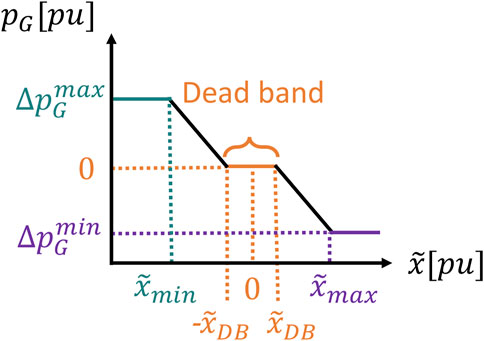
FIGURE 1. Frequency droop, the main mechanism for primary frequency control.

In MGs and ACPSs with high penetration of CIGs, where inertia may be low ($M<5s$) and power generation is typically more distributed, the alternatives are the following:

• Inertial control is usually implemented in grid-forming units (Vandoorn et al., 2013) using virtual inertia emulation (D’Arco and Suul, 2013; Fang et al., 2019). In this case, the value of $M\left(t,\tilde{x}\right)$ is a parameter of the inertia emulator. The inertial control reaction time is not instantaneous and will depend heavily on the frequency measurement algorithm and filtering techniques applied (Marchgraber et al., 2020). Furthermore, it may consume part of FCRs when activated, as grid-forming units typically provide primary control (ENTSO-E, 2019). In Europe, the set of CIGs offering inertial control is called fast frequency reserves (FFRs) (ENTSO-E, 2019).

• Primary control is provided by grid-forming and grid-following units using the frequency-droop mechanism (Vandoorn et al., 2013) akin to interconnected ACPSs. However, the reaction time is a fraction of a second because the bandwidth of a CIG controller is at least one order of magnitude larger than that of traditional turbine governors and motor drives (Fang et al., 2019).

• Secondary control is provided by grid-following units (Vandoorn et al., 2013). Considering that a MG may contain a large number of small units, manual operation can become unfeasible and automatic dispatch coordinated by a central unit, such as a MG controller, may be necessary. The reaction time of secondary control is typically faster than that in traditional ACPSs, from a couple of minutes in a large system with high penetration of CIGs (ENTSO-E, 2019) to a couple of seconds in a MG (dos Santos Alonso et al., 2019; Brandao et al., 2019).

The dynamic behavior of the average system frequency after an active power imbalance is similar for high- and low-inertia ACPSs, despite their differences, and can be divided in three periods (Eto et al., 2018):

1. Arrest: It starts immediately after the imbalance occurs. If there is lack of generation $\left(u<w\right)$, the frequency will decrease until it reaches its minimum value (nadir). If there is excess of generation $\left(u>w\right)$, the frequency will increase until it reaches its maximum value (zenith). At first, most of the balancing power $P_a$ required to stabilize the system is provided by the inertial control. Then, primary controllers gradually take over $P_a$ as the absolute value of the frequency deviation $\tilde{x}$ increases. Important metrics of this period are the rate of change of frequency (RoCoF) and the total time required to reach the nadir/zenith $t_a$.

2. Rebound: It starts immediately after the nadir/zenith is reached. During this period, the primary control is fully activated and will bring the frequency to a new equilibrium condition. This settling point is below the rated value when $u<w$ and above the rated value when $u>w$. In general, the balancing power $P_a$ is provided only by the primary control. However, the inertial control may work against the frequency restoration, as the sign of the frequency derivative can be inverted. In SMs, this negative effect is counteracted by adding damper windings in the rotor (Kundur et al., 1994). The same result can be obtained in CIGs by applying adaptive virtual inertia emulation (Fang et al., 2019). One of the important metrics of this period is the settling time $t_b$, i.e., the total time required to reach the settling point.

3. Recovery: It starts after the settling point is reached and secondary control is activated. Primary control does not have the capacity to restore the frequency to its rated value after an imbalance. Hence, the system frequency remains at the settling point until the secondary control is activated. In traditional high-inertia systems, the frequency is often restored to its rated value slowly due to practical limitations and to avoid counteraction of inertial control. However, when secondary control is fast, the rebound period can be considerably shortened and even eliminated [i.e., $t_a=t_b$ and $\tilde{x}\left(t_a\right)=\tilde{x}\left(t_b\right)$]. In the recovery period, the primary control is still active, but the secondary control gradually takes over the balancing power $P_a$, until the balance $u\left(t\right)=w\left(t\right)$ is restored. One of the important metrics of this period is the recovery time $t_c$, i.e., the total time required to reestablish the rated frequency.

Figure 2 illustrates the three control actions and the three periods following a perturbation caused by lack of generation. Even though the three periods following an active power imbalance are similar for both high- and low-inertia ACPSs, their energy management strategies for frequency control may differ considerably.

FIGURE 2

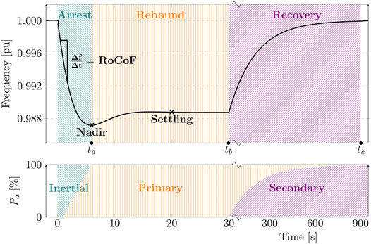
FIGURE 2. Three periods of frequency variation (arrest, rebound, and recovery) and control actions (inertial, primary, and secondary) following a perturbation caused by lack of generation.

During the arrest period, a high-inertia system relies on the rotating masses of SMs as their main energy buffer. In other words, the kinetic energy is drained from or stored into the rotor of SMs limiting the RoCoF and bounding the nadir or zenith. This energy exchange happens “automatically” without any dedicated power or control equipment because the rotor of an SM is electromagnetically coupled to its stator and, hence, the ACPS. For low-inertia systems, on the contrary, the energy buffer formed by rotating masses may not be large enough to guarantee the stable operation after a large power imbalance. In such cases, CIGs must participate as FFRs and support the system by either supplying or absorbing energy during the arrest period. The dc-link capacitor of CIGs could be considered an obvious candidate for storing the additional FFR energy. However, for power systems applications in the MW range, the required capacitance or voltage values become so high such that this solution becomes unfeasible with current technology. Therefore, an additional ESS must be sized specifically for this purpose (Milano et al., 2018).

As mentioned earlier, primary reserves are responsible for bringing the frequency from its extreme values to an acceptable settling point during the rebound phase. In traditional high-inertia systems, some generators are selected to operate with spare up and down power capacity and form FCRs. Commonly, those are dispatchable and fast-acting generating units, such as those in gas and hydropower plants, and have a large energy buffer in the form of chemical or potential energy. However, low-inertia systems may not have the necessary power or energy reserves for primary frequency control. This is because CIGs are typically connected to renewable energy sources operating in maximum power point tracking. Those have no available power up capacity and have limited down capacity. Moreover, as is the case with FFRs, the dc-link capacitor of CIGs is not designed to store the energy amount required by FCRs. In summary, an ESS must be sized to provide the energy and power capacity demanded by FCRs in low-inertia systems.

The main goal of this paper is, thus, establishing a procedure for sizing an ESS’s power and energy capacities according to its expected use (inertial control or FFRs, primary control or FCRs, or both) based on parameters that are 1) typically defined by system operators, industry standards, or network codes, 2) independent of the energy storage technology, and 3) robust to system nonlinearities. It is worth mentioning, though, that sizing the ESS for secondary control or FRRs is outside the scope of this paper. In addition, the procedure presented in the following sections assumes that a thorough stability analysis was carried out beforehand in the ACPS where the ESS will perform frequency control. This stability analysis must include measurement and actuation time delays, nonlinearities and, as a result, select or at least restrict the possible values of M and D. This type of assessment is typically a task of the transmission system operator in large and regulated ACPSs. However, this responsibility might be debatable in smaller and unregulated systems such as MGs. A detailed discussion about this topic is outside the scope of this paper, but it is worth highlighting that if ${\epsilon }_{\max }<M/D$, where ${\epsilon }_{\max }$ is the maximum time delay of all active power sources in an ACPS, then this system can be frequency stable in the presence of time delays. For details and proofs, refer to appendix B of Alves et al. (2020) and Dörfler and Bullo (2012). However, this single criterion does not guarantee global stability of the ACPS, and other aspects such as voltage, load-angle, and phase-locked loop stability must be carefully investigated.

Additional information about frequency control in high-inertia ACPSs is discussed by Kundur et al. (1994); Machowski et al. (2008); and Sauer et al. (2017). The main characteristics and challenges of low-inertia systems are reviewed by Vandoorn et al. (2013); Eto et al. (2018); Milano et al. (2018); Fang et al. (2019); dos Santos Alonso et al. (2019); and Brandao et al. (2020).

Lastly, tertiary control and generator rescheduling are further alternatives to frequency control. They are long-term, slow-response strategies based on communication infrastructure and/or electricity markets that are outside the scope of this paper. A throughout description of the European approach to these strategies is given by EU Commission Regulation (2015), while the North American approach is summarized by Eto et al. (2018).

2.2 Sizing of the Converter-Interfaced ESS Elements

This section includes the proposed procedure to size the energy capacity of the ES device and the rated power of an ES converter providing inertial or primary frequency control. Based on this initial estimation and selected references from the literature, it describes a methodology to dimension the remaining ESS power unit components.

Figure 3 presents an overview of the main elements of a converter-interfaced ESS, namely, the power and control units. In general terms, the power unit can be further subdivided into the ES device and its converter, the dc link, and the grid converter and its LC filter.

FIGURE 3

FIGURE 3. Elements of a converter-interfaced energy storage system.

2.2.1 The ES Device and Its Converter

This section proposes a method to calculate the ES converter rated power $P_{es}\left[\text{W}\right]$ and the ES device storage capacity $E_{es}\left[\text{J}\right]$ according to the type of frequency control being provided. These variables are chosen as the starting point of the sizing procedure because they are the key drivers of the ESS equipment cost (Akhil et al., 2015).

The calculation of $P_{es}\text{and}{E}_{es}$ starts by categorizing the terms of Eq. 3 in three sub-components according to the type of frequency control required to keep the power balance in the ACPS, as in the following equation, where $p_{iner}$, $p_{pri}$, and $p_{\sec }$ are, respectively, the amount of power in pu required for inertial, primary, and secondary control:

$\underset{p_{iner}}{\underbrace{\left(\tilde{x}+1\right)M\left(t,\tilde{x}\right)\dot{\tilde{x}}}}=\underset{-p_{\sec }}{\underbrace{u\left(t,\tilde{x}\right)-w\left(t,\tilde{x}\right)}}-\underset{p_{pri}}{\underbrace{\left(\tilde{x}+1\right)D\left(t,\tilde{x}\right)\tilde{x}}}.(5)$

Using this framework, algebraic expressions of $P_{es}$ and $E_{es}$ can be obtained with the following assumptions:

1. Constant inertia and damping during the interval 0 ≤ t < t_c:$M\left(t,\tilde{x}\right)\text{and}D\left(t,\tilde{x}\right)$ are constant throughout the power imbalance.

2. Primary control linearly takes over the inertial control during the interval $\mathbf{0}\le \mathit{t}<{\mathit{t}}_{\mathit{a}}$: During the arrest period, the primary control linearly takes over the balancing power from the inertial control and the contributions of the secondary control are minimal compared to the overall balancing power required. Possible time delays of controllers are ignored for the energy calculations. In addition, the RoCoF upper bound during this period can be approximated by ${\dot{\tilde{x}}}_{0a}=\tilde{x}\left(t_a\right)/t_a$.

3. The frequency nadir and zenith are bounded: The frequency nadir and zenith are enforced by either a proper combination of inertia, damping, and primary control delays or the actuation of extreme control actions such as automatic generation curtailment or load shedding (EU Commission Regulation, 2017; Eto et al., 2018).

In this case, the normalized angular speed error $\tilde{x}\left(t_a\right)$ is upper and lower bounded by ${\tilde{x}}_{tr}^{\max }$ and ${\tilde{x}}_{tr}^{\min }$, respectively. In other words, if $u<w$, then the frequency nadir is greater than ${\tilde{x}}_{tr}^{\min }$. Conversely, if $u>w$, then the frequency zenith is lower than ${\tilde{x}}_{tr}^{\max }$. Hence, if the transient frequency limit is defined as $r_{tr}=\max \left({\tilde{x}}_{tr}^{\max },{\tilde{x}}_{tr}^{\min }\right)$, then $\parallel \tilde{x}\left(t_a\right)\parallel \le r_{tr}$.

4. Only primary control is active during the interval${\mathit{t}}_{\mathit{a}}\le \mathit{t}<{\mathit{t}}_{\mathit{b}}$: During the rebound period, only the primary control is active and the contributions of the inertial control and secondary control are minimal compared to the overall balancing power required. Moreover, the RoCoF lower bound during this period can be approximated by ${\dot{\tilde{x}}}_{ab}=(\tilde{x}\left(t_b\right)-\tilde{x}\left(t_a)\right)/(t_b-t_a)$.

5. The settling point is bounded: After a power imbalance, the primary control is capable of driving the angular frequency back from the frequency zenith or nadir to within an acceptable steady-state frequency deviation $r_{ss}$. The normalized angular speed error at the settling point $\tilde{x}\left(t_b\right)$ is upper and lower bounded by ${\tilde{x}}_{ss}^{\max }$ and ${\tilde{x}}_{ss}^{\min }$, respectively. In other words, if $u<w$, then $\tilde{x}\left(t_b\right)>{\tilde{x}}_{ss}^{\min }$. Conversely, if $u>w$, then $\tilde{x}\left(t_b\right)<{\tilde{x}}_{ss}^{\max }$. Hence, if the steady-state frequency limit is defined as $r_{ss}=\max \left({\tilde{x}}_{ss}^{\max },{\tilde{x}}_{ss}^{\min }\right)$, then $\parallel \tilde{x}\left(t_b\right)\parallel \le r_{ss}$.

6. Secondary control linearly takes over during the interval ${\mathit{t}}_{\mathit{b}}\le \mathit{t}<{\mathit{t}}_{\mathit{c}}$: During the recovery period, the secondary control linearly takes over the balancing power from the primary control and the contributions of the inertial control are minimal. In addition, the RoCoF lower bound during this period can be approximated by ${\dot{x}}_{bc}=(x\left(t_c\right)-x\left(t_b)\right)/(t_c-t_b)$.

Using assumption 2, $P_{es}$ can be defined as the maximum between the components $p_{iner}$ and $p_{pri}$ in Eq. 5, as presented in Eq. 6. Using assumption 3, the bounds for $p_{iner}$ are given by Eq. 7. However, obtaining a bound to $p_{pri}$ requires an involved mathematical analysis, which is described by Alves et al. (2020), and Eq. 8 presents only the main result of this analysis:

$P_{es}=S_b\max \left(p_{es}^{iner},p_{es}^{pri}\right),(6)$

$P_{es}^{iner}=S_b\Vert \left(\tilde{x}+1\right)M\dot{\tilde{x}}\Vert \le S_b\left(1+r_{tr}\right)M\Vert \dot{\tilde{x}}\Vert ,(7)$

$P_{es}^{pri}\le S_{b}D{r}_{ss}\left(1-r_{tr}\right).(8)$

The energy required by the inertial control $E_{iner}$ and the primary control $E_{pri}$ can be calculated as the time integral of their power components defined in Eq. 2, as seen in Eq. 9 and Eq. 10. To solve these integrals analytically, it is necessary to 1) remember that $\dot{\tilde{x}}=\dot{x}=dx/dt$ and 2) use assumptions 2, 4, and 6. In Eqs. 10–13, the terms $E_{pri}^{arr},E_{pri}^{reb},\text{and}{E}_{pri}^{rec}$ are, respectively, the energy required by the primary control during the arrest, rebound, and recovery periods:

$\begin{array}{cc}{E}_{iner}& =S_b{\displaystyle \underset{0}{\overset{t_a}{\int }}\left(\tilde{x}+1\right)M\dot{\tilde{x}}dt}\\ =S_b{\displaystyle \underset{\tilde{x}\left(0\right)}{\overset{\tilde{x}\left(t_a\right)}{\int }}\left(\tilde{x}+1\right)Md\tilde{x}}\\ =S_{b}M\left[\frac{{\tilde{x}}^2\left(t_a\right)}{2}+\tilde{x}\left(t_a\right)\right],\end{array}(9)$

$\begin{array}{cc}{E}_{pri}& =\underset{E_{pri}^{arr}}{\underbrace{\frac{S_b}{2}{\displaystyle \underset{0}{\overset{t_a}{\int }}\left(\tilde{x}+1\right)D\tilde{x}dt}}}+\underset{E_{pri}^{reb}}{\underbrace{S_b{\displaystyle \underset{t_a}{\overset{t_b}{\int }}\left(\tilde{x}+1\right)D\tilde{x}dt}}}+\underset{E_{pri}^{rec}}{\underbrace{\frac{S_b}{2}{\displaystyle \underset{t_b}{\overset{t_c}{\int }}\left(\tilde{x}+1\right)D\tilde{x}dt}}}\end{array},(10)$

$\begin{array}{c}{E}_{pri}^{arr}={\frac{S_{b}D}{2{\dot{\tilde{x}}}_{0a}}\left(\frac{{\tilde{x}}^3}{3}+\frac{{\tilde{x}}^2}{2}\right)|}_0^{t_a}\\ =\frac{S_{b}D}{2}\left(t_a-t_0\right)\left[\frac{{\tilde{x}}^2\left(t_a\right)}{3}+\frac{\tilde{x}\left(t_a\right)}{2}\right],\end{array}(11)$

$\begin{array}{c}{E}_{pri}^{reb}={\frac{S_{b}D}{{\dot{\tilde{x}}}_{ab}}\left(\frac{{\tilde{x}}^3}{3}+\frac{{\tilde{x}}^2}{2}\right)|}_0^{t_a}\\ =S_{b}D\left[\frac{t_b-t_a}{\tilde{x}\left(t_b\right)-\tilde{x}\left(t_a\right)}\right]\left[\frac{{\tilde{x}}^3\left(t_b\right)-{\tilde{x}}^3\left(t_a\right)}{3}+\frac{{\tilde{x}}^2\left(t_b\right)-{\tilde{x}}^2\left(t_a\right)}{2}\right],\end{array}(12)$

$\begin{array}{c}{E}_{pri}^{rec}={\frac{S_{b}D}{2{\dot{\tilde{x}}}_{bc}}\left(\frac{{\tilde{x}}^3}{3}+\frac{{\tilde{x}}^2}{2}\right)|}_{t_b}^{t_c}\\ =\frac{S_{b}D}{2}\left(t_c-t_b\right)\left[\frac{{\tilde{x}}^2\left(t_b\right)}{3}+\frac{\tilde{x}\left(t_b\right)}{2}\right].\end{array}(13)$

To define the worst-case value for $E_{es}$, the bounds defined in assumptions 3 and 5 can be applied in Eqs. 9, 11–13, leading to the following equations:

$E_{es}\ge E_{es}^{iner}+E_{es}^{pri},(14)$

$E_{es}^{iner}\le \frac{S_{b}M}{2}{r}_{tr}\left(r_{tr}+2\right),(15)$

$E_{es}^{pri}\le E_{pri}^{arr}+E_{pri}^{reb}+E_{pri}^{rec},(16)$

$E_{pri}^{arr}\le \frac{S_{b}D}{12}\left(t_a-t_0\right)\left(2r_{tr}^2+3r_{tr}\right),(17)$

$E_{pri}^{reb}\le \frac{S_{b}D}{6}\left(t_b-t_a\right)\left(\frac{2r_{tr}^3+3r_{tr}^2-2r_{ss}^3-3r_{ss}^2}{r_{tr}-r_{ss}}\right),(18)$

$E_{pri}^{rec}\le \frac{S_{b}D}{12}\left(t_c-t_b\right)\left(2r_{ss}^2+3r_{ss}\right).(19)$

In short, a bound for $P_{es}$ and the rated power of the ES converter can be obtained with Eqs. 6–8, whereas Eqs. 14–19 can be employed for bounding $E_{es}$ and calculating the rated capacity of the ES device.

Note that $r_{tr},r_{ss},t_a,t_b,\text{and}{t}_c$ are typically defined in industry standards and network codes such as IEEE (2018a), and EU Commission Regulation, 2016. Likewise, boundaries for M, $\parallel \dot{x}\parallel$, and D can be specified based on system operator requirements or power system stability and protection coordination studies. The latter can also be used to define less conservative values of $\tilde{x}\left(t_a\right)$ and $\tilde{x}\left(t_b\right)$. In doing so, Eqs. 9, 10 can be applied to calculate $E_{es}$. Not least, the use of normalized terms $M\text{and}D$ allows system operators to specify inertia and damping requirements at the system level without knowing the installed power of a specific subsystem or installation.

2.2.2 The dc Link

The main goal of this section is to define the rated capacitance $C_{dc}\left[\text{F}\right]$ of the dc link. The dc-link capacitor is a required energy source that provides balance between the ES converter and the grid converter, allowing them to be decoupled and controlled independently. Its capacitance is defined by the following equation (Malesani et al., 1995) where $U_{dc}\left[\text{V}\right]$ is the dc-link rated voltage and $\Delta U_{dc}^{\max }$ is its maximum tolerable variation $\left[\text{V}\right]$; $T_r\left[\text{s}\right]$ represents the total time delay of the $U_{dc}$ controller; and $\Delta P_{dc}^{\max }$ is the maximum power variation in the dc link $\left[\text{W}\right]$:

$C_{dc}\ge \frac{T_r\Delta P_{dc}^{\max }}{2U_{dc}\Delta U_{dc}^{\max }}.(20)$

Typically, $U_{dc}\text{and}\Delta U_{dc}^{\max }$ are parameters associated with 1) the capacitor material and technology (Sarjeant et al., 2001), 2) the voltage class of the power switch (Infineon Technologies, 2020), and 3) network codes and requirements because variations in $U_{dc}$ will influence the maximum voltage that can be delivered by the grid converter.

The value of $T_r$ will be affected by the parameters of the $U_{dc}$ controller. If the latter is modeled as a transport delay, an estimate is given by the following equation where $T_m,T_c,\text{and}{T}_a$ are the $U_{dc}$ measurement, controller, and actuator (i.e., the ES converter) delays, respectively:

$T_r=T_m+T_c+T_a.(21)$

Finally, $\Delta P_{dc}^{\max }$ can be approximated by the active power step applied immediately after the inertial or primary controllers leave their deadband zones, as seen in Eqs. 23, 24, where $x_{DB}^{iner}\text{and}{x}_{DB}^{pri}\left[\text{pu}\right]$ are the deadband bounds of the inertial and primary control, respectively:

$\Delta P_{dc}^{\max }=\max \left(P_{iner}^{DB},P_{pri}^{DB}\right),(22)$

$P_{iner}^{DB}=2S_b{\tilde{x}}_{DB}^{iner}M\dot{\tilde{x}},(23)$

$P_{pri}^{DB}=2S_{b}D{\tilde{x}}_{DB}^{pri}.(24)$

In the approximation of Eqs. 22–24, it is assumed that $\tilde{x}$ is a smooth function. However, this assumption will not hold in an ACPS where all generators and loads are interfaced by converters because $M\to 0$ in Eq. 4 and the model and analysis presented in section 2.2.1 will no longer be valid.

2.2.3 The Grid Converter and Its LC Filter

This section discusses briefly the sizing of the grid converter and recommends references for the design of the LC filter. Figure 4 shows a schematic representation of the grid converter, the dc link, and the LC filter.

FIGURE 4

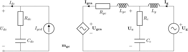
FIGURE 4. Schematic representation of the dc link and the grid converter and its LC filter.

Contractual and grid code requirements have to be taken into consideration when defining the rated apparent power of the grid converter. Among those requirements, one can mention minimum reactive power injection capacity, short-term overload, and low-voltage ride through capability (EU Commission Regulation, 2016; IEEE, 2018a). However, a relatively simple and common practice in the industry is adopted in this paper. It uses a defined or required power factor λ. The rated apparent power of the converter, $S_{gc}\left[\text{VA}\right]$, is then calculated as in the following equation:

$S_{gc}=\frac{P_{gc}}{\lambda }.(25)$

This practice generally limits the equipment size and cost. Nevertheless, it does not necessarily guarantee unsaturated operation for systems with high penetration of CIGs and MGs. In such cases, the grid converter sizing may have to consider the compensation of harmonic distortions and the definition of $S_{gc}$ will become more involved. More information about this topic can be obtained in Tenti et al. (2014).

Once $S_{gc}$ is defined, the design of the grid converter’s LC filter can start. For grid-connected converters, the LCL configuration is preferred as it limits the influence of the switching frequency harmonics in other equipment and reduces the filter size and cost (Beres et al., 2016b). Typically, the second inductance of the LCL configuration is provided by the series inductance of a step-up transformer between the ESS and the grid. The design of an LCL filter is an iterative procedure well documented in the literature, see Erickson and Maksimović, 2001; Liserre et al., 2004; Peña-Alzola et al., 2013; and Beres et al., 2016b. It can be summarized in the following steps:

1. Calculate the converter side inductance $L_{gc}$ based on the desired maximum current ripple $\Delta I_{gca}$ on the ac side of the converter, its switching frequency $f_{sw}$, and the dc-link voltage $V_{dc}$.

2. Choose the step-up transformer series inductance $L_g$ upper-bounding the total inductance $L_T=L_{gc}+L_g$ to avoid excessive voltage drop across the inductors. Note that $L_g$ is usually higher than 0.04 pu for medium-voltage transformers (ABB, 2016; Siemens, 2017). When $5\text{kHz}\le f_{sw}\le 10\text{kHz}$, it is usually possible to adopt $L_T\le 0.1\text{pu}$. On the contrary, a lower $f_{sw}$ may demand a higher $L_T$.

3. Select the filter capacitance $C_c$ upper-bounding its value to 0.05 pu (with converter rated power and voltage as the base).

4. Check if the filter resonance frequency $f_{res}$ lies between 0.2 and 0.5 times $f_{sw}$.

5. Calculate the filter damping resistance $R_c$ based on the optimal quality factor Q and maximum power losses, limiting it to $R_c^{min}=1/\left(10\text{π}{f}_{res}{C}_c\right)$ to avoid instabilities.

For that, the following equations can be used as guidelines:

$L_{gc}=\frac{U_{dc}}{24f_{sw}\Delta I_{gca}},(26)$

$L_g=0.1L_b-L_{gc},(27)$

$C_c=\frac{L_{gc}}{Z_b^2},(28)$

$f_{res}=\frac{Z_b}{2\pi L_{gc}}\sqrt{\frac{L_T}{L_g}},(29)$

$R_c=Q\sqrt{\frac{L_{gc}{L}_g}{L_T{C}_c}},(30)$

where $L_b=Z_b/{\omega }_s\text{and}{Z}_b=U_{2n}^2/S_{gc}$ are the base inductance and impedance of the grid-side converter, in which $U_{2n}$ is the rated line voltage on the low-voltage side of the step-up transformer.

It is worth emphasizing that the design of an LCL filter is iterative. Failure to comply with requirements implies restarting the whole process and changing the initial assumptions, i.e., $\Delta I_{gca},f_{sw},\text{and}{U}_{dc}$. Moreover, additional optimization objectives and constraints may require the use of high-order filters or active damping. These topics are outside the scope of this paper but can be further explored in Jalili and Bernet, 2009; Channegowda and John, 2010; Rockhill et al., 2011; Muhlethaler et al., 2013; Beres et al., 2016a; and Xu and Xie, 2018.

Finally, alternative topologies to the one presented in Figure 3 and Figure 4 are possible. Nonetheless, the principles discussed earlier in this section can also be applied to more complex solutions. For instance, ES devices using different technologies may be connected in parallel, such as ultracapacitors and batteries. The hybridization is possible because the requirements for each type of frequency control (inertial and primary) are set independently, as discussed in section 2.2.1. This also allows control strategies to operate in parallel and ES converters to share the same dc link, grid converter, and LC filter in a hybrid solution, which may help to reduce equipment costs, volume, and weight (Rocabert et al., 2019). Not least, ESSs may require more complex and robust configurations for the grid converter and consider aspects such as operating costs, efficiency, reliability, power quality, and others, as discussed by Xavier et al. (2019). However, note that these considerations will not affect the rated energy of ES devices nor the rated power of their converters, which are the variables being focused in the procedure presented in this paper.

3 Results

This section presents a case study with numerical examples demonstrating how the method and equations presented in the previous section are applied to size the main components of a hybrid, converter-interfaced ESS supplying primary and secondary frequency control to an ACPS, supported by inertial control of traditional synchronous generators.

3.1 Case Study: A Wind-Powered Offshore Platform in the North Sea

The system used as a reference is depicted in Figure 5 and represents an isolated ACPS of an offshore oil and gas platform in the North Sea.

FIGURE 5

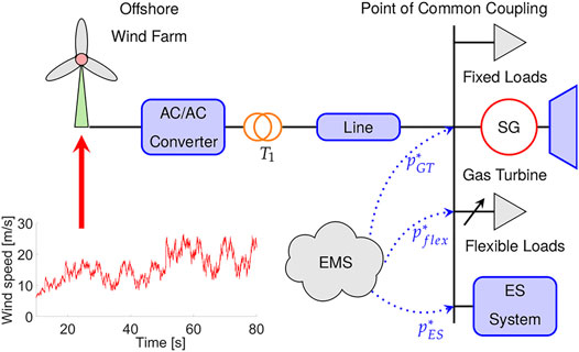
FIGURE 5. Schematic representation of the case study ACPS.

This installation operates at $60\text{Hz}$ (${\omega }_s=377{\text{rad s}}^{-1}$) and is equipped with two turbo-generators composed of an LM2500+ gas turbine from GE and an AMS 1250LG synchronous generator from ABB. Their combined active power is $70\text{MW}$, which is the value adopted for $S_b$. The normalized moment of inertia for these turbo-generators $M_{GT}$ is equal to $5.1\text{s}$. This offshore installation must comply with IEC (2019), which requires equipment to withstand frequency variations of up to 5% continuously. However, it is a goal to keep frequency variations below 2% to limit excessive overheating of electrical machines and transformers. Therefore, $r_{ss}=0.02\text{pu}$ and $r_{tr}=0.05\text{pu}$.

An initial techno-economical study of this installation (Riboldi et al., 2020) suggests that a reduction of up to 30% of its annual CO₂ emissions is possible when connecting it to a $12\text{MW}$ offshore wind farm and employing an ESS based on $4\text{MW}$ of proton exchange membrane (PEM) fuel cells and $6\text{MW}$ of PEM electrolyzers. The main goal of this hydrogen-based ESS is to stabilize the wind farm output, allowing turbo-generators to operate with optimized setpoints and, hence, attaining higher efficiencies and lower emissions. From a frequency-control perspective, the turbo-generators provide inertial control and the ESS is responsible for primary and secondary control in normal operational conditions. To limit the size of the ESS, the turbo-generators contribute with additional primary and secondary control when the ESS saturates during occasional large-frequency excursions.

Nevertheless, a high number of start–stop and load-change cycles are known to be the main drivers of PEM devices’ deterioration and performance decay (Pei et al., 2008). To avoid that, PEM fuel cells and electrolyzers are assigned to secondary control only and their load ramp rate is restricted to 0–100% in 120 s. The latter is also the value assumed for the recovery period $\left(t_c-t_b\right)$. Hence, an additional ES device must be considered to provide primary frequency control and to allow operation of the PEM fuel cells and electrolyzers in more favorable conditions.

Further on the topic primary control, it is important to mention that electric loads of this platform are divided into two groups: fixed $\left(P_{fix}=37\text{MW}\right)$ and flexible $\left(P_{flex}=7.6\text{MW}\right)$. The first group represents equipment that cannot be influenced by the energy management system (EMS) because changes in their setpoint are not possible or would affect negatively the oil and gas extraction and processing. Meanwhile, the second group represents loads whose setpoint can be temporarily raised or lowered by the EMS or primary control. An example of flexible load is the water injection system, which is responsible to maintain overall and hydrostatic reservoir pressures and force the oil toward the production wells (Devold, 2013). This type of load is flexible because reservoir pressures can vary within a certain range without considerable impacts on production. In addition, this system time constant is large (minutes) when compared to the electrical system dynamics (seconds). This concept is explored in detail by DNV-GL (2016); Sanchez et al. (2017); and Alves et al. (2019).

Hence, the water injection system can also be considered a short-term ESS that is capable of offering primary frequency control to the ACPS. When assuming that 20% of the installed flexible load can be used for primary frequency control, the following damping coefficient is obtained:

$D_{flex}=\frac{P_{flex}^{pri}}{S_b{r}_{ss}}$

$=\frac{0.2\times 7.6}{70\times 0.02}=1.09\text{pu}\text{.}$

Finally, the load demand was obtained from the platform’s supervisory control and data acquisition (SCADA) system for one representative week with a sampling period of 1 s. Figure 6 presents the histogram of this dataset, which is fit by a normal distribution when ignoring outliers below 0.6 pu. The distribution gives a load variation of $0.0428\text{pu}$ or $3\text{MW}$ in normal operational conditions with 99.9% of probability, which should be covered by primary control. Using Eq. 8,

$D_{\min }\ge \frac{p_{es}^{pri}}{r_{ss}\left(1-r_{tr}\right)}$

$\ge \frac{0.0428}{0.02\times \left(1-0.05\right)}=2.25\text{pu}\text{.}$

FIGURE 6

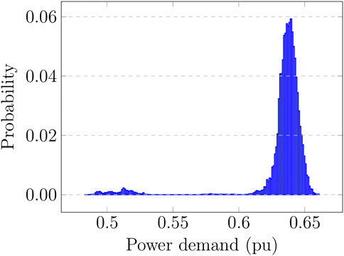
FIGURE 6. Histogram of the platform active power demand showing an average load of 0.6377 pu and a maximum variation of 0.0428 pu with 99.9% of probability when outliers below 0.6 pu are ignored.

Thus, the ES device responsible for primary control should provide the following additional damping: $D_{es}=D_{\min }-D_{flex}=1.16\text{pu}$. With these parameters, initial simulations of the case study installation for a $3\text{MW}$ load perturbation give an arrest period $\left(t_a-t_0\right)=11\text{s}$ and a rebound period $\left(t_b-t_a\right)=18\text{s}$.

Table 1 presents a summary of the installation parameters and the ESS requirements listed above.

TABLE 1

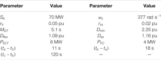
TABLE 1. Parameters of the ACPS of an offshore oil and gas platform in the Norwegian continental shelf and the requirements for its converter-interfaced ESS.

3.2 Sizing of the Energy Storage System

Applying Eqs. 8, 16 using the values from Table 1, the rated power $P_{es1}$ and energy capacity $E_{es1}$ of the ES device providing primary control can be defined as $P_{es1}=1.54\text{MW}$ and $E_{es1}=108\text{MJ}$ or $30\text{kWh}$. Note, however, that the primary control must be bidirectional, i.e., it must compensate either lack or excess of power in the system. Therefore, a 50% state of charge for the ESS in normal operation should be considered. Hence, $E_{es1}=108/0.5=219\text{MJ}$ or $60\text{kWh}$.

The most suitable ES device is chosen based on the calculated $P_{es1}$ and $E_{es1}$, on the parameters in Table 1, and on a techno-economical evaluation. The latter is not covered in this paper. It is assumed, however, that a commercial lithium-ion system such as Saft Intensium Max+ 20P (Saft, 2017) is selected. This system incorporates the ES device and converter in one assembly with two regulated dc output voltages of $771\pm 96\text{V}$ that can be connected in series or parallel and losses of about $25\text{kW}$ at rated conditions. Considering the requirements of commercial grid converters such as Siemens SINACON PV (Siemens, 2020), the ES device is assumed to have its two outputs connected in series and the following characteristics: $U_{dc}=1500\text{V}$, $\Delta U_{dc}^{\max }=150\text{V}$, $P_{losses}^{es1}=25\text{kW}$, and $T_r=2.1\text{ms}$ (one-eighth of a grid cycle).

To define $\Delta P_{dc}^{\max }$, the value $x_{DB}^{pri}=0.0025\text{pu}$ or $150\text{mHz}$ is obtained from industry standards or grid codes such as IEEE (2018a), and EU Commission Regulation, 2016. Then, $\Delta P_{dc}^{\max }=360.5\text{kW}$ is attained when applying Eqs. 22, 24. With these values defined, the dc-link capacitor is calculated using Eq. 20 and $C_{dc}\ge 1.7\text{mF}$ is retrieved.

The next step in the procedure is defining $S_{gc}$. Assuming that all ES devices share the same dc link and that the fuel cell and electrolyzer do not operate simultaneously, the active power bound will be defined by $P_{ELY}+P_{es1}+P_{losses}^{es1}=7.57\text{MW}$, where $P_{ELY}$ denotes the electrolyzer rated power. To have a buffer for the grid converter and LC filter losses, a safety margin of 2% is added to this value resulting in $P_{gc}=7.72\text{MW}$. Additionally, $\lambda =0.8$ is adopted to limit the size of the grid converter. It then follows that $S_{gc}=9.65\text{MVA}$.

The final step is calculating the components of the LC filter. For the sake of brevity, this design is not presented in this paper. The recommended procedure and references are listed in section 2.2.3. Nonetheless, the algorithm for calculating the LC filter is available for the reader in Alves (2021). The grid converter’s switching frequency is adopted as $f_{sw}=5.4\text{kHz}$ and its maximum current ripple as $\Delta I_{gca}=0.25\text{pu}$. This results in the following values for the filter components: $L_{gc}=5.61\mu \text{H}$, $L_g=6.92\mu \text{H}$, $C_c=2.5\text{mF}$, and $R_c=0.189\text{m}\Omega$. Refer to Figure 4 for the placement of each filter element. It is worth mentioning that $R_c$ yields an over-damped characteristic at the filter’s resonance frequency, which is $f_{res}=1.80\text{kHz}$ or 0.334 times $f_{sw}$.

Table 2 presents a summary of the parameters obtained above for the ESS providing primary control in the case study installation.

TABLE 2

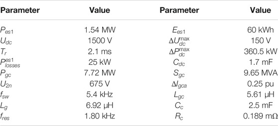
TABLE 2. Summary of the ESS parameters obtained using the proposed procedure.

3.3 Sizing Validation

To validate the calculations presented in section 3.2, a surrogate model of the case study installation was implemented in MATLAB Simulink R2018a. It has the level of details required to represent the frequency dynamics of the installation and to validate the proposed sizing of the ES device responsible for primary frequency control. It includes all main elements represented in Figure 5, namely, the turbo-generators, the fixed and flexible loads, the wind farm and its transmission line, the ESS, and the EMS. Figure 7 gives an overview of these elements in Simulink.

FIGURE 7

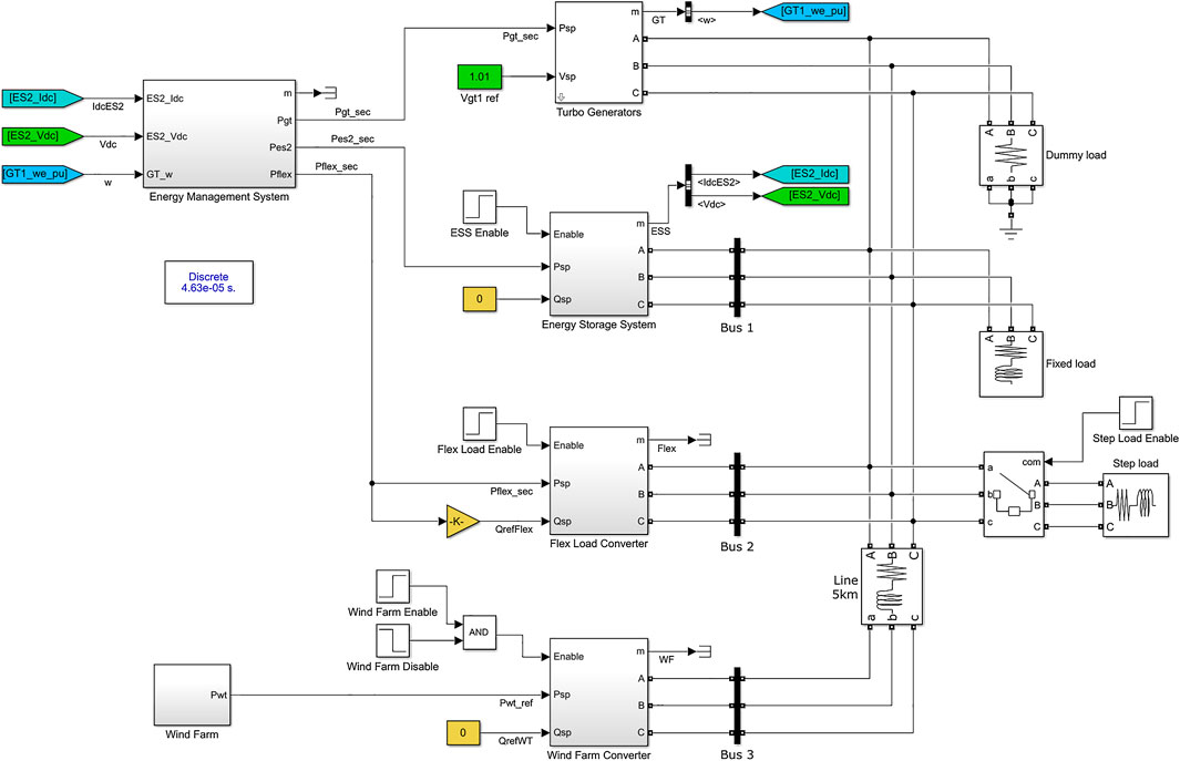
FIGURE 7. Overview of the MATLAB Simulink model used to validate the proposed sizing of the energy storage device responsible for primary control in the case study.

The model was implemented using blocks of the Simscape Electrical Specialized Power Systems toolbox complemented by an open library developed by the authors (Alves, 2020). The latter includes a generalized nonlinear droop controller that is presented in Figure 8. This block is used as the main primary frequency controller in the turbo-generators, ESSs, and flexible load subsystems with their parameters as presented in Table 3. Moreover, the secondary control is implemented in the EMS subsystem using a nonlinear integral controller from the open library with anti-windup and hold functionalities. To minimize CO₂ emissions, the EMS gives priority for changes in the ESS setpoint when the secondary control is active. The re-dispatch of turbo-generators happens only when the limits of fuel cells or electrolyzers are reached, and those may be considered a supplementary FRR.

FIGURE 8

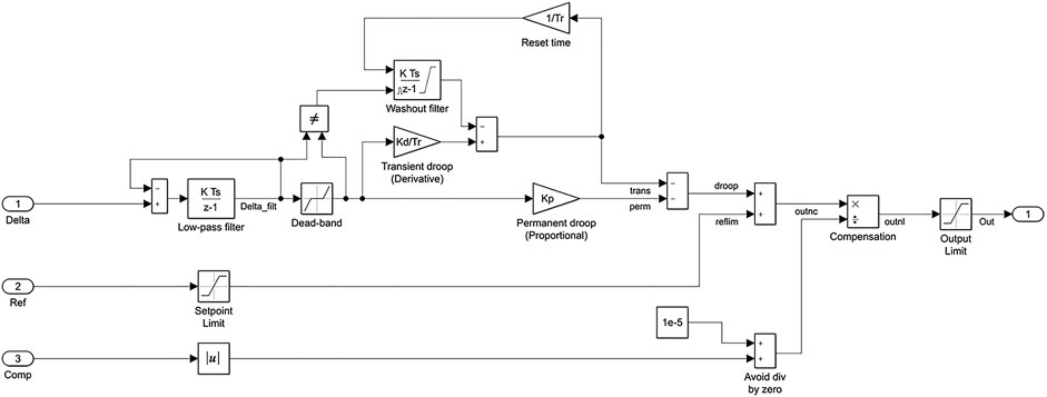
FIGURE 8. Generalized nonlinear droop controller with deadband, permanent droop (proportional gain), transient droop (derivative gain), output compensation, setpoint, and output limitation.

TABLE 3

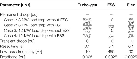
TABLE 3. Parameters of the primary controllers used during the validation.

It should be emphasized that it is not the goal of this model to validate the design of the grid converter, its controllers, or its LC filter nor to evaluate harmonics or possible power quality problems. Moreover, the validation of the fuel cell and electrolyzer stack size and their required $H_2$ storage is presented by Riboldi et al. (2021). For the sake of brevity, the validation model is not described further in this section. However, the interested reader can inspect it and find all necessary details, parameters, and simulation files to reproduce the results presented below in Alves (2021).

To create the power imbalance required for checking the ESS sizing, a load of $3\text{MW}$ (step load) is connected to the system at $t_0=2\text{s}$. As presented earlier in section 3.1, this is the expected maximum load variation under normal operational conditions with 99.9% of probability. Figure 9 shows the results of two simulations of the case study behavior during a load increase of $3\text{MW}$: Case 1 does not include the ESS in the installation, while Case 2 does include it.

FIGURE 9

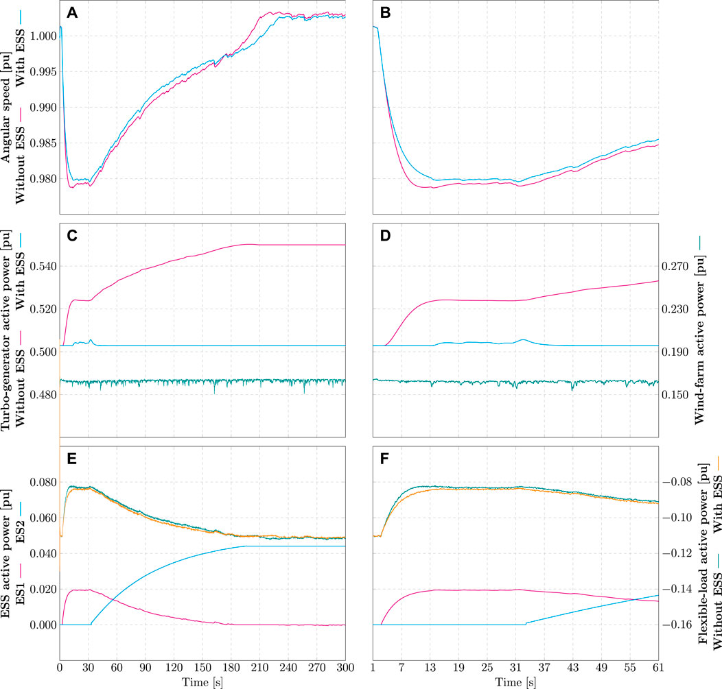
FIGURE 9. Case study behavior during a load increase of $3\text{MW}$ with and without the proposed ESS: normalized angular speed (A) during the whole transient and (B) detail of the first minute; turbo-generator and wind farm active power in pu (C) during the whole transient and (D) detail of the first minute; active power of the ES devices responsible for primary control (ES1) and secondary control (ES2) (E) during the whole transient and (F) detail of the first minute.

From a frequency-control standpoint, a closer look at Figures 9A,B reveals that the angular speed behaves similarly in both cases, i.e., with and without the ESS. The minor deviations among the cases are explained by the different deadbands and actuation delays of the turbo-generator and the ESS. Indeed, the smaller deadband and actuation delay of the converter-interfaced ESS make its performance slightly superior, achieving a higher nadir (0.9796 pu) than the turbine governor (0.9787 pu) and a smaller steady-state error (0.25 vs. 0.28%) after secondary control is deactivated. This better performance is reflected in the results seen in Figures 9E,F, which show a marginal reduction of the flexible-load active power deviation from its original setpoint while the primary control is active. Foremost, Figures 9C,D corroborate the idea proposed in section 3.2, i.e., a properly sized battery ESS would allow turbo-generators to operate at a constant setpoint when a 3 MW load variation happens suddenly while respecting the load ramp-rate limit of the PEM fuel cell, as shown in Figures 9E,F.

From a sizing perspective, the ES device responsible for primary control (battery system) delivered a peak active power of 0.0197 pu or 1.38 MW and consumed 29.4 kWh of energy. The latter was calculated by trapezoidal numerical integration of the curve ES1 in Figure 9E using a step of 100 ms. When compared to the calculated values $(1.54\text{kWh}$ and $30\text{kWh})$ from section 3.2, the proposed procedure oversized the battery system’s active power by 11.5% and its energy by 2.1%. Nonetheless, as opposed to the simulation model used for validation, the proposed procedure 1) requires knowledge of very few ACPS parameters and 2) relies only on algebraic equations, which are easy to integrate in optimization algorithms typically necessary for techno-economical evaluation of ESSs.

At this point, it is important to recap that the energy of the ES device responsible for primary control is dependent on 1) the damping $D_{es}$ provided, 2) the frequency limits $r_{ss}$ and $r_{tr}$, and 3) the duration of the arrest $\left(t_a-t_0\right)$, rebound $\left(t_b-t_a\right)$, and recovery $\left(t_c-t_b\right)$ periods, as seen in Eqs. 17–19. Thus, when defining these variables, it is critical to evaluate if the ESS must provide frequency control uninterruptedly during high-impact, low-probability events. A complete disconnection of the wind farm under full production $\left(12\text{MW}\right)$ is an example of such event for the case study presented. Figure 10 presents the results of two simulations of the case study behavior during this condition: Case 3 does not include the ESS in the installation, while Case 4 does. It is important to highlight that, for Case 3, the turbo-generator permanent droop must be increased to guarantee frequency stability and display the same dynamics of Case 4, as seen in Table 3.

FIGURE 10

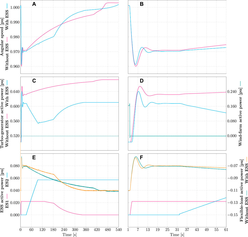
FIGURE 10. Case study behavior during the wind farm disconnection under full production ($12\text{MW}$) with and without the proposed ESS: normalized angular speed (A) during the whole transient and (B) detail of the first minute; turbo-generator and wind farm active power in pu (C) during the whole transient and (D) detail of the first minute; active power of the ES devices responsible for primary control (ES1) and secondary control (ES2) (E) during the whole transient and (F) detail of the first minute.

Figures 10A,C,E show the whole transient lasting 540 s, whereas Figures 10B,D,F zoom in its first minute. From a frequency-control point of view, Figure 10B suggests that the angular speed behaves similarly with and without the ESS during the arrest and rebound periods. However, a closer look at Figure 10A reveals that the dynamics of the recovery period in Cases 3 and 4 are distinct. This happens because the secondary controller acts differently in these two simulations.

In Case 3, the turbo-generator is the sole contributor to the FRR, and as seen in Figure 10C, its active power increases exponentially in the recovery period. As a consequence, the angular speed deviation decreases exponentially, until it reaches the deadband of the droop controller.

In Case 4, there are two sources for the FRR: the hydrogen-based ESS (preferential) and the turbo-generator (supplementary). Hence, the secondary controller ramps up the PEM fuel cell (ES2) until it reaches its rated power, as seen in Figure 10E. At the same time, the angular speed deviation decreases, and as a consequence, the droop controller reduces the turbo-generator active power, as shown in Figures 10A,C. When the ES2 limit is hit, the secondary controller starts increasing the turbo-generator active power. However, the latter is also reduced by its droop controller because the angular speed is still decreasing. These adversarial contributions continue until the deadband of the turbo-generator droop controller is reached. After that, only the secondary controller is active and the angular speed deviation decreases exponentially, until it reaches the deadband of the ES2 droop controller.

From a sizing frame of reference, the peak active power delivered by the battery system was 1.54 MW and the energy supplied was 95.6 kWh. The peak active power was limited by the nonlinear droop controller and matches the value defined in section 3.2. On the contrary, the energy obtained in the simulation is more than three times larger than the calculated value. Naturally, this happens because the parameters of the 3 and 12 MW load-increase events are disparate.

By inspection of Figure 10A, one will note that the frequency limit $r_{tr}=0.05$ was obeyed, however $r_{ss}=0.03$. Moreover, the duration of the arrest, rebound and recovery periods was $3.5\text{s},120\text{s,}\text{and}230\text{s}$. When substituting these new values in Eqs. 17–19, the energy obtained is 97 kWh, i.e., the proposed procedure oversizes the battery system’s energy by about 1.5% when compared to the simulation results. This shows that the proposed procedure can produce correct upper bounds for the ESS power and energy even when large disturbances and nonlinearities are considered.

4 Conclusions

This paper reviewed the frequency response theory in ac power systems, highlighting the different time periods (arrest, rebound, recovery) and control actions (inertial, primary, secondary) of the frequency-control problem. It also highlighted the main distinctions among traditional high-inertia systems relying on synchronous machines and low-inertia systems such as those with high penetration of converter-interfaced generation and microgrids. Grounded on these concepts and some assumptions, it derived analytical equations to rate the energy capacity and active power required by an energy storage system for providing inertial and primary control to an ac power system. The proposed equations rely on parameters typically defined by system operators, industry standards, or network codes, namely, the steady-state and transient frequency ranges, the maximum rate of change of frequency, and the desired equivalent moment of inertia and damping coefficient. Note that these parameters are independent of the technologies or topologies used in the energy storage devices and converters.

Using these results, this work also provided a step-by-step systematic procedure to initially size the remaining components of a converter-interfaced hybrid energy storage system connected to three-phase ac systems, i.e., the shared dc link and the grid converter and its LC filter. Finally, a case study of a wind-powered oil and gas platform in the North Sea was presented. It demonstrated with numerical examples how the proposed equations and the step-by-step procedure can be applied in a practical problem, where simulations in MATLAB Simulink validated the algebraic calculations and showed they slightly oversize energy storage devices. Not least, the case study demonstrated that the proposed method allows the system designer to take advantage of different energy storage technologies and set specific requirements for each storage device and converter in a hybrid system according to the type of frequency-control action being provided and requirements set by industry standards and grid codes.

Data Availability Statement

The datasets presented in this study can be found in online repositories. The names of the repository/repositories and accession number(s) can be found below: at https://zenodo.org/record/4601067 (doi 10.5281/zenodo.4384697).

Author Contributions

EA and ET conceptualized the idea. EA and DM developed the software and performed the formal analysis and investigation. EA developed the methodology, validated the results, curated the data, wrote the original draft, and produced figures and tables. ET acquired the funding, supervised and administrated the project. DM and ET reviewed and edited this paper.

Funding

This research was funded by the Research Council of Norway under the program PETROMAKS2, grant number 281986, project “Innovative Hybrid Energy System for Stable Power and Heat Supply in Offshore Oil and Gas Installation (HES-OFF),” and through the PETROSENTER scheme, under the “Research Centre for Low-Emission Technology for Petroleum Activities on the Norwegian Continental Shelf” (LowEmission), grant number 296207.

Conflict of Interest

The authors declare that the research was conducted in the absence of any commercial or financial relationships that could be construed as a potential conflict of interest.

References

ABB (2016). Technical Data for Vacuum Cast Coil Dry-Type Transformers. Zaragoza, Spain. Tech. Rep. 1LES100021-ZD.

Google Scholar

Abhyankar, S., Geng, G., Anitescu, M., Wang, X., and Dinavahi, V. (2017). Solution Techniques for Transient Stability‐constrained Optimal Power Flow - Part I. IET Generation, Transm. Distribution 11, 3177–3185. doi:10.1049/iet-gtd.2017.0345

CrossRef Full Text | Google Scholar

Aghamohammadi, M. R., and Abdolahinia, H. (2014). A New Approach for Optimal Sizing of Battery Energy Storage System for Primary Frequency Control of Islanded Microgrid. Int. J. Electr. Power Energ. Syst. 54, 325–333. doi:10.1016/j.ijepes.2013.07.005

CrossRef Full Text | Google Scholar

Ahmadi, H., and Ghasemi, H. (2014). Security-Constrained Unit Commitment With Linearized System Frequency Limit Constraints. IEEE Trans. Power Syst. 29, 1536–1545. doi:10.1109/TPWRS.2014.2297997

CrossRef Full Text | Google Scholar

Akhil, A. A., Huff, G., Currier, A. B., Kaun, B. C., Rastler, D. M., Chen, S. B., et al. (2015). DOE/EPRI Electricity Storage Handbook in Collaboration with NRECA. Sandia National Laboratories, Tech. Rep. SAND2015-1002.

CrossRef Full Text | Google Scholar

Al-Jaafreh, M. A., and Mokryani, G. (2019). Planning and Operation of LV Distribution Networks: A Comprehensive Review. IET Energ. Syst. Integ. 1, 133–146. doi:10.1049/iet-esi.2019.0013

CrossRef Full Text | Google Scholar

Alves, E. F., Bergna, G., Brandao, D. I., and Tedeschi, E. (2020). Sufficient Conditions for Robust Frequency Stability of AC Power Systems. IEEE Trans. Power Syst. 1, 1. doi:10.1109/TPWRS.2020.3039832

CrossRef Full Text | Google Scholar

Alves, E. F. (2021). Efantnu/hybrid-ess-design: Review 1 Release. version v1.1Zenodo. doi:10.5281/zenodo.4601067

CrossRef Full Text

Alves, E. F. (2020). Efantnu/pwrsys-matlab. Zenodo. doi:10.5281/zenodo.4384758

CrossRef Full Text | Google Scholar

Alves, E., Sanchez, S., Brandao, D., and Tedeschi, E. (2019). Smart Load Management with Energy Storage for Power Quality Enhancement in Wind-Powered Oil and Gas Applications. Energies 12, 2985. doi:10.3390/en12152985

CrossRef Full Text | Google Scholar

Beres, R. N., Wang, X., Blaabjerg, F., Liserre, M., and Bak, C. L. (2016a). Optimal Design of High-Order Passive-Damped Filters for Grid-Connected Applications. IEEE Trans. Power Electron. 31, 2083–2098. doi:10.1109/TPEL.2015.2441299

CrossRef Full Text | Google Scholar

Beres, R. N., Wang, X., Liserre, M., Blaabjerg, F., and Bak, C. L. (2016b). A Review of Passive Power Filters for Three-Phase Grid-Connected Voltage-Source Converters. IEEE J. Emerg. Sel. Top. Power Electron. 4, 54–69. doi:10.1109/JESTPE.2015.2507203

CrossRef Full Text | Google Scholar

Bijaieh, M. M., Weaver, W. W., and Robinett, R. D. (2020a). Energy Storage Power and Energy Sizing and Specification Using HSSPFC. Electronics 9, 638. doi:10.3390/electronics9040638

CrossRef Full Text | Google Scholar

Bijaieh, M. M., Weaver, W. W., and Robinett, R. D. (2020b). Energy Storage Requirements for Inverter-Based Microgrids Under Droop Control in D-Q Coordinates. IEEE Trans. Energ. Convers. 35, 611–620. doi:10.1109/TEC.2019.2959189

CrossRef Full Text | Google Scholar

Brandao, D. I., Araujo, L. S., Alonso, A. M. S., dos Reis, G. L., Liberado, E. V., and Marafao, F. P. (2020). Coordinated Control of Distributed Three- and Single-Phase Inverters Connected to Three-Phase Three-Wire Microgrids. IEEE J. Emerg. Sel. Top. Power Electron. 8, 3861, 3877. doi:10.1109/JESTPE.2019.2931122

CrossRef Full Text | Google Scholar

Brandao, D. I., Ferreira, W. M., Alonso, A. M. S., Tedeschi, E., and Marafao, F. P. (2020). Optimal Multiobjective Control of Low-Voltage AC Microgrids: Power Flow Regulation and Compensation of Reactive Power and Unbalance. IEEE Trans. Smart Grid 11, 1239–1252. doi:10.1109/TSG.2019.2933790

CrossRef Full Text | Google Scholar

Caliskan, S. Y., and Tabuada, P. (2015). “Uses and Abuses of the Swing Equation Model,” in 2015 54th IEEE Conference on Decision and Control (CDC), Osaka, Japan, December 15–December 18, 2015, 6662–6667. doi:10.1109/CDC.2015.7403268

CrossRef Full Text | Google Scholar

Chang, G. W., Chuang, C.-S., Lu, T.-K., and Wu, C.-C. (2013). Frequency-regulating Reserve Constrained Unit Commitment for an Isolated Power System. IEEE Trans. Power Syst. 28, 578–586. doi:10.1109/TPWRS.2012.2208126

CrossRef Full Text | Google Scholar

Channegowda, P., and John, V. (2010). Filter Optimization for Grid Interactive Voltage Source Inverters. IEEE Trans. Ind. Electron. 57, 4106–4114. doi:10.1109/TIE.2010.2042421

CrossRef Full Text | Google Scholar

Concordia, C. (1951). Synchronous Machines, Theory and Performance. (New York, NY: Wiley).

D’Arco, S., and Suul, J. A. (2013). Virtual Synchronous Machines — Classification of Implementations and Analysis of Equivalence to Droop Controllers for Microgrids. PowerTech (Grenoble, France: IEEE), 1–7. doi:10.1109/PTC.2013.6652456

CrossRef Full Text | Google Scholar

Delille, G., Francois, B., and Malarange, G. (2012). Dynamic Frequency Control Support by Energy Storage to Reduce the Impact of Wind and Solar Generation on Isolated Power System's Inertia. IEEE Trans. Sustain. Energ. 3, 931–939. doi:10.1109/TSTE.2012.2205025

CrossRef Full Text | Google Scholar

Devold, H. (2013). Oil and Gas Production Handbook: An Introduction to Oil and Gas Production, Transport, Refining and Petrochemical Industry (Oslo: ABB). (Accessed July 17, 2020).

Google Scholar

DNV-GL (2016). Joint Industry Project: Wind-Powered Water Injection. Høvik, Norway, Tech. rep., DNV-GL.

Google Scholar

Doherty, R. E., and Nickle, C. A. (1927). Synchronous Machines-III Torque-Angle Characteristics Under Transient Conditions. Trans. Am. Inst. Electr. Eng. XLVI, 1–18. doi:10.1109/T-AIEE.1927.5061336

CrossRef Full Text | Google Scholar

Dörfler, F., and Bullo, F. (2012). Synchronization and Transient Stability in Power Networks and Nonuniform Kuramoto Oscillators. SIAM J. Control. Optim. 50, 1616–1642. doi:10.1137/110851584

CrossRef Full Text | Google Scholar

dos Santos Alonso, A. M., Carlos Afonso, L., Brandao, D. I., Tedeschi, E., and Marafao, F. P. (2019). “Considerations on Communication Infrastructures for Cooperative Operation of Smart Inverters,” in 2019 IEEE 15th Brazilian Power Electronics Conference and 5th IEEE Southern Power Electronics Conference COBEP/SPEC). (Santos, Brazil: IEEE). doi:10.1109/COBEP/SPEC44138.2019.9065382

CrossRef Full Text | Google Scholar

Duckwitz, D. (2019). Power System Inertia: Derivation of Requirements and Comparison of Inertia Emulation Methods for Converter-Based Power Plants. PhD thesis. Kassel (Germany): University of Kassel.

Google Scholar

Egido, I., Sigrist, L., Lobato, E., Rouco, L., and Barrado, A. (2015). An Ultra-capacitor for Frequency Stability Enhancement in Small-Isolated Power Systems: Models, Simulation and Field Tests. Appl. Energ. 137, 670–676. doi:10.1016/j.apenergy.2014.08.041

CrossRef Full Text | Google Scholar

Entso-E, (2019). Fast Frequency Reserve – Solution to the Nordic Inertia Challenge. Tech. rep., Entso-e.

Google Scholar

Erickson, R. W., and Maksimović, D. (2001). Fundamentals of Power Electronics. 2 edn. Springer. doi:10.1007/b100747

CrossRef Full Text

Eto, J. H., Undrill, J., Roberts, C., Mackin, P., and Ellis, J. (2018). Frequency Control Requirements for Reliable Interconnection Frequency Response. Lawrence Berkeley National Laboratory, Tech. Rep. LBNL-2001103.

Google Scholar

EU Commission Regulation (2015). Guideline on Capacity Allocation and Congestion managementTech. Rep. Brussels, Belgium: European Union. EU 2015/1222 Online. (Accessed July 17, 2020).

EU Commission Regulation (2017). Guideline on Electricity Transmission System OperationTech. Rep. Brussels, Belgium: European Union. EU 2017/1485Online. (Accessed July 17, 2020).

EU Commission Regulation (2016). Network Code on Requirements for Grid Connection of Generators. EU 2016/631. Tech. Rep. Brussels, Belgium: European Union. Online. (Accessed July 17, 2020).

Fang, J., Li, H., Tang, Y., and Blaabjerg, F. (2019). On the Inertia of Future More-Electronics Power Systems. IEEE J. Emerg. Sel. Top. Power Electron. 7, 2130–2146. doi:10.1109/JESTPE.2018.2877766

CrossRef Full Text | Google Scholar

Farhadi, M., and Mohammed, O. (2016). Energy Storage Technologies for High-Power Applications. IEEE Trans. Ind. Applicat. 52, 1953–1961. doi:10.1109/TIA.2015.2511096

CrossRef Full Text | Google Scholar

Fu, Q., Hamidi, A., Nasiri, A., Bhavaraju, V., Krstic, S. B., and Theisen, P. (2013). The Role of Energy Storage in a Microgrid Concept: Examining the Opportunities and Promise of Microgrids. IEEE Electrific. Mag. 1, 21–29. doi:10.1109/MELE.2013.2294736

CrossRef Full Text | Google Scholar

Gallo, A. B., Simões-Moreira, J. R., Costa, H. K. M., Santos, M. M., and Moutinho dos Santos, E. (2016). Energy Storage in the Energy Transition Context: A Technology Review. Renew. Sustain. Energ. Rev. 65, 800–822. doi:10.1016/j.rser.2016.07.028

CrossRef Full Text | Google Scholar

Gamarra, C., and Guerrero, J. M. (2015). Computational Optimization Techniques Applied to Microgrids Planning: A Review. Renew. Sustain. Energ. Rev. 48, 413–424. doi:10.1016/j.rser.2015.04.025

CrossRef Full Text | Google Scholar

Geng, G., Abhyankar, S., Wang, X., and Dinavahi, V. (2017). Solution Techniques for Transient Stability‐constrained Optimal Power Flow - Part II. IET Generation, Transm. Distribution 11, 3186–3193. doi:10.1049/iet-gtd.2017.0346

CrossRef Full Text | Google Scholar

Grainger, J. J., and Stevenson, W. D. (1994). Power System Analysis. New York, NY: McGraw-Hill Series in Electrical and Computer Engineering McGraw-Hill.

Hemmati, R., and Saboori, H. (2016). Emergence of Hybrid Energy Storage Systems in Renewable Energy and Transport Applications - A Review. Renew. Sustain. Energ. Rev. 65, 11–23. doi:10.1016/j.rser.2016.06.029

CrossRef Full Text | Google Scholar

IEC (2019). IEC 61892:2019 Mobile and Fixed Offshore Units - Electrical Installations. Geneva, Switzerland: IEC.

IEEE (2018a). IEEE 1547-2018 - IEEE Standard for Interconnection and Interoperability of Distributed Energy Resources with Associated Electric Power Systems Interfaces. New York, NY: IEEE.

IEEE (2018b). IEEE 2030.8-2018 IEEE Standard for the Testing of Microgrid Controllers. New York, NY: IEEE.

Infineon Technologies (2020). Power and Sensing Selection Guide 2020. Tech. rep., Infineon Technologies Austria AG.

Jalili, K., and Bernet, S. (2009). Design of LCL Filters of Active-Front-End Two-Level Voltage-Source Converters. IEEE Trans. Ind. Electron. 56, 1674–1689. doi:10.1109/TIE.2008.2011251

CrossRef Full Text | Google Scholar

Kimbark, E. W. (1995). Power System Stability. New York, NY: IEEE Press Power Systems Engineering Series, IEEE Press.

Knap, V., Chaudhary, S. K., Stroe, D.-I., Swierczynski, M., Craciun, B.-I., and Teodorescu, R. (2016). Sizing of an Energy Storage System for Grid Inertial Response and Primary Frequency Reserve. IEEE Trans. Power Syst. 31, 3447–3456. doi:10.1109/TPWRS.2015.2503565

CrossRef Full Text | Google Scholar

Koohi-Kamali, S., Tyagi, V. V., Rahim, N. A., Panwar, N. L., and Mokhlis, H. (2013). Emergence of Energy Storage Technologies as the Solution for Reliable Operation of Smart Power Systems: A Review. Renew. Sustain. Energ. Rev. 25, 135–165. doi:10.1016/j.rser.2013.03.056

CrossRef Full Text | Google Scholar

Kundur, P., Balu, N. J., and Lauby, M. G. (1994). Power System Stability and Control. The EPRI Power System Engineering. New York, NY: McGraw-Hill.

Google Scholar

Liserre, M., Blaabjerg, F., and Dell’Aquila, A. (2004). Step-by-step Design Procedure for a Grid-Connected Three-phase PWM Voltage Source Converter. Int. J. Electron. 91, 445–460. doi:10.1080/00207210412331306186

CrossRef Full Text | Google Scholar

Machowski, J., Bialek, J. W., and Bumby, J. R. (2008). Power System Dynamics: Stability and Control. 2nd edn. Chichester, U.K: Wiley.

Malesani, L., Rossetto, L., Tenti, P., and Tomasin, P. (1995). AC/DC/AC PWM Converter with Reduced Energy Storage in the DC Link. IEEE Trans. Ind. Applicat. 31, 287–292. doi:10.1109/28.370275

CrossRef Full Text | Google Scholar

Marchgraber, J., Alács, C., Guo, Y., Gawlik, W., Anta, A., Stimmer, A., et al. (2020). Comparison of Control Strategies to Realize Synthetic Inertia in Converters. Energies 13, 3491. doi:10.3390/en13133491

CrossRef Full Text | Google Scholar

Milano, F., Dorfler, F., Hug, G., Hill, D. J., and Verbic, G. (2018). “Foundations and Challenges of Low-Inertia Systems,” in 2018 Power Systems Computation Conference (PSCC). Dublin: IEEE, 1–25. doi:10.23919/PSCC.2018.8450880

CrossRef Full Text | Google Scholar

Muhlethaler, J., Schweizer, M., Blattmann, R., Kolar, J. W., and Ecklebe, A. (2013). Optimal Design of LCL Harmonic Filters for Three-Phase PFC Rectifiers. IEEE Trans. Power Electron. 28, 3114–3125. doi:10.1109/TPEL.2012.2225641

CrossRef Full Text | Google Scholar

Nguyen, N., Almasabi, S., Bera, A., and Mitra, J. (2019). Optimal Power Flow Incorporating Frequency Security Constraint. IEEE Trans. Ind. Appl. 55, 6508–6516. doi:10.1109/TIA.2019.2938918

CrossRef Full Text | Google Scholar

Pei, P., Chang, Q., and Tang, T. (2008). A Quick Evaluating Method for Automotive Fuel Cell Lifetime. Int. J. Hydrogen Energ. 33, 3829–3836. doi:10.1016/j.ijhydene.2008.04.048

CrossRef Full Text | Google Scholar

Peña-Alzola, R., Liserre, M., Blaabjerg, F., Sebastián, R., Dannehl, J., and Fuchs, F. W. (2013). Analysis of the Passive Damping Losses in LCL-Filter-Based Grid Converters. IEEE Trans. Power Electron. 28, 2642–2646. doi:10.1109/TPEL.2012.2222931

CrossRef Full Text | Google Scholar

Riboldi, L., Alves, E. F., Pilarczyk, M., Tedeschi, E., and Nord, L. O. (2020). “Innovative Hybrid Energy System for Stable Power and Heat Supply in Offshore Oil & Gas Installation (HES-OFF): System Design and Grid Stability,” in 30th European Symposium on Computer Aided Process Engineering (ESCAPE30). Milano, Italy: Elsevier.

Google Scholar

Riboldi, L., Alves, E. F., Pilarczyk, M., Tedeschi, E., and Nord, L. O. (2021). Optimal Design of a Hybrid Energy System for the Supply of Clean and Stable Energy to Offshore Installations. Front. Energ. Res. doi:10.3389/fenrg.2020.607284

CrossRef Full Text | Google Scholar

Rocabert, J., Capo-Misut, R., Munoz-Aguilar, R. S., Candela, J. I., and Rodriguez, P. (2019). Control of Energy Storage System Integrating Electrochemical Batteries and Supercapacitors for Grid-Connected Applications. IEEE Trans. Ind. Applicat. 55, 1853–1862. doi:10.1109/TIA.2018.2873534

CrossRef Full Text | Google Scholar

Rockhill, A. A., Liserre, M., Teodorescu, R., and Rodriguez, P. (2011). Grid-Filter Design for a Multimegawatt Medium-Voltage Voltage-Source Inverter. IEEE Trans. Ind. Electron. 58, 1205–1217. doi:10.1109/TIE.2010.2087293

CrossRef Full Text | Google Scholar

Saft, (2017). Intensium Max+ 20P Product Datasheet. Tech. rep., Saft.

Google Scholar

Sanchez, S., Tedeschi, E., Silva, J., Jafar, M., and Marichalar, A. (2017). Smart Load Management of Water Injection Systems in Offshore Oil and Gas Platforms Integrating Wind Power. IET Renew. Power Generation 11, 1153–1162. doi:10.1049/iet-rpg.2016.0989

CrossRef Full Text | Google Scholar

Sandelic, M., Stroe, D.-I., and Iov, F. (2018). Battery Storage-Based Frequency Containment Reserves in Large Wind Penetrated Scenarios: A Practical Approach to Sizing. Energies 11, 3065. doi:10.3390/en11113065

CrossRef Full Text | Google Scholar

Sarjeant, W., Clelland, I., and Price, R. (2001). Capacitive Components for Power Electronics. Proc. IEEE 89, 846–855. doi:10.1109/5.931475

CrossRef Full Text | Google Scholar

Sauer, P. W., Pai, M. A., and Chow, J. H. (2017). Power System Dynamics and Stability: With Synchrophasor Measurement and Power System Toolbox. 2nd Edn. Hoboken, NJ: Wiley.

Siemens, (2020). SINACON PV Photovoltaic Central Inverter Technical Data. Erlangen, Germany, Tech. Rep. SIDS-B10020-00-7600, Siemens AG.

Google Scholar

Siemens, (2017). The GEAFOL Neo: The Optimum Foundation for Power Distribution. Erlangen, Germany, Tech. Rep. EMTR-B10021-00-7600, Siemens AG.

Google Scholar

Strbac, G., Hatziargyriou, N., Lopes, J. P., Moreira, C., Dimeas, A., and Papadaskalopoulos, D. (2015). Microgrids: Enhancing the Resilience of the European Megagrid. IEEE Power Energ. Mag. 13, 35–43. doi:10.1109/MPE.2015.2397336

CrossRef Full Text | Google Scholar

Tavora, C. J., and Smith, O. J. M. (1972). Characterization of Equilibrium and Stability in Power Systems. IEEE Trans. Power Apparatus Syst. Pas- 91, 1127–1130. doi:10.1109/TPAS.1972.293468

CrossRef Full Text | Google Scholar

Tenti, P., Costabeber, A., Mattavelli, P., Marafao, F. P., and Paredes, H. K. M. (2014). Load Characterization and Revenue Metering Under Non-Sinusoidal and Asymmetrical Operation. IEEE Trans. Instrum. Meas. 63, 422–431. doi:10.1109/TIM.2013.2280480

CrossRef Full Text | Google Scholar

Vandoorn, T. L., Vasquez, J. C., De Kooning, J., Guerrero, J. M., and Vandevelde, L. (2013). Microgrids: Hierarchical Control and an Overview of the Control and Reserve Management Strategies. IEEE Ind. Electron. Mag. 7, 42–55. doi:10.1109/MIE.2013.2279306

CrossRef Full Text | Google Scholar

Wen, Y., Li, W., Huang, G., and Liu, X. (2016). Frequency Dynamics Constrained Unit Commitment With Battery Energy Storage. IEEE Trans. Power Syst. 31, 5115–5125. doi:10.1109/TPWRS.2016.2521882

CrossRef Full Text | Google Scholar

Xavier, L. S., Amorim, W. C. S., Cupertino, A. F., Mendes, V. F., do Boaventura, W. C., and Pereira, H. A. (2019). Power Converters for Battery Energy Storage Systems Connected to Medium Voltage Systems: A Comprehensive Review. BMC Energy 1, 7. doi:10.1186/s42500-019-0006-5

CrossRef Full Text | Google Scholar

Xu, J., and Xie, S. (2018). LCL-resonance Damping Strategies for Grid-Connected Inverters with LCL Filters: A Comprehensive Review. J. Mod. Power Syst. Clean. Energ. 6, 292–305. doi:10.1007/s40565-017-0319-7

CrossRef Full Text | Google Scholar

Nomenclature

ACPS ac power system

CIG converter-interfaced generator

EMS energy management system

ES energy storage

ESS energy storage system

FCRs frequency containment reserves

FFRs fast frequency reserves

FRRs frequency restoration reserves

FSM frequency sensitivity mode

MG microgrid

RoCoF rate of change of frequency

PEM proton exchange membrane

SCADA supervisory control and data acquisition

SM synchronous machine