A Two-Stage Dispatching Method for Wind-Hydropower-Pumped Storage Integrated Power Systems

With the fossil energy crisis and environmental pollution, wind energy and other renewable energy have been booming. However, the strong intermittence and volatility of wind power make difficult of its integration into grid. To solve this problem, this study proposes a complementary power generation model of wind-hydropower-pumped storage systems, which uses hydropower and pumped storage to adjust the fluctuation of wind power. How to consider the uncertainty and unpredictability of wind power output and make more reliable hydropower generation plan and pumped storage generation plan is the key problem to be solved in the grid with the high proportion of renewable energy. The martingale model of forecast evolution is used to describe the uncertainty evolution of wind power in different regions. According to the flexible load in the region, the flexibility index is used to quantify flexibility, and the transaction price is set to be proportional to flexibility. The two-stage framework of day-ahead and real-time dispatching model is then developed. In the day-ahead stage, different regions trade with each other. If the power after trading is imbalanced, it will be supplemented by hydropower and the grid to meet the power demand. In the real-time stage, the pumped storage is added to quickly balance the deviation of wind power and load between the real-time and day-ahead stages. Finally, considering the positive effect of hydropower on wind power consumption in the grid, a benefit allocation method based on improved Shapley value method is proposed. Test cases are simulated to verify the rationality of the proposed dispatching model and the benefit allocation method. After the cooperation of hydropower and pumped storage, the average revenue growth is 3.02%. The improved benefit allocation scheme makes more benefit of hydropower and pumped storage and promotes the cooperation of multi-participants.

Introduction

With the transformation of the global energy structure, the installed capacity of renewable energy has been increasing steadily (Bird et al., 2016). According to forecasts by the International Energy Agency, the proportion of renewable energy in global electricity consumption should be up to 30% by 2023 (International Energy Agency, 2018). Grid-connected power generation of large-scale renewable energy, which is represented by solar and wind energy, has become an unstoppable development trend of new power systems. However, the uncertainty of renewable energy would cause the curtailment of power and the fluctuation of output. The utilization of renewable energy is impeded severely, and the dispatching of the power system is also influenced greatly. Hydropower, which has a strong regulation capability, is usually used as an adjustable power supply to ensure a stable and smooth output (Zhang et al., 2019). The pumped storage has the advantage of flexible schedulability and the ability of fast start-up and shut-down (Javed et al., 2020). Therefore, the complementary power generation system, which coordinates wind power with hydropower and pumped storage, can efficiently solve problems caused by the uncertainty of renewable energy and is important for the stability and economy of wind-hydropower-pumped storage (WHPS) systems.

In recent years, the modeling and optimization of complementary power generation system between renewable energy and other power have been conducted in many studies, mainly including hydro-wind (Denault et al., 2009; Lopes and Borges, 2014; Bayon et al., 2016; Shayesteh et al., 2016), hydro-solar-wind (Schmidt et al., 2016; Liu et al., 2019; Zhang et al., 2019), hydro-wind-thermal (Zhou et al., 2016; Zhang et al., 2017), solar-wind- pumped storage (Jakub et al., 2018; Xu et al., 2019), and wind-solar-storage (Lee and Wang, 2008; Lasemi and Arabkoohsar, 2020). The main idea is to combine renewable energy with hydropower and other flexible power and then improve the power grid’s ability to consume renewable energy and schedulability. Gebretsadik et al. (Gebretsadik et al., 2016) proposed an operation model of wind power and hydropower to maximize the generation of integrated wind and hydropower. Li et al. (Li and Qiu, 2016) used hydropower to compensate for photovoltaic power as the great adjustable capability of hydropower. Panda et al. (Panda et al., 2017) developed a combined operation model of hydro-thermal-wind, and its optimal generation schedule is determined by a different algorithm. Biswas et al. (Biswas et al., 2018) proposed the optimization method of stochastic wind, solar, and small hydropower, considering intermittent and uncertain of renewable sources. Reddy et al. (Reddy, 2017) solved an optimal scheduling problem of the hybrid power system, concluding thermal generators, wind power, and solar power with batteries. Wang et al. (Wang et al., 2017) proposed the coordinated operation of the hydro-wind-photovoltaic system to overcome the bottleneck of new energy development.

Although these studies have researched the complementary operations of multi-power systems, the wind power uncertainties, which have made challenges of its large integration in the power system, still need to be considered thoroughly. Some researchers have investigated the uncertainty of wind power and emphasize the influence of wind power uncertainties on dispatching. Shahriari et al. (Shahriari et al., 2020) used the probabilistic method for wind power forecasting, which could quantify the uncertainty associated with wind forecast rather than deterministic forecast; probabilistic forecast is critical for users and dispatchers to make informed decisions. Zhang et al. (Zhang et al., 2014) verified that wind power forecast involves inherent uncertainty because of chaotic climatic and weather conditions, and probabilistic forecast is critical in the uncertainty atmospheric environment. Turk et al. (Turk et al., 2020) introduced that high level of uncertainty and fluctuation of renewable energy sources exist and proposed the scenario generation algorithm with corresponding probabilities to improve the utilization of wind energy. Li et al. (Li et al., 2020) discussed and classified the scenario generation method to address the uncertainties of energy systems with integrated wind power. In the above studies, the ways to describe the uncertainty of renewable energy can be classified as probabilistic forecasting, scenario generation, and uncertainty description by conditional value at risk. These methods usually assume that the error is fixed in a certain period. However, the weather system is dynamic and unstable, and wind power output is closely related to wind speed, temperature, wind direction, and other meteorological factors. The dynamic uncertainty of wind power should be updated as the forecast lead-time gradually increases. In current studies, only a few studies have considered the evolution of renewable energy uncertainty, which would have a certain impact on the dispatching results of multi-power systems.

In addition to the above problems, the complementary operation of wind power and hydropower can complement the output fluctuation caused by the uncertainty and improve the utilization of wind power. However, it may affect the hydropower adversely because of some reasons (e.g., the release of ecological water to the downstream river channel) and influence its ability of peaking capability. When wind power output is large, the hydropower generation would be reduced, and the possibility of hydroelectric spillage would be increased to ensure minimum ecological water delivery. The revenue of hydropower may be reduced through complementary operations. Therefore, how to make a reasonable allocation of benefit and stimulate the enthusiasm of hydropower to cooperation with wind power remains to be studied. Based on the basic principles of income distribution, the Shapley theory was developed by Shapley in 1953 (Liggett and Rumelt, 2009). In terms of benefit allocation between different units, some studies have been conducted. Shen et al. (Shen et al., 2018) allocated the appropriate benefit of multiple-reservoir cascaded hydropower plants by the game-theoretic Shapley method. Tan et al. (Tan et al., 2013) used the Shapley method to study the benefit allocation of wind power and thermal power; the result showed that the method realized the equitable allocation among the units fully. Wu et al. (Wu et al., 2019) proposed a benefit allocation mechanism based on Shapley value and nucleolus solution, and the corresponding effectiveness and applicability were proven. Kristiansen et al. (Kristiansen et al., 2018) used the Shapley value to access the benefits of fast-ramping gas turbine and hydropower, and the insights for energy policy designs could be gained through this way. However, the traditional Shapley method has some disadvantages. All stakeholders are assumed to have equal risks and status. Thus, the traditional Shapley value method should be improved according to the specific projects.

This study proposes a two-stage coordinated operation model of the WHPS system. Each of the three regions consists of wind power and flexible load. They trade with one another first. If there exist power shortage, the power can be provided from the hydropower or the grid; If there exist excess power, they can be sold to the grid in the day-ahead stage. In the real-time stage, considering the deviation of wind power and load between the real-time and day-ahead stages, the pumped storage, which can start and stop quickly, is used to balance the deviation. The main contributions of this study include the following:

Considering the constant updates and the evolution of wind power forecasting, the martingale model of forecast evolution (MMFE) is used to describe the evolution process of wind power forecasting uncertainty, and the synthetic ensemble forecasts are generated.

In the day-ahead stage, after regions trade with one another, if no balance is achieved, power is purchased or sold from hydropower or grid. In the real-time stage, the forecasting deviation of wind power and load between real-time and day-ahead is balanced by the pumped storage. The output fluctuation to the grid can be mitigated.

Considering the risk and cost factors of different members, the improved Shapley value method, which has a practical significance, is proposed to consider the characteristics of different participants fully and ensure their reasonable benefit allocation.

The rest of this paper is organized as follows. Martingale Model of Wind Power Forecasting. Coordinated Operation Model of the WHPS System. Benefit Allocation Model by the Improved Shapley Value Method. Solution Method. Case Study and compares the Benefit Allocation of the Traditional Shapley Method and the Improved Shapley Method. Finally, Conclusion concludes the paper.

Martingale Model of Wind Power Forecasting Evaluation

The description of the forecast uncertainty of wind speed over time is vital for power grid dispatching. However, only a few methods can illustrate the evolution process of forecasting uncertainty. In this section, the MMFE is established for the evolution of the uncertainty of wind power forecasting over time. The MMFE was first proposed to simulate the uncertainty of supply chain demand forecasting (Heath and Jackson, 1994). This method is simple and effective; the mean value and covariance are used and are not invariant as traditional scene generation methods; the time-variation of wind power forecasting uncertainty is considered (Zhao et al., 2011).

Uncertainty of Wind Power Forecast

As time progresses, the forecasting information of wind power will be updated constantly. $H$ is defined as the forecasting horizon, and $P_{w,t}^{\text{wind}}$ is defined as the forecasting value for wind power at time $t$, which is made at time $w$$\left(t=ws+0,ws+1,\cdots ,ws+H\right)$. $P_t^{\text{wind}}$ identifies the actual value of wind power, and $e_{w,t}$ denotes the forecasting error, which can be interpreted by Eq. 1.

$e_{w,t}=P_{w,t}^{wind}-P_t^{wind}(1)$

The sequence of forecasting value with the forecasting horizon ranges from 0 to $H$, and the corresponding error made at time $w$ can be expressed as follows:

$P_{w,-}^{\text{wind}}=\left[P_{w,w}^{\text{wind}},P_{w,w+1}^{\text{wind}},\cdots ,P_{w,w+H}^{\text{wind}}\right](2)$

$e_{w,-}=\left[e_{w,w}\text{,}{e}_{w,w+1},\cdots ,e_{w,w+H}\right](3)$

Similarly, the wind power value of time $t$ can be forecasted in the previous period. The sequence and the corresponding error are expressed as follows:

$P_{-,t}^{\text{wind}}=\left[P_{t-H,t}^{\text{wind}},P_{t-H+1,t}^{\text{wind}},\cdots ,P_{t,t}^{\text{wind}}\right](4)$

$e_{-,t}=\left[e_{t-H,t}\text{,}{e}_{t-H+1,t},\cdots ,e_{t,t}\right](5)$

The improvement of forecasting value is defined as the difference of forecasting error between two adjacent time $w-1$ and $w$ is expressed as follows:

$u_{w,t}=e_{w,t}-e_{w-1,t}(6)$

Assuming that the current wind power forecasting value is accurate ($e_{t,t}=0$), based on Eqs. 4–6, the following equation can be obtained.

$\{\begin{array}{l}{e}_{t-1,t}=e_{t,t}-u_{t,t}=-u_{t,t}\\ e_{t-2,t}=e_{t-1,t}-u_{t-1,t}=-u_{t,t}-u_{t-1,t}\\ \cdots \\ e_{t-H,t}=-{\displaystyle \sum _{i=1}^H{u}_{t-H+i,t}}\end{array}(7)$

Based on Eqs. 1Eqs. 7 the forecasting value $P_{t,t}^{\text{wind}}$ can be expressed by the actual value and the improvement value, which is shown as follows:

$\{\begin{array}{l}{P}_{t,t}^{\text{wind}}=P_t^{\text{wind}}\\ P_{t-1,t}^{\text{wind}}=P_t^{\text{wind}}-u_{t,t}\\ P_{t-2,t}^{\text{wind}}=P_t^{\text{wind}}-u_{t,t}-u_{t-1,t}\\ \cdots \\ P_{t-H+1,t}^{\text{wind}}=P_t^{\text{wind}}-{\displaystyle \sum _{i=1}^{H-2}{u}_{t-i+1,t}}\\ P_{t-HL,t}^{\text{wind}}=P_t^{\text{wind}}-{\displaystyle \sum _{i=1}^{HL-1}{u}_{t-i,t}}\end{array}(8)$

The above formula can be transformed into the following equation:

$\{\begin{array}{l}{P}_{t,t}^{\text{wind}}=P_{t-1,t}^{\text{wind}}+u_{t,t}\\ P_{t-1,t}^{\text{wind}}=P_{t-2,t}^{\text{wind}}+u_{t-1,t}\\ \cdots \\ P_{t-H+1,t}^{\text{wind}}=P_{t-H,t}^{\text{wind}}+u_{t-H+1,t}\end{array}(9)$

Eq. 9 shows that, as time progresses from $t-H$ to $t$, the forecasting value $P_{w,t}^{\text{wind}}$ will update constantly as $u_{w,t}$ updates.

The MMFE

In the MMFE, the forecasting improvement value $u_{w,w+i-1}$$\left(i=\mathrm{1,2},\cdots ,H\right)$ can be expressed as follows:

$U_{w,-}=\left[u_{w,w},u_{w,w+1},\cdots ,u_{w,w+H-1}\right](10)$

In the MMFE model, $U_{w,-}$ describes the uncertainty of wind power with four kinds of assumptions (Heath and Jackson, 1994): 1) The mean value of $u_{w,w+i-1}$ is zero (i.e., unbiased assumption), 2) $u_{w,w+i-1}$ obeys normal distribution (i.e., Gaussian distribution), 3) $u_{w1,w+i-1}$ is independent with $u_{w2,w+i-1}$ (i.e., temporal independence assumption), and 4) the distribution of $u_{w,w+i-1}$ does not change over time (i.e., stationarity assumption). On the basis of the above assumptions, the MMFE model can be expressed using the variance-covariance (VCV) matrix as follows:

$VCV=\left[\begin{array}{l}{\mathrm{var}}_1{\text{ cov}}_{\mathrm{1,2}}\cdots {\text{ cov}}_{1,H}\\ {\text{cov}}_{\mathrm{2,1}}{\text{ var}}_2\cdots {\text{ cov}}_{2,H}\\ ⋮⋮\ddots ⋮\\ {\text{cov}}_{H,1}{\text{ cov}}_{H,2}\cdots {\text{var}}_H\end{array}\right](11)$

Given that $VCV$ is a positive semi-definite matrix, it can be decomposed into the product of matrix $V$ and its transpose by Cholesky decomposition (i.e., $VCV=V\times V^T$). The vector $U_{w,-}$ can be expressed through a mathematical transformation as follows:

$\left[u_1{u}_2\cdots u_H\right]=\left[x_1{x}_2\cdots x_H\right]V^T(12)$

where $x_i\left(i=\mathrm{1,2},\cdots ,H\right)$ is the independent random variable with the same standard normal distribution, $VCV$ is the variance-covariance matrix of vector $U_{w,-}$, ${\mathrm{var}}_i$ is the variance of $u_{w,w+i-1}$, and ${\text{cov}}_{i,j}$ is the covariance between $u_{w,w+i-1}$ and $u_{w,w+j-1}$. After obtaining $x_1{x}_2\cdots x_H$ and $U_{w,-}$, combined with Eq. 9, the wind power forecasting value can be generated synthetically.

Coordinated Operation Model of the Wind-Hydropower-Pumped Storage System

The multi-power system investigated in this study is composed of hydropower, wind power, and pumped storage. The relationship among different members is shown in Figure 1. The hydropower output is a wide range. The pumped storage has flexible schedulability. The hydropower and pumped storage can ensure the smooth and stable output curve when wind power is strongly uncertain. Wind power and flexible loads form a region, when wind power output is greater than the load, the net power in the region is positive, this region can be considered as power supply. When wind power output is less than the load, the net power generation is negative, this region can be considered as the load. Three regions trade with one another firstly. If no balance is achieved after trading, power is purchased or sold from hydropower and grid in the day-ahead stage. In the real-time stage, the deviation of wind power and the load between the real-time and day-ahead stages are considered. The pumped storage, which can start and stop quickly, is used to balance the deviation. The power shortage in the region can be supplemented effectively by the above method, and the grid’s ability to wind power consumption would be improved.

FIGURE 1

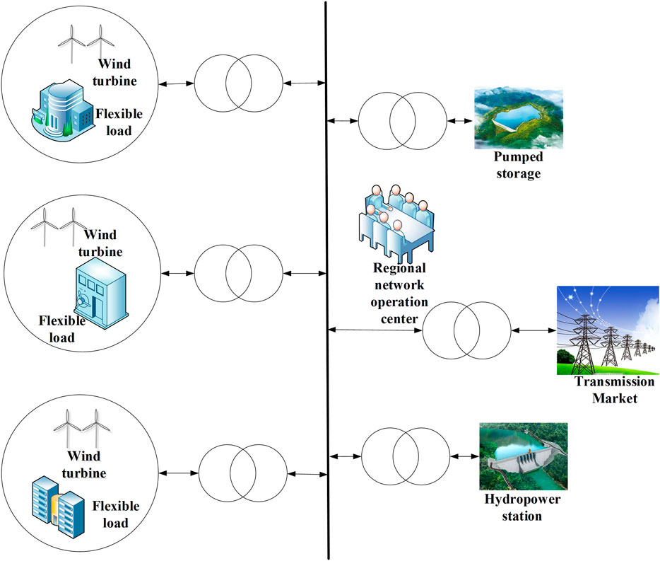
FIGURE 1. Relationship among different members.

Modeling of the Wind-Hydropower-Pumped Storage Complementary Power Generation System

(1) Modeling of the Hydropower Station

The hydropower station has flexible regulation performance. The output can be expressed as the product of a constant, the generation efficiency of hydropower station, the net head, and the average power generation flow of the corresponding period. The output model can be expressed as follows:

$P_{\text{hyd,}i,t}=0.00981{\eta }_i{H}_{i,t}{Q}_{i,t}^{\text{H}}(13)$

where $P_{\text{hyd,}i,t}$ is the output of hydropower station $i$ at time $t$, $Q_{i,t}^H$ is the average power generation flow, $H_{i,t}$ is the net head, and ${\eta }_i$ is the power generation efficiency of the hydropower station $i$.

(2) Transformational relationship of hydropower station

The storage capacity of cascade hydropower stations should consider interval water. The interval water of the reservoir contains the natural water, generation flow, and the abandoned water of the upstream reservoir. The relationship equation is as follows:

$V_{i,t}=V_{i,t\mathrm{-}1}+3600\left(Q_{i,t}^S\mathrm{-}{Q}_{i,t}^H\mathrm{-}{Q}_{i,t}^d\right)(14)$

$V_{i,0}=V_{i,\text{T}}+\text{Δ}{V}_i(15)$

$Q_{i,t}^S=I_{i,t}+Q_{i-1,t}^H+Q_{i-1,t}^d(16)$

where $V_{i,t}$ is the storage capacity of the reservoir $i$ at time $t$, $V_{i,t\mathrm{-}1}$ is the storage capacity of the reservoir $i$ at time $t\mathrm{-}1$, $Q_{i,t}^S$ is the interval water of the reservoir at time $t$, $I_{i,t}$ is the volume of natural water, $V_{i,0}$ is the initial water level, $V_{i,\text{T}}$ is the final water level of the reservoir $i$, $\text{Δ}{V}_i$ is the variance of storage capacity, $Q_{i,t}^d$ is the volume of abandoned water, $Q_{i,t}^H$ is the volume of generation flow, and $Q_{i\mathrm{-}1,t}^d$ and $Q_{i\mathrm{-}1,t}^H$ are the volume of abandoned water and the generation flow of the upstream reservoir, respectively.

(3) Inequality constraint of hydropower station

The output, storage capacity, and flow of the hydropower station have upper and lower limit constraints:

$P_{\text{hyd},i}^{\text{min}}\le P_{\text{hyd},i,t}\le P_{\text{hyd},i}^{\text{max}}(17)$

$V_{i,\text{min}}\le V_{i,t}\le V_{i,\text{max}}(18)$

$Q_{i,\text{min}}^H\le Q_{i,\text{t}}^H\le Q_{i,\text{max}}^H(19)$

where $P_{\text{hyd},i}^{\text{min}}$ and $P_{\text{hyd},i}^{\text{max}}$ are the minimum and maximum output of hydropower station $i$, respectively; $V_{i,\text{min}}$ and $V_{i,\text{max}}$ are the minimum and maximum storage capacity, respectively, and $Q_{i,\text{min}}^H$ and $Q_{i,\text{max}}^H$ are the minimum and maximum flow, respectively.

(4) Volume conversion constraints of pumped storage station

The pumped storage station can utilize the characteristics of power generation and pumping to realize the transfer of power generation and rapid regulation of the total output. The pumped storage station contains the upstream and downstream reservoirs, and their constraints are the same. Generally, only the upstream reservoir is constrained as follows:

$V_{\text{pm},k,t}=V_{\text{pm},k,t-1}+{\eta }_{\text{pm},k}\text{Δ}t{P}_{\text{pm},k,t}-{\eta }_{\text{gn},k}\text{Δ}t{P}_{\text{gn},k,t}(20)$

where $V_{\text{pm},k,t}$ is the volume of pumped storage $i$ at time $t$; $V_{\text{pm},k,t\mathrm{-}1}$ is the volume of pumped storage $i$ at time $t-1$; ${\eta }_{\text{pm},k}$ and ${\eta }_{\text{gn},k}$ are the power/water conversion coefficient at pumping and generation conditions, respectively; $P_{\text{pm},k,t}$ and $P_{\text{gn},k,t}$ are the pumping and generation power of the pumped storage station, respectively.

(5) Volume constraints of pumped storage station

The volume of the pumped storage station should be within a certain range, and it is the same at the beginning and end of the day. It can be expressed as follows:

$V_{\text{pm},k}^{\text{min}}\le V_{\text{pm},k,t}\le V_{\text{pm},k}^{\text{max}}(21)$

$V_{\text{pm},k,0}=V_{\text{pm},k,\text{T}}(22)$

where $V_{\text{pm},k}^{\text{max}}$ and $V_{\text{pm},k}^{\text{min}}$ are the maximum and minimum volume of the pumped storage, respectively, and $V_{\text{pm,}k\text{,0}}$ and $V_{\text{pm},k,\text{T}}$ are the initial and final volume of the pumped storage during the scheduling period, respectively.

(6) Working condition constraints of the pumped storage station

The working condition constraints of the pumped storage are generation and pumping, and the two kinds of condition never exist at the same time. The detailed constraint is as follows:

$y_{\text{pm},k,t}+y_{\text{gn},k,t}\le 1y_{\text{pm},k,t},y_{\text{gn},k,t}\in \left\{\mathrm{0,1}\right\}(23)$

When $y_{\text{pm},k,t}=1$, the pumped storage station is in the pumping condition. When $y_{\text{gn},k,t}=1$, the pumped storage station is in the generation condition. When $y_{\text{pm},k,t}=y_{\text{gn},k,t}=0$, the pumped storage station is idle.

(7) Output constraints of pumped storage station

$\{\begin{array}{l}{y}_{\text{pm},k,t}{P}_{\text{pm},k}^{\text{min}}\le P_{\text{pm},k,t}\le y_{\text{pm},k,t}{P}_{\text{pm},k}^{\text{max}}\\ y_{\text{gn},k,t}{P}_{\text{gn},k}^{\text{min}}\le P_{\text{gn},k,t}\le y_{\text{gn},k,t}{P}_{\text{gn},k}^{\text{max}}\end{array}(24)$

where $P_{\text{pm,}k}^{\text{min}}$ and $P_{\text{pm,}k}^{\text{max}}$ are the minimum and maximum pumping power of pumped storage k, respectively, and $P_{\text{gn,}k}^{\text{min}}$ and $P_{\text{gn,}k}^{\text{max}}$ are the minimum and maximum generation power, respectively.

(8) Pumping/generation condition conversion downtime constraints

Generally, the continuous start and stop of pumped storage station is not carried out under pumping or generation conditions. For economic reasons, the pumped storage should be shut down for at least 1 h. The corresponding constraint is as follows:

$\{\begin{array}{l}{y}_{\text{pm},k,t}+y_{\text{gn},k,t+1}\le \begin{array}{cc}1& t=\mathrm{1,2},\cdots ,T-1\end{array}\\ y_{\text{pm},k,t+1}+y_{\text{gn},k,t}\le \begin{array}{cc}1& t=\mathrm{1,2},\cdots ,T-1\end{array}\end{array}(25)$

(9) Constraints of load in a region

$P_{i,t}^{\text{da,load,min}}\le P_{i,t}^{\text{da,load}}\le P_{i,t}^{\text{da,load,max}}(26)$

where $P_{i,t}^{da,load,\min }$ is the minimum value of load and $P_{i,t}^{da,load,\max }$ is the maximum value of the load.

(10) Constraints of tie line’s volatility ratio

$\frac{\left|P_{\text{grid,}t}-P_{\text{grid,}t-1}\right|}{P_{\text{grid,}t}^{\max }}\le K_{\text{grid}}^{\max }(27)$

$P_{\text{grid,}t}=P_{\text{hyd},t}+P_t(28)$

$P_t={\displaystyle \sum _{i=1}^I\left(P_{i,t}^{\text{wind}}-P_{i,t}^{\text{load}}\right)}(29)$

where $P_t^{ch}=P_{grid,t}^{da}+P_{mar,t}^{re}$, $P_{grid,t}$ is the trading power with the grid at time $t$, $P_{\text{grid,}t\mathrm{-}1}$ is the trading power with the grid at time $t-1$, $P_{\text{grid,}t}^{\max }$ is the maximum value of trading power with the grid, $K_{\text{grid}}^{\max }$ is the tie line’s volatility ratio, $P_{\text{hyd},t}$ is the generation power of hydropower, and $P_t$ is the net power of regions. The smaller the value of $K_{\text{grid}}^{\max }$, the better the complementary effect of the complementary power generation system.

Objective Function

(1) Day-ahead stage

The coordinate operation of WHPS system uses multi-source complementary characteristics fully. Each kind of power supply is encouraged to play its role, and the goal of the economy and the stability of system operation are realized. In the day-ahead stage, considering the large peak regulation capacity and strong regulation capacity of the cascade hydropower stations, its joint operation with wind power is an effective way to solve large-scale wind power consumption. The power generation in the region meets the load in the region. If the power generation and load are unbalanced, different regions would trade with each other. After that, if power is redundant, the power is sold to the grid. If a power shortage is still experienced, the hydropower and grid can provide power. The specific objective of the economic operation is to minimize the generation cost in the dispatching period. The corresponding day-ahead objective function is as follows:

$\max R_{V,t}={\chi }_{1,t}{C}_{1,t}{P}_{1,t}+{\chi }_{2,t}{C}_{2,t}{P}_{2,t}+{\chi }_{3,t}{C}_{3,t}{P}_{3,t}+{\chi }_{grid,t}{C}_{grid,t}{P}_{grid,t}{+\text{C}}_{hyd,t}{P}_{hyd,t}{+\text{C}}_{hyd,t}^d(30)$

where ${\chi }_{i,t}$ is the state variable of region $i$. When redundant power exists in this region, the state variable is 1. When it is short of power, the state variable is 0. $C_{i,t}$ is the bidding price of region $i$, $P_{i,t}$ is the purchase or sale power of region $i$, ${\chi }_{grid,t}$ is the state variable of grid, $C_{grid,t}$ is the power price in the day-ahead stage, $P_{grid,t}$ is the purchase or sale of power of the grid, ${\text{C}}_{hyd,t}$ is the price of hydropower, $P_{hyd,t}$ is the output of hydropower, and $C_{hyd,t}^d$ is the cost of abandoned water. According to the understanding of its load regulation ability, each flexible load can predict the lower and upper limits of its total load in a certain period in the future, the minimum value of the load is express as $P_{i,t}^{da,load,\min }$, and the maximum value of the load is expressed as $P_{i,t}^{da,load,\max }$. The flexible load needs to report its load range $\left[P_{i,t}^{da,load,\min },P_{i,t}^{da,load,\max }\right]$ to the stage organizer. $P_{i,t}^{da,load,\max }-P_{i,t}^{da,load,\min }$ represents the fluctuation of power that the load can bear. The flexibility indicator of the load is defined as follows:

${\kappa }_{i,t}=\frac{P_{i,t}^{\max }-P_{i,t}^{\min }}{P_{i,t}^{\max }+P_{i,t}^{\min }}(31)$

The net power generation or the load of region $i$ as power supply or load is as follows:

$P_{i,t}^{\text{da}}=P_{i,t}^{\text{da,wind}}-P_{i,t}^{\text{da,load}}(32)$

where $P_{i,t}^{da,wind}$ is the wind power output of region $i$ at time $t$ and $P_{i,t}^{da,load}$ is the load of region $i$ at time $t$. If $P_{i,t}^{da,wind}>P_{i,t}^{da,load}$, region $i$ is the power supply. The bidding of each region is related to its flexibility. The higher the flexibility, the higher the bidding. The equation is $C_{i,t}=\left(1+{\kappa }_{i,t}\right){\lambda }_{i,t}$, where ${\lambda }_{i,t}$ is the basic price. If $P_{i,t}^{da,wind}<P_{i,t}^{da,load}$, region $i$ is the load. The higher the flexibility, the lower the bidding. The corresponding equation is $C_{i,t}=\left(1-{\kappa }_{i,t}\right){\lambda }_{i,t}$. To reflect the relationship between regional flexibility and the final transaction price, the final transaction price is the data after the bidding and market clearing price are processed in proportion. The transaction price further reflects the flexibility of each region.

(2) Real-time stage

In the real-time stage, the pumped-storage, which is as a flexible power, can operate jointly with multiple regions containing wind farms to smooth the deviations of wind power and load between day-ahead and real-time stages. The optimization model is to optimize the trading power of pumped storage, grid, and three regions simultaneously. The optimization strategy considers the spot price, the start-up and shutdown cost of pumped storage, and other factors. The objective shown as follows minimizes the total operation cost of the system.

$\max R^{re}={\displaystyle \sum _{t=1}^T{R}_{mar,t}^{re}}-{\displaystyle \sum _{t=1}^T{C}_{\text{pm,t}}}(33)$

where $R_{re}$ is the net revenue in the real-time stage, $R_{mar,t}^{re}$ is the revenue from selling to the grid, $C_{\text{pm,t}}$ is the cost of pumped storage.

Although the pumped storage unit starts and stops quickly, the working condition can be adjusted flexibly. However, physical loss will be caused in the process of frequent start-up and shutdown. The cost of pumped storage contains the start-up cost of generation and pumping and can be expressed as follows:

$C_{\text{pm}}={\displaystyle \sum _{t=1}^T{\displaystyle \sum _{k=1}^{n_k}\left(C_{\text{pm},k,t}+C_{\text{gn},k,t}\right)}}(34)$

where $C_{\text{pm},k,t}$ is the start-up/shut-down cost of pumping and $C_{\text{gn},k,t}$ is the start-up/shut-down cost of generation. The revenue that sold to the grid can be expressed as follows:

$R_{mar,t}^{re}={\displaystyle \sum _{t=1}^T{P}_{mar,t}^{re}{\lambda }_t^{re}}(35)$

$P_{\text{mar},t}^{\text{re}}={\displaystyle \sum _{i=1}^I\left(P_{i,t}^{\text{re}}-P_{i,t}^{\text{da}}\right)}+{\displaystyle \sum _k^K\left(P_{k,t}^{\text{gn}}-P_{k,t}^{\text{pum}}\right)}(36)$

$P_{i,t}^{\text{re}}=P_{i,t}^{\text{re,wind}}-P_{i,t}^{\text{re,load}}(37)$

where $P_{mar,t}^{re}$ is the power sold to the grid in the real-time stage, ${\lambda }_t^{re}$ is spot price at time $t$, $P_{i,t}^{da}$ is the net power in the day-ahead stage, $P_{i,t}^{re}$ is the net power in the real-time stage, $P_{k,t}^{gn}$ is the power generation of pumped storage, and $P_{k,t}^{pum}$ is the value of pumping.

Benefit Allocation Model by the Improved Shapley Value Method

Cooperative Game Theory

Game theory is mainly used to study how to choose the best decision or group decision-making when interesting relations or conflicts between multiple decision-makers are observed (Yang et al., 2020). This method focuses on how many people cooperate to maximize the benefits of the alliance and how to distribute the benefits. A single agent participating in the market is faced with uncertain risks, such as its output and market price. However, given that the cooperative game alliance is composed of multi-agents, the multi-power complementary system can reduce its risk through internal regulation. Thus, additional benefits (i.e., cooperation surplus) are obtained. How to allocate the cooperative surplus reasonably is the key factor that affects whether different agents can reach a cooperative relationship.

Regarding the alliance $N=\left\{\mathrm{1,2,3},\cdots ,n\right\}$ of $n$ members, $S$ is a subset of $N$, which represents a kind of combination. Assuming that the revenue of member $i$ after the distribution is $R_i$, $R\left(S\right)$ is the revenue of $S$, and $R\left(\left\{\text{i}\right\}\right)$ is the revenue of member $i$ without cooperation. Generally, an alliance can maintain cooperation needs to meet three conditions: 1) the individual revenue of each member is increased after cooperation, 2) the total revenue of alliance is increased after cooperation, and 3) the total benefit remains steady before and after benefit allocation.

$R_i\ge R\left(\left\{i\right\}\right)(38)$

$R\left(S\right)\ge {\displaystyle \sum _{i\in S}R\left(\left\{i\right\}\right)}(39)$

${\displaystyle {\sum }_{i=1}^n{R}_i=R\left(N\right)}(40)$

The Traditional Shapley Value Method

The Shapley value method focuses on the marginal revenue of each member and determines the benefit that should be shared by all members by calculating the expected value of the marginal contribution of each member. Assuming $n$ members in the alliance, they can be expressed as $N=\left\{\mathrm{1,2},\mathrm{...},n\right\}$, the formula for calculating the benefit allocated to member $i$ is as follows:

$v_i={\displaystyle \sum _{S\in N}\omega }\left(\left|S\right|\right)\left[v\left(S\right)-v\left(S/i\right)\right],i=\mathrm{1,2},\mathrm{...},n(41)$

$\omega \left(\left|S\right|\right)=\frac{\left(n-\left|S\right|\right)!\left(\left|S\right|\mathrm{-}1\right)!}{n!}(42)$

where $\omega \left(\left|S\right|\right)$ is the weighting factor, $v\left(S\right)$ is the revenue of set $S$, $v\left(S/i\right)$ is the revenue when member $i$ is deleted from set $S$, and $\left|S\right|$ is the number of members in set $S$.

Improved Benefit Allocation Model

The traditional Shapley value method has some shortcomings. The risks of different members in the alliance are regarded as equal, and other factors that need to be considered in the benefit distribution are simplified and ignored. In the actual cooperation alliance, the risk and cost factors of different members are different, and their willingness to participate in the alliance is also different. If all members are regarded as the same, the rationality of the final benefit allocation is affected. To make up for the shortcomings of the traditional Shapley method, in this study, the risk and cost factors are considered in the adjustment of the traditional Shapley value, and an improved benefit allocation model considering multi-factors is proposed.

Risk Factor

Risk sharing is a key problem in the process of the WHPS integrated power system. The greater the risk the participants take in the process of cooperation, the greater the expected benefits. The different risks of different members lead to the difficulty of benefit allocation in the system. Therefore, introducing the risk factor for reasonable benefit distribution is crucial.

${\phi }_i^R{\left(V_i\right)}^{\text{'}}=R\times \Delta R_i+V_i(43)$

where $R$ is the total revenue, $\Delta R_i$ is the difference between the risk taken by member $i$ and the average risk (i.e., $\Delta R_i=R_i-\frac{R}{n}$), $\Delta R_i$ is also known as the risk correction factor, $V_i$ is the allocated benefit of member $i$ by traditional Shapley method, and ${\phi }_i^R{\left(V_i\right)}^{\text{'}}$ is the benefit allocation result by the improved Shapley method with considering risk factor.

Cost Factor

The proposed cost factor focuses on the costs of all members in the actual operation process of the multi-power system. The benefit allocation of the participants is also affected by their cost. Generally, the higher the cost, the higher the expected benefits. The addition of the cost factor is beneficial to the rationality of benefit allocation. The equation is as follows:

$\chi \left(V_i\right)=C\times \Delta C_i+V_i(44)$

where $C$ is the total revenue, $\Delta C_i$ is the difference between the cost of member $i$ and the average cost (i.e., $\Delta C_i=\frac{C_i}{C}-\frac{1}{n}$), $\Delta C_i$ is also known as the cost correction factor, and $\chi \left(V_i\right)$ is the benefit allocation result by the improved Shapley method with the cost factor.

Solution Method

Based on the martingale model, the scenario of the wind power output considering the evolution uncertainty of wind power forecasting is generated. In the day-ahead stage, the power supply and load demand of each region are analyzed, and the net power of this region can be calculated. Three regions trade with each other. If the power after trading remains unbalanced, it can be adjusted by purchasing power from hydropower or selling power to a large power grid. In the real-time stage, pumped storage is used to balance the deviation of wind power and load between the real-time and day-ahead stages quickly. An improved benefit allocation method that considers the risk and cost factors of each subject on the basic of Shapley value is put forward, which can reasonably allocate the benefits generated by the cooperation of multi-regions, the hydropower, and pumped storage. Using the uncertainty analysis formula of wind power in Eqs. 9–12, the revenue of the day-ahead stage shown in Eqs. 30–32, the revenue of the real-time stage shown in Eqs. 33–37, the improved benefit allocation of multi-members shown in Eqs. 41–44. Using the above model, Lingo is used to solve the problem. The revenue of each region after trading among the three regions in the day-ahead stage is obtained. The revenue, which is from three regions and the hydropower sale to the grid after hydropower is engaged in cooperation, can be obtained. In the real-time stage, the revenue of regions and pumped storage that sell to the grid can also be obtained. The result of the benefit allocation is obtained using the improved Shapley value method. The flowchart of dispatching and benefit allocation is shown in Figure 2.

FIGURE 2

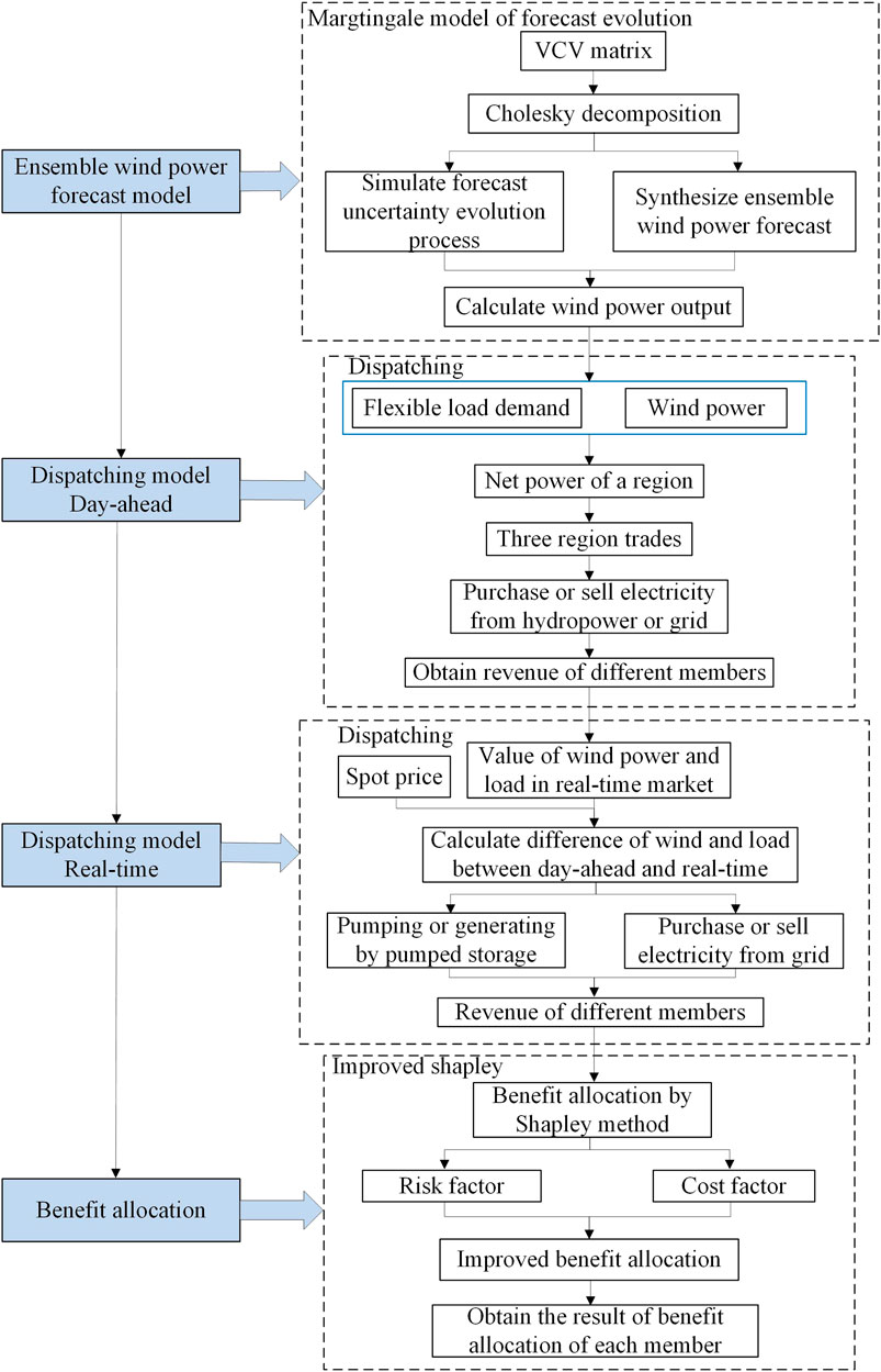
FIGURE 2. Flowchart of dispatching and benefit allocation.

The specific steps are as follows:

Using the MMFE to synthesize the ensemble wind power forecasting, this method keeps the statistical moments of the generated wind power sequence, such as mean and variance, and considers the evolution of wind power uncertainty over time.

The optimal dispatching of the day-ahead stage is carried out. First, according to its flexible load demand and wind power generation, the net power of each region is calculated. Next, if excess or shortage of power is experienced in the three regions, they will trade with each other. Then, if the three regions are balanced in power, the real-time stage is entered; if not, a shortage of power is experienced in the three regions, which can be supplemented by hydropower or by purchasing power from the grid. When the three regions have excess power, they can sell to the grid.

In the real-time stage, the deviation of wind power and load between the real-time and day-ahead stages is calculated. Considering the deviation and the spot price, the power generation and pumping of pumped storage are optimized, and the trading power between multi-regions and the grid is obtained. Through this method, the deviation is made up, the economy is improved, and the risk is reduced.

Considering that part of the interests of hydropower and pumped storage have been reduced to stabilize the fluctuation of wind power, the benefit generated after cooperation should be distributed among regions, hydropower, and pumped storage. Given that the traditional Shapley method does not consider the difference of different members, the risk and cost factors are introduced to obtain the improved benefit distribution scheme.

Case Study

Basic Data

To show the change of wind forecast uncertainty over time, the proposed MMFE model is used to generate the ensemble forecasts of wind power synthetically. The time scale of wind power synthetic ensemble forecasts is 24 h, and the time interval is 1 h. Figures 3–5 show the value of wind power in different regions over time in a day. As can be seen, with the increase of forecast lead time, the variance of wind power forecasting is also increased. Most of the time, the values of forecasted wind power are evenly distributed on both sides of the average value. As time progresses, the amount of data on two sides of the mean value gradually varies because of the increased uncertainty of the forecast over time. Three typical scenarios are then selected from the generated wind power for the later analysis. The first one is the value of the upper quartile, which is shown in red. The second one is the mean value, which is shown in yellow. The third one is the value of the lower quartile, which is shown in blue. Figure 6 shows the mean value and the range of flexible load in the three regions.

FIGURE 3

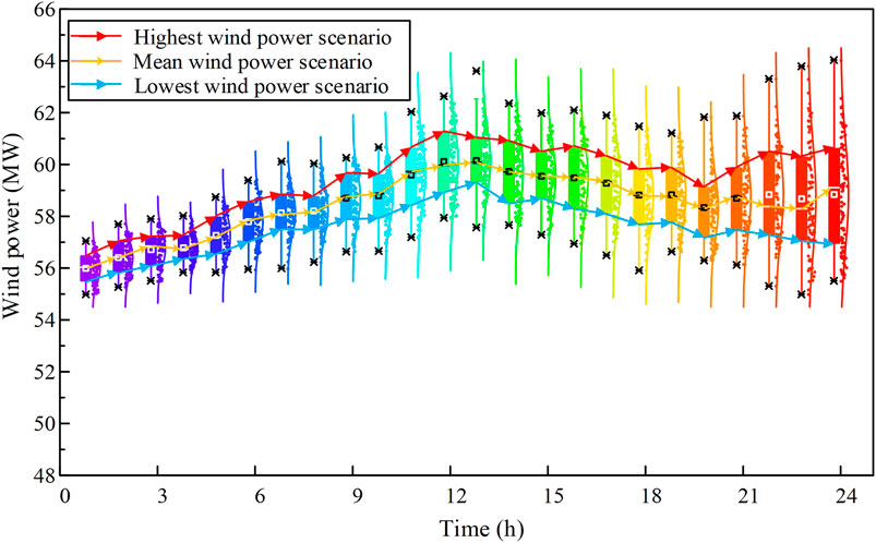
FIGURE 3. Generated ensemble forecasts of wind power of region 1.

FIGURE 4

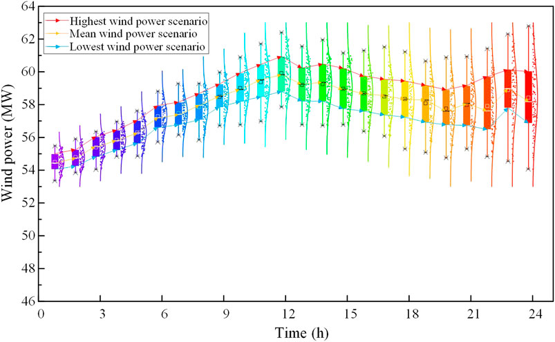
FIGURE 4. Generated ensemble forecasts of wind power of region 2.

FIGURE 5

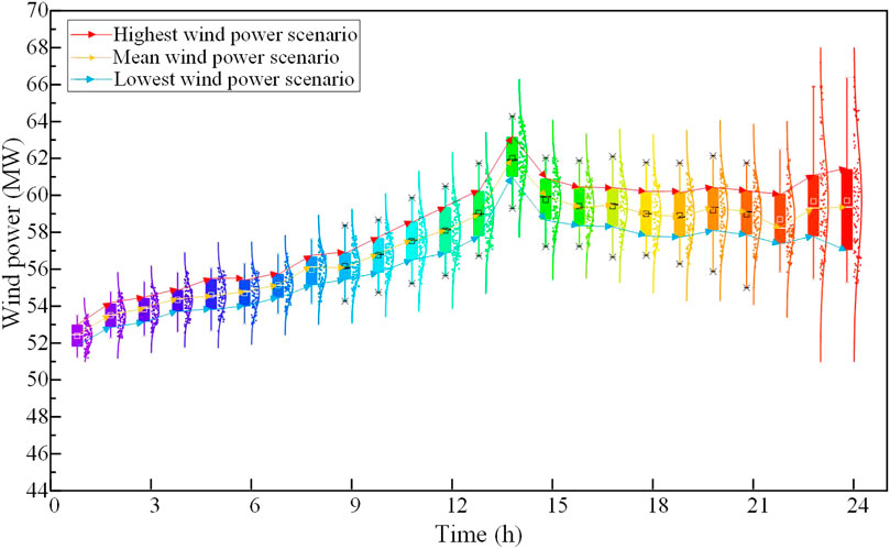
FIGURE 5. Generated ensemble forecasts of wind power of region 3.

FIGURE 6

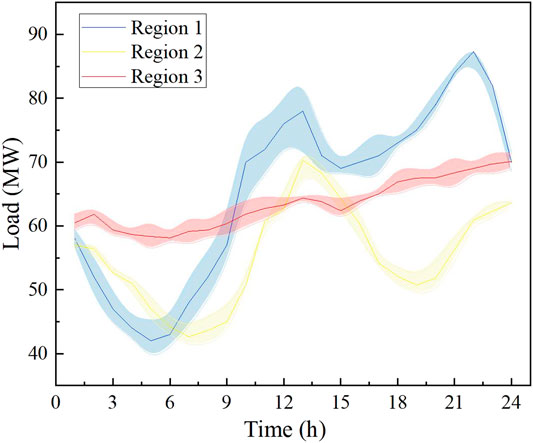
FIGURE 6. Flexible load of three regions.

Result Analysis

Trading Result in the Day-Ahead and Real-Time Stages

In the day-ahead stage, scenario 1 is taken as an example. The total net power of three regions, hydropower generation, trading power between multi-regions, and trading power of hydropower and multi-regions to the grid are shown in Figure 7.

FIGURE 7

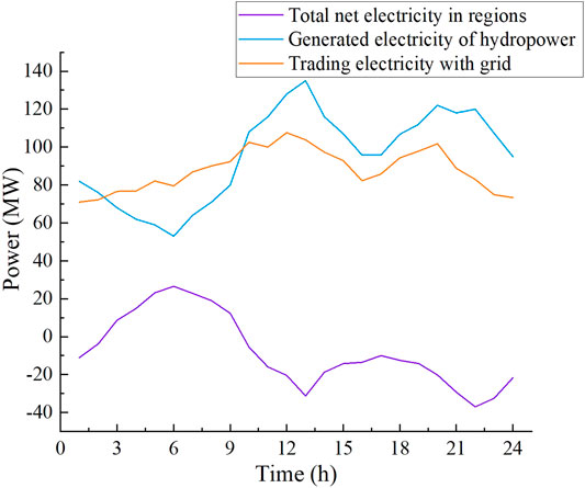
FIGURE 7. Trading power in the day-ahead stage.

As shown in Figure 7, when the regional total net power is negative, the value of hydropower output is greater than the value of power trading with a large power grid. It illustrates that part of the hydropower output is to supplement the power shortage in the region and part of the power is sold to the grid, therefore, the role of hydropower is demonstrated. When the regional total net power is positive, the output of hydropower is less than that of power trading with the grid. The regional excess power will be sold to the grid, and the hydropower generation will also be sold to the grid. Furthermore, the fluctuation of tie lines trading with the grid will be reduced after hydropower is added, which indicates that hydropower can suppress the fluctuation of wind power effectively. The maximum and mean values of tie-line volatility under the three scenarios are shown in Table 1.

TABLE 1

TABLE 1. Comparison of tie-line volatility.

As shown in Table 1, after adding hydropower, the tie line volatility would be decreased in each scenario, which prove the function of multi power operation. The average of maximal tie line volatility with hydropower is reduced by 0.2463 after adding hydropower, and the average of mean tie line volatility with hydropower is reduced by 0.1831 after adding hydropower, which indicates the positive role of hydropower. The harmful impact on the grid is reduced. In the day-ahead stage, the revenue of transaction between hydropower and three regions is shown in Figure 8.

FIGURE 8

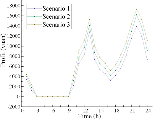
FIGURE 8. Revenue of transaction between hydropower and multi-regions.

As shown in Figure 8, the revenue of transaction between hydropower and multi-regions is the highest under scenario 3. The revenue under scenario 1 is the lowest because of the minimum wind power output in scenario 3 and the additional hydropower output needed to supplement the regional power shortage. From 3:00 to 9:00, the revenue is zero, which indicates that the regions do not trade with hydropower. The regions and hydropower experience shortage of power or have excess power. Thus, they would purchase or sell power from the grid. From 11:00 to 15:00 and 21:00 to 23:00, the trading power suddenly increases because of the increase of load that residents use during this period. In the day-ahead stage, the revenues of each region when the three regions trade with one another are shown in Figure 9. The yellow column represents the revenue of region 1, the green column represents the revenue of region 2, and the purple column represents the revenue of region 3.

FIGURE 9

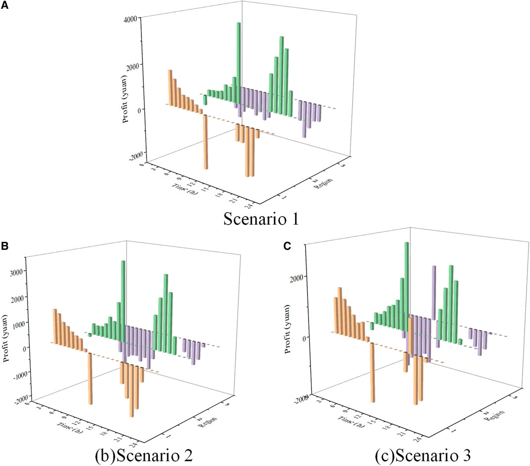
FIGURE 9. Revenues of each region when the three regions trade with one another under scenario 1.

As shown in Figure 9, in the first several hours of the day, the revenue of regions 1 and 2 is positive, and the revenue of region 3 is negative. It illustrates that the wind power output in regions 1 and 2 is greater than the corresponding load and the wind power output in region 3 is less than the load. Thus, the excess power in region 1 is sold to region 3. From 11:00 to 16:00 and 22:00 to 24:00, the revenue of the three regions is zero, which illustrates that not trading occurs among regions at theses time, the regions all are in a state of excess or shortage of power, and they need to purchase or sell power from hydropower or grid to overcome the regional imbalance between the power supply and the load. From 17:00 to 21:00, the revenue of regions 1 and 3 is negative, and the revenue of region 2 is positive, illustrating that regions 1 and 3 are in the state of power shortage and region 2 has excess power. The sum of the income of the three regions is zero, meeting the balance of income and expenditure. In the real-time stage, the net power of regions in the day-ahead and real-time stages, the generated power of pumped storage, and the trading power with the grid are shown in Figures 10–12. The deviation of power between the day-ahead and real-time stages is shown by the yellow shadow, and the deviation of power between the output of pumped storage and the trading power of the grid is shown by the blue shadow.

FIGURE 10

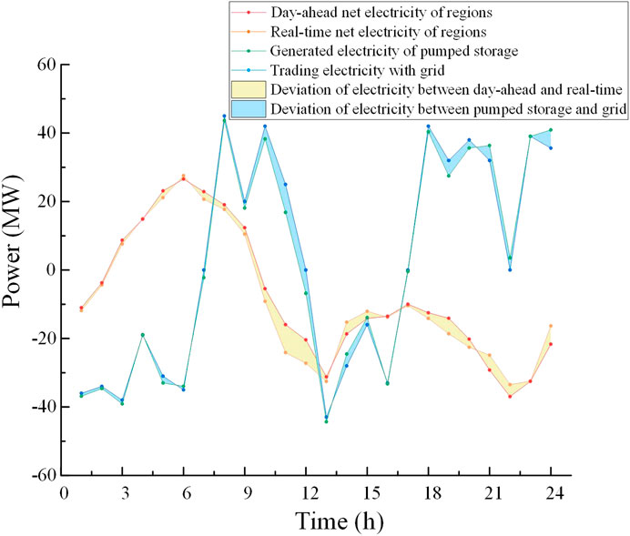
FIGURE 10. Trading power in the real-time stage of scenario 1.

FIGURE 11

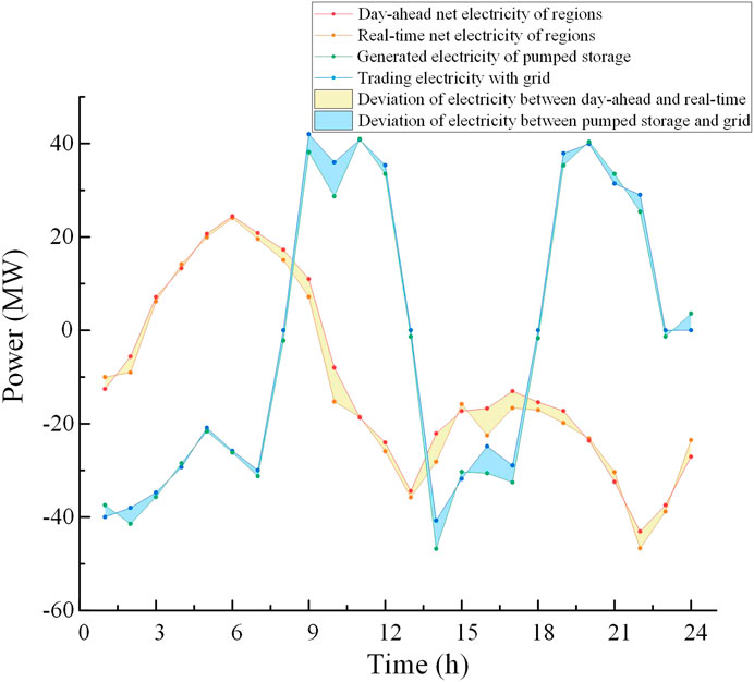
FIGURE 11. Trading power in the real-time stage of scenario 1.

FIGURE 12

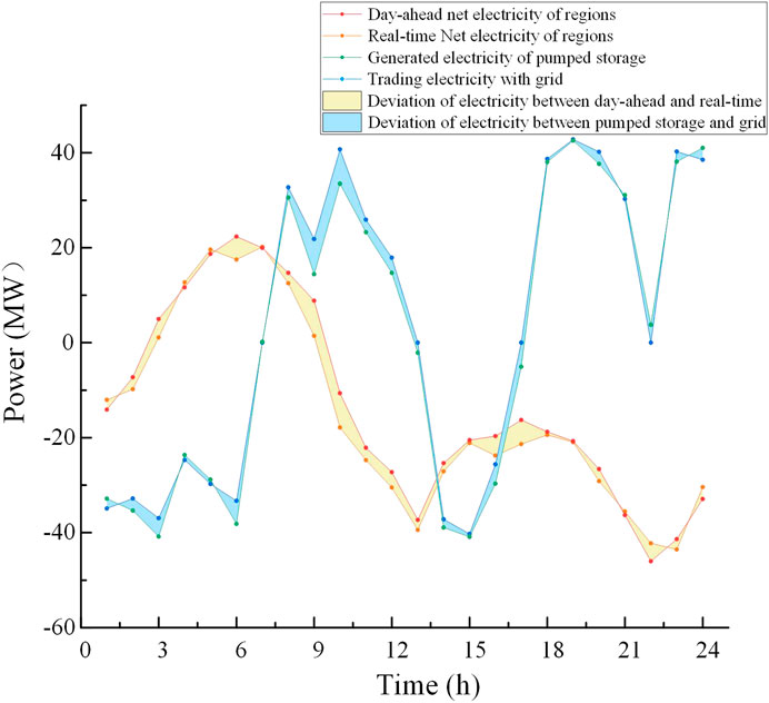
FIGURE 12. Trading power in the real-time stage of scenario 1.

As shown in Figures 10–12, the total net power of regions between the day-ahead and real-time stages has some deviation. When the total net power of regions in the real-time stages is more than that in the day-ahead stage, the generation of pumped storage is less than the trading power with the grid, which illustrates that the excess power caused by forecasting error and the generation of pumped storage would be sold to the grid. When the total net power of regions in the real-time stage is less than that in the day-ahead stage, the generation of pumped storage is more than the trading power with the grid, one part of the pumped storage generation is sold to the grid, and another part of the pumped storage generation is used to make up the shortage of power in regions.

Benefit Allocation

The benefit allocation method based on the traditional Shapley value only considers the number of power traders. The positive effects of hydropower and pumped storage on wind power are not considered, for example, stabilizing wind generation fluctuation, reducing the fluctuation of tie line with grid, and supplementing the power shortage caused by the uncertainty of wind power. Thus, this section compares the basic Shapley value method and the improved Shapley value method.

Benefit Allocation Result by Traditional Shapley Value Method

The results of different members’ benefits in the day-ahead and real-time stages, which are calculated by Eqs. 7, 8, are shown in Table 2. Symbols {1}, {2}, {3}, {4}, and {5} represent regions 1, 2, 3, hydropower, and pumped storage, respectively. The total benefit after cooperation is greater than the sum of individual benefits of each member before cooperation. The constraints of the cooperative game are satisfied.

TABLE 2

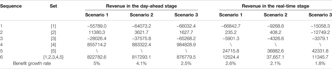
TABLE 2. Result of benefit allocation.

Improved Benefit Allocation Method

To show the performance of risk factor and cost factor in benefit allocation intuitively, the weighting coefficients of two factors are 1/2. Taking scenario 1 as an example, the benefit allocation results after adding the risk and cost factors are shown in Table 3.

TABLE 3

TABLE 3. Comparison of revenue by different benefit allocation methods.

As shown in Table 3, in the day-ahead stage, compared with the traditional Shapley method, the benefits of the three regions are reduced by 220.2, 310.2, and 680.2 yuan. The benefit of hydropower is increased by 1210.6 yuan. In the real-time stage, the benefit of pumped storage is also increased, which is in line with their role. The addition of hydropower and pumped storage has suppressed the fluctuation of renewable energy in regions but has lost part of its interests, which has a great risk. However, the benefit allocation scheme based on the traditional Shapley value method ignores the positive effects of hydropower and pumped storage. The improved Shapley method can promote the cooperation of all participants, and the allocation scheme is more reasonable.

Taking the day-ahead stage as an example, compared with the situation of noncooperation, the benefits of region 1, region 2, region 3, and hydropower are increased by 55230.9, 7035.28, 14637.8, and 12599.58 yuan, respectively. Considering the risk factor, the benefits of region 1, region 2, region 3, and hydropower are increased by 5010.7, 6725.06, 13957.6, and 13810.2 yuan, respectively. The benefit of each region and hydropower before and after adding hydropower in cooperation is shown in Figures 13–15.

FIGURE 13

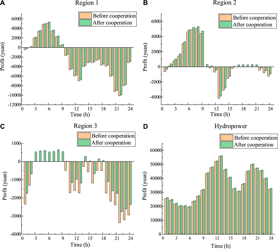
FIGURE 13. Comparison of benefit before and after adding hydropower.

FIGURE 14

FIGURE 14. Comparison of benefit before and after adding hydropower under scenario 2.

FIGURE 15

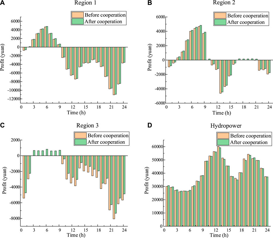
FIGURE 15. Comparison of benefit before and after adding hydropower under scenario 1.

As shown in Figures 13–15, the revenue of each participant after cooperation is greater than that before cooperation, which proves the rationality and effect of the cooperation. The revenue of the three regions is positive or negative in one day, which indicates that the difference between wind power output and load is fluctuating. When the revenue of a region is negative, it illustrates that power shortage is experienced after three regions trade with each other, and power should be purchased from the grid. When the revenue of a region is positive, which illustrates that the region has excess power, excess power would be sold to the grid. From 17:00 to 21:00 in region 2, the revenue of the region before adding hydropower is zero, which illustrates that the power shortage or excess in this region is just balanced by the other two regions, and no excess power would be traded with the grid.

Conclusion

In this study, the framework of two-stage dispatching about wind power, which contains the day-ahead and real-time stages, is proposed. The MMFE is used to generate synthetic ensemble wind power forecasts. The forecasted values show that the uncertainty of wind power forecasting would be increased over time, which is coincident with the actual situation, and the rationality of the proposed MMFE model is proven. Three typical scenarios are selected for analysis. In the day-ahead stage, the regions trade with one another. If excess power is generated, it is sold to the grid, but if a power shortage is experienced, hydropower would provide power. Based on the first-stage optimization, in the real-time stage, deviations of wind power output and load between the day-ahead stage and the real-time stage are observed because of their uncertainty. The pumped storage, which has the advantages of flexible schedulability, is used to make up for the shortage of power or purchase the excess power caused by the deviation. In the day-ahead stage, after adding hydropower for cooperation, the revenue of regions and hydropower all increase, and the average growth of the revenue is 3.87%. In the real-time stage, after adding the pumped storage, the revenue of all participants increase, and the average growth of the revenue is 2.17%, which proves the positive effect of hydropower and pumped storage. Considering the positive effect, the region should give some economic compensation to hydropower and pumped storage. An improved Shapley value method is proposed for benefit allocation. The risk and cost factors are added to the traditional Shapley method. Compared with the traditional Shapley method, the allocated benefit of hydropower and pumped storage is higher, which is more in line with the actual situation.

Data Availability Statement

The original contributions presented in the study are included in the article/Supplementary Material, further inquiries can be directed to the corresponding authors.

Author Contributions

SH, YX: Conceptualization, Methodology; SH: Writing-Original draft preparation; JuL: Supervision; YX, JiL, CL: Writing-Reviewing and Editing.

Conflict of Interest

Author JiL was employed by the Southwest Electric Power Design Institute Co., Ltd. Of China Power Engineering Consulting Group. Author CL was employed by the State Grid Sichuan Electric Power Research Institute.

The remaining authors declare that the research was conducted in the absence of any commercial or financial relationships that could be construed as a potential conflict of interest.

Acknowledgments

This work was supported by the National Key R&D Program of China (2018YFB0905200) and the National Natural Science Foundation of China (51807127).

References

Bayon, L., Grau, J., Ruiz, M., and Suarez, P. (2016). A comparative economic study of two configurations of hydro-wind power plants. Energy 112 (1), 8–16. doi:10.1016/j.energy.2016.05.133

CrossRef Full Text | Google Scholar

Bird, L., Lew, D., Milligan, M., Carlini, E., Estanqueiro, A., Flynn, D., et al. (2016). Wind and solar energy curtailment: a review of international experience. Renew. Sust. Energy Rev. 65, 577–586. doi:10.1016/j.rser.2016.06.082

CrossRef Full Text | Google Scholar

Biswas, P., Suganthan, P., Qu, B., and Amaratunga, G. (2018). Multiobjective economic-environmental power dispatch with stochastic wind-solar-small hydro power. Energy 150, 1039–1057. doi:10.1016/j.energy.2018.03.002

CrossRef Full Text | Google Scholar

Denault, M., Dupuis, D., and Couture-Cardinal, S. (2009). Complementarity of hydro and wind power: improving the risk profile of energy inflows. Energy Policy 37 (12), 5376–5384. doi:10.1016/j.enpol.2009.07.064

CrossRef Full Text | Google Scholar

Gebretsadik, Y., Fant, C., Strzepek, K., and Arndt, C. (2016). Optimized reservoir operation model of regional wind and hydro power integration case study: Zambezi basin and South Africa. Appl. Energy 161, 574–582. doi:10.1016/j.apenergy.2015.09.077

CrossRef Full Text | Google Scholar

Heath, D., and Jackson, P. (1994). Modeling the evolution of demand forecasts with application to safety stock analysis in production/distribution systems. IIE Trans. 26 (3), 17–30. doi:10.1080/07408179408966604

CrossRef Full Text | Google Scholar

International Energy Agency (2018). Renewables 2018: analysis and forecasts to 2023, executive summary. Availble at: https://www.iea.org/reports/renewables-2018 (Accessed May 01, 2020).

Google Scholar

Jakub, J., Mikulik, J., Krzywda, M., Ciapała, B., and Janowski, M. (2018). Integrating a wind- and solar-powered hybrid to the power system by coupling it with a hydroelectric power station with pumping installation. Energy 144, 549–563. doi:10.1016/j.energy.2017.12.011

CrossRef Full Text | Google Scholar

Javed, M. S., Ma, T., Jurasz, J., and Amin, M. (2020). Solar and wind power generation systems with pumped hydro storage: review and future perspectives. Renew. Energy 148, 176–192. doi:10.1016/j.renene.2019.11.157

CrossRef Full Text | Google Scholar

Kristiansen, M., Korpas, M., and Svendsen, H. (2018). A generic framework for power system flexibility analysis using cooperative game theory. Appl. Energy 212, 223–232. doi:10.1016/j.apenergy.2017.12.062

CrossRef Full Text | Google Scholar

Lasemi, M., and Arabkoohsar, A. (2020). Optimal operating strategy of high-temperature heat and power storage system coupled with a wind farm in energy market. Energy 210, 118545. doi:10.1016/j.energy.2020.118545

CrossRef Full Text | Google Scholar

Lee, D., and Wang, L. (2008). Small-signal stability analysis of an autonomous hybrid renewable Energy power generation/energy storage system part I: time-domain simulations. IEEE Trans. Energy Convers. 23 (1), 311–320. doi:10.1109/tec.2007.914309

CrossRef Full Text | Google Scholar

Li, F., and Qiu, J. (2016). Multi-objective optimization for integrated hydro-photovoltaic power system. Appl. Energy 167 (1), 377–384. doi:10.1016/j.apenergy.2015.09.018

CrossRef Full Text | Google Scholar

Li, J., Zhou, J., and Chen, B. (2020). Review of wind power scenario generation methods for optimal operation of renewable energy systems. Appl. Energy 280, 115992. doi:10.1016/j.apenergy.2020.115992

CrossRef Full Text | Google Scholar

Liggett, T., and Rumelt, L. (2009). The asymptotic shapley value for a simple market game. Econ. Theor. 40 (2), 333–338. doi:10.1007/s00199-008-0374-4

CrossRef Full Text | Google Scholar

Liu, Z., Zhang, Z., Zhuo, R., and Wang, X. (2019). Optimal operation of independent regional power grid with multiple wind-solar-hydro-battery power. Appl. Energy 235 (1), 1541–1550. doi:10.1016/j.apenergy.2018.11.072

CrossRef Full Text | Google Scholar

Lopes, V., and Borges, C. (2014). Impact of the combined integration of wind generation and small hydropower plants on the system reliability. IEEE Trans. Sust. Energy 6 (3), 1–9. doi:10.1109/TSTE.2014.2335895

CrossRef Full Text | Google Scholar

Panda, A., Tripathy, M., Barisal, A., and Prakash, T. (2017). A modified bacteria foraging based optimal power flow framework for hydro-thermal-wind generation system in the presence of STATCOM. Energy 124 (1), 720–740. doi:10.1016/j.energy.2017.02.090

CrossRef Full Text | Google Scholar

Reddy, S. (2017). Optimal scheduling of thermal-wind-solar power system with storage. Renew. Energy 101, 1357–1368. doi:10.1016/j.renene.2016.10.022

CrossRef Full Text | Google Scholar

Schmidt, J., Cancella, R., and Pereira, A. (2016). An optimal mix of solar PV, wind and hydro power for a low-carbon electricity supply in Brazil. Renew. Energy 85, 137–147. doi:10.1016/j.renene.2015.06.010

CrossRef Full Text | Google Scholar

Shahriari, M., Cervone, G., Clemente-Harding, L., and Delle Monache, L. (2020). Using the analog ensemble method as a proxy measurement for wind power predictability. Renew. Energy 146, 789–801. doi:10.1016/j.renene.2019.06.132

CrossRef Full Text | Google Scholar

Shayesteh, E., Amelin, M., and Soder, L. (2016). Multi-station equivalents for short-term hydropower scheduling. IEEE Trans. Power Syst. 31 (6), 4616–4625. doi:10.1109/tpwrs.2016.2515162

CrossRef Full Text | Google Scholar

Shen, J., Cheng, C., Zhang, X., and Zhou, B. (2018). Coordinated operations of multiple-reservoir cascaded hydropower plants with cooperation benefit allocation. Energy 153 (15), 509–518. doi:10.1016/j.energy.2018.04.056

CrossRef Full Text | Google Scholar

Tan, Z., Song, Y., Zhang, H., and Shang, J. (2013). Joint delivery system of large-scale wind power and thermal power generation and its profit distribution model. Autom. Electr. Power Syst. 37 (23), 63–70. doi:10.7500/APES2013.01.123

Google Scholar

Turk, A., Wu, Q., Zhang, M., and Stergaard, J. (2020). Day-ahead stochastic scheduling of integrated multi-energy system for flexibility synergy and uncertainty balancing. Energy 196, 117130. doi:10.1016/j.energy.2020.117130

CrossRef Full Text | Google Scholar

Wang, X., Mei, Y., Kong, Y., Lin, Y., and Wang, H. (2017). Improved multi-objective model and analysis of the coordinated operation of a hydro-wind-photovoltaic system. Energy 134, 813–839. doi:10.1016/j.energy.2017.06.047

CrossRef Full Text | Google Scholar

Wu, Z., Zhou, M., Yao, S., Li, G., Zhang, Y., and Liu, X. (2019). Optimization operation strategy of wind-storage coalition in spot market based on cooperative game theory. Power Syst. Technol. 43 (8), 2815–2824. doi:10.13335/j.1000-3673.pst.2019.0534

Google Scholar

Xu, B., Chen, D., Venkateshkumar, M., Xiao, Y., Yue, Y., Xing, Y., et al. (2019). Modeling a pumped storage hydropower integrated to a hybrid power system with solar-wind power and its stability analysis. Appl. Energy 248 (15), 446–462. doi:10.1016/j.apenergy.2019.04.125

CrossRef Full Text | Google Scholar

Yang, S., Tan, Z., Lin, H., Li, P., De, G., Zhou, F., et al. (2020). A two-stage optimization model for park integrated energy system operation and benefit allocation considering the effect of time-of-use energy price. Energy 195, 117013. doi:10.1016/j.energy.2020.117013

CrossRef Full Text | Google Scholar

Zhang, C., Zhao, Z., Zhuang, J., and Wang, B. (2017). Risk-aware short term hydro-wind-thermal scheduling using a probability interval optimization model. Appl. energy 189, 534–554. doi:10.1016/j.apenergy.2016.12.031

CrossRef Full Text | Google Scholar

Zhang, H., Lu, Z., Hu, W., Wang, Y., Dong, L., and Zhang, J. (2019). Coordinated optimal operation of hydro-wind-solar integrated systems. Appl. Energy 242, 883–896. doi:10.1016/j.apenergy.2019.03.064

CrossRef Full Text | Google Scholar

Zhang, H., Lu, Z., Hu, W., Wang, Y., Dong, L., and Zhang, J. (2019). Coordinated optimal operation of hydro-wind-solar integrated systems. Appl. Energy 242, 883–896. doi:10.1016/j.apenergy.2019.03.064

CrossRef Full Text | Google Scholar

Zhang, Y., Wang, J., and Wang, X. (2014). Review on probabilistic forecasting of wind power generation. Renew. Sust. Energy Rev. 32, 255–270. doi:10.1016/j.rser.2014.01.033

CrossRef Full Text | Google Scholar

Zhao, T., Cai, X., and Yang, D. (2011). Effect of streamflow forecast uncertainty on real-time reservoir operation. Adv. Water Resour. 34 (4), 495–504. doi:10.1016/j.advwatres.2011.01.004

CrossRef Full Text | Google Scholar

Zhou, J., Peng, Y., Wang, C., and Yuan, L. (2016). Short-term hydro-thermal-wind complementary scheduling considering uncertainty of wind power using an enhanced multi-objective bee colony optimization algorithm. Energy Convers. Manag. 123, 116–129. doi:10.1016/j.enconman.2016.05.073

CrossRef Full Text | Google Scholar