Data-Driven-Based Forecasting of Two-Phase Flow Parameters in Rectangular Channel

In the current nuclear reactor system analysis codes, the interfacial area concentration and void fraction are mainly obtained through empirical relations based on different flow regime maps. In the present research, the data-driven method has been proposed, using four machine learning algorithms (lasso regression, support vector regression, random forest regression and back propagation neural network) in the field of artificial intelligence to predict some important two-phase flow parameters in rectangular channels, and evaluate the performance of different models through multiple metrics. The random forest regression algorithm was found to have the strongest ability to learn from the experimental data in this study. Test results show that the prediction errors of the random forest regression model for interfacial area concentrations and void fractions are all less than 20%, which means the target parameters have been forecasted with good accuracy.

Introduction

In various industrial equipment of nuclear power systems, gas-liquid two-phase flow phenomenon is widespreaded. Research on the two-phase flow plays an important role in improving the safety and operational reliability of evaluation system equipment. At present, in traditional commercial nuclear reactor system safety analysis softwares such as Reactor Excursion and Leak Analysis Program (RELAP) 5 (Martin, 1995) and CATHARE (Barre and Bernard, 1990), two-fluid models are widely used in the two-phase flow and heat transfer processes. In order to improve the calculation accuracy of the two-fluid model, it is necessary to provide more accurate closure models for the two-fluid model, and the interface transport term must be accurately simulated (Guo, 2002). The interface transport term can be expressed as the product of the interfacial area concentration and interfacial transport driving force where the interfacial area concentration is defined as the interfacial area per unit mixture volume, which represents the effective area for mass-energy exchange between different phases. For two-phase flow system, the interfacial area concentration and void fraction are also two of the most important parameters.

In view of the importance of parameters such as the interfacial area concentration, a variety of measurement methods have been developed to obtain experimental data, such as probe method, high-speed camera method, chemical method, etc., and different types of empirical correlations have been established based on a large amount of data (Ishii, 1975; Kocamustafaogullari and Ishii, 1995; Su, 2013). However, the scope of application of these empirical correlations is relatively limited. Moreover, the acquisition of experimental data is costly with typical local features.

In recent years, with the continuous development of computer hardware, computing power as well as data collection and storage technology, artificial intelligence technology has made a qualitative leap in emerging applications and development in various fields. However, in the field of engineering, especially nuclear engineering, the application of data-driven methods, whether it is fault diagnosis, equipment health management or other aspects, is still subject to certain restrictions. There are many prediction and analysis methods based on data-driven routes, including machine learning, deep learning, information fusion, statistical analysis methods, signal processing analysis methods, etc. (Gammerman, 1996).

Machine learning (including deep learning), as known as the cornerstone of artificial intelligence technology, has become a popular research field in recent years. Implementation of machine learning completely starts from collecting operating parameters, constructing data analysis models through the learning of historical data, and then is conducted by using the trained models to give a predicted output for the actual input parameters. A review of the research and development status of learning-based methods used in reactor health and management, radiation detection and protection, as well as optimization illustrated that, at present, more and more researchers in various fields of nuclear science are showing enthusiasm for the data-driven parameters or states predictions, and these methods have become more practical with the rising of deep learning and other techniques in the past decade (Gomez-Fernandez et al., 2020). The most important application of machine learning in reactor health management is to use sensor data for parameter prediction and state classification to perform tasks such as stateful inspection, fault diagnosis, and life prediction control. Among them, Tennessee Valley Authority Sequoyah Nuclear Plant uses the artificial neural network to determine the variables that affect the heat rate and thermal performance (Guo and Uhrig, 1992). Advanced optimization algorithms are used to estimate local power peaking factor estimation in nuclear fuel (Montes et al., 2009). Nuclear reactor thermal-hydraulic research area has also shown interests in the application of machine learning: for instance, flow regime identification (Tambouratzis and Pàzsit, 2010), prediction of two-phase mixture density (Lombardi and Mazzola, 1997) and expert decision support systems trained by deep neural networks/long short-term memory which is developed to predict the progression of LOCA (Radaideh et al., 2020).

The data-driven method is more desired where the prediction task is more complex due to the enhancement of the data availability and reduce computational difficulty in some cases. In the present work, data-driven method is introduced in predicting two-phase flow parameters in rectangular channels, namely interfacial area concentration and voidfraction, by using four machine learning models: lasso regression, support vector regression, random forest regression and back propagation neural network. Additionally, the performance of four models for different parameters prediction will be discussed and compared in the present work. The remaining sections of this paper are organized as follows: Section Data Acquisition describes the experimental equipment and the process of data acquisition. The algorithms adopted in this paper are presented in Section Algorithm. The methods and test results of this paper are presented in Section Methodology. The result is further analyzed and discussed in Section Discussion. The conclusions drawn from this study are given in Section Conclusion.

Data Acquisition

Introduction to the Experimental System

This experimental platform is shown in Figure 1, which can carry out the research of the vertical air-water two-phase flow in the channels with various cross-sectional area under normal temperature and pressure conditions. Figure 1 is a schematic diagram of the experimental system, and Figure 2 is the scene photo of the experimental system.

FIGURE 1

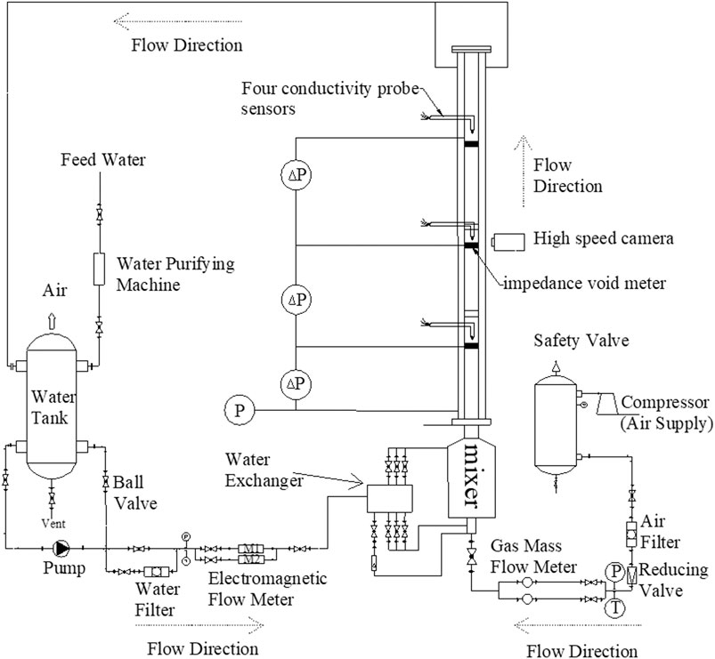
FIGURE 1. Schematic diagram of the experimental loop system.

FIGURE 2

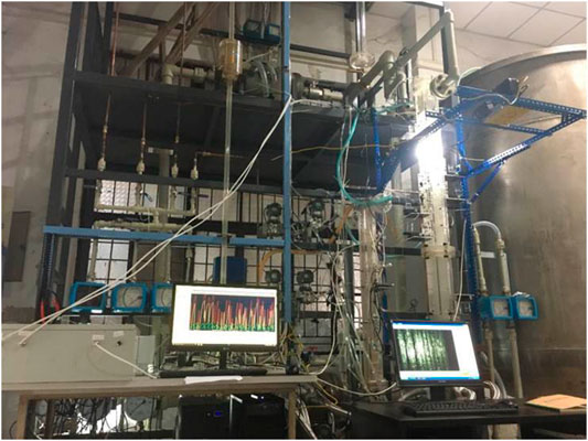
FIGURE 2. A photograph of experimental system.

The experimental platform is mainly composed of water supply system, air supply system, air-water mixer, experimental section, instrumentation, and data acquisition system. The main part of experimental device is a rectangular channel with the total length of the experimental section about 1,500 mm and the channel size of 66 × 6 mm. The experimental section is all processed and bonded with transparent acrylic material for experimental observation. Four pressure measuring setpoints are distributed in the axial position, namely the entrance and three positions of the impedance void meters. The experiment uses three sets of electrodes as the void meters, and the measurement data can also be used for flow pattern identification and calibration. Conductivity probes are arranged at the position of the void meters to obtain local physical parameters such as the interfacial area concentration, void fraction, and bubble velocity. In order to provide a clear and intuitive explanation for the measurement data of the void meters and the conductivity probe, a high-speed camera is placed near the void meters and the conductivity probes. The probe measuring setpoints are arranged in the radial position with 30 ∼ 31 measuring setpoints, and the measuring setpoint arrangement positions are shown in Figure 3, where X represents the radial distance of the probes.

FIGURE 3

FIGURE 3. The schematic of probe measuring setpoints in the radial position.

The specific experimental parameter ranges are shown in Table 1 and the range of experimental conditions is shown in Figure 4. The experimental conditions are obtained by different flow regime. Black dots represent bubbly flow, red dots represent slug flow, green dots represent churn-turbulent flow, and blue dots represent annular flow. As far as the maximum uncertainty of the experiment is concerned, the values of liquid flow measurements, gas flow measurements, probe voltage acquisition, probe tip size measurements, and void meters are 3.2, 2.45, 1.23, 2 and 2.01%, respectively.

TABLE 1

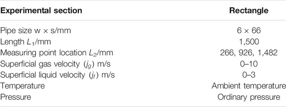
TABLE 1. Experimental parameters of the rectangular channel.

FIGURE 4

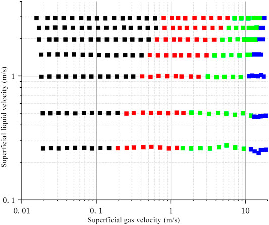
FIGURE 4. Schematic diagram of experimental conditions.

Algorithm

This chapter introduces the machine learning algorithms and principles used in this research, including lasso regression (LR), support vector regression (SVR), random forest regression (RFR) and back propagation neural network (BPNN).

Lasso Regression

Multiple linear regression refers to the study of the influence of changes in independent variables ${\mathit{x}}_1,{\mathit{x}}_2,\dots ,{\mathit{x}}_{\mathit{m}}$ on dependent variable $\mathit{y}$. The model can be expressed as:

$y={\beta }_0+{\beta }_1{x}_1+{\beta }_2{x}_2+\cdots +{\beta }_m{x}_m+\epsilon ,(1)$

where ${\beta }_0,{\beta }_1,{\beta }_2,\dots ,{\beta }_m$ are unknown coefficients and $\epsilon$ is the independent identically distributed normal error.

In order to solve Eq. 1, methods such as least squares are usually used to estimate the parameters of the regression model from the perspective of error fitting, and the optimization goal can be expressed in matrix form as:

${\beta }^{\text{*}}={\text{argmin}}_{\beta }\frac{1}{m}{\Vert y-X\beta \Vert }^2(2)$

However, the least squares method still has some shortcomings when facing multiple input features, for instance its unbiased estimation characteristics will lead to large variance. Lasso regression (least absolute shrinkage and selection operator) was proposed by Robert Tibshirani in 1996 based on Leo Breiman’s non-negative garrote (Breiman, 1995; Tibshirani, 1996). It is a shrinkage estimation algorithm and its basic idea is to minimize the residual sum of squares under the constraint that the sum of the absolute values of the regression coefficients is less than a constant, and to reduce the non-zero components in the regression coefficients, thereby improving the accuracy of the prediction and the interpretability of the regression model. The objective equation of the lasso algorithm is:

${\beta }^{\text{*}}={\text{argmin}}_{\beta }\frac{1}{m}{\Vert y-X\beta \Vert }^2+\lambda \Vert \beta \Vert (3)$

where $y$ is target variable, $\beta$ is regression coefficient vector, $X$ is the data matrix corresponding to explanatory variables and $\lambda$ is the penalty parameter. Lasso regression is a quadratic programming problem that the solving algorithms include shooting algorithm, homotopy algorithm, etc.

Support Vector Regression

Support vector machine was originally used to deal with pattern recognition problems (Vapnik, 1998), but its sparse solution and good generalization make it suitable for regression problems. The generalization from SVM to SVR is accomplished by introducing an $\epsilon$-tube, which reformulates the optimization problem to find the best approximation of the continuous-valued function, while balancing complexity and prediction error of prediction model. For nonlinear support vector machine regression, the basic idea is to map the data $x$ to the high-dimensional Hilbert space $\varphi \left(x\right)$ through a nonlinear mapping $\varphi$, and seek the regression linear hyperplane in this space, thereby solving the highly non-linear problems in the low-dimensional space. The linear model in the high-dimensional feature space is constructed as follows:

$f\left(x\right)=\langle w\cdot \varphi \left(x\right)\rangle +b,(4)$

where $w$ is the weight vector, $b$ is the bias constant and $\langle w\cdot \varphi \left(x\right)\rangle$ is the inner product of the feature space. The optimal hyperplane regression estimation function is converted as follows:

$f\left(x\right)={\displaystyle {\sum }_{i=1}^n\left(a_i-a_i^{\text{*}}\right)k\left(x_i,x_j\right)}+b,(5)$

where $a_i$ and $a_i^{\text{*}}$ are lagrange multipliers, $k\left(x_i,x_j\right)=\varphi \left(x_i\right)\cdot \varphi \left(x_j\right)$ is kernel function. The types of kernels include polynomial kernel, Gauss radial basis function kernel, and sigmoid kernel, etc. while radial basis function kernel (RBF kernel) is selected as the kernel function in the present study because in some researches RBF kernel has been pointed out be appropriate for nonlinear systems, which is expressed as (Zhang and Li, 2006):

$k\left(x_i,x_j\right)=e^{-\left({\Vert x_i-x_j\Vert }^2÷{\sigma }^2\right)}(6)$

Random Forest Regression

Random forest is an ensemble algorithm proposed by Breiman in 2001 (Breiman, 2001a; Breiman, 2001b). In general, the random forest shown in Figure 5 is composed of multiple CART decision trees, which conducts classification or regression through bagging (bootstrap aggregating). The main idea of random forest regression method (RFR) is to extract multiple samples from the original sample, build a decision tree for each sample, and then use the average of all decision tree predictions as the final prediction result. RFR was pointed out that it has the advantages of fast training speed, strong adaptability to high-dimensional data sets, and strong robustness in the face of noise (Segal, 2004).

FIGURE 5

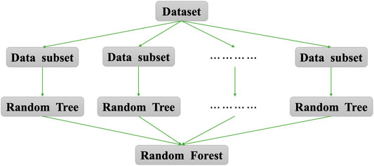
FIGURE 5. The structure of Ramdom Forest.

In principle, the random forest regression (RFR) is composed of a set of sub-decision trees $\left\{h\left(x,{\theta }_t\right),t=\mathrm{1,2,3},\dots T\right\}$, where ${\theta }_t$ is a random variable subject to independent and identical distribution, $x$ represents the independent variable, and $T$ represents the number of decision trees.

RFR uses the results of integrating multiple decision trees to take the mean value of $\left\{h\left(x,{\theta }_t\right)\right\}$ as the regression prediction result to eliminate the problems of overfitting and low precision of the decision tree model. The result is expressed as

$\overline{h}\left(x\right)=\frac{1}{T}{\displaystyle {\sum }_{t=1}^T\left\{h\left(x,{\theta }_t\right)\right\}}(7)$

The RFR algorithm implementation process is as follows:

(1) Bagging is used to randomly generate sample subsets.

(2) Use the idea of random subspace by randomly extracting features, splitting nodes and building a regression sub-decision tree.

(3) Repeat the above steps to construct T regression decision subtrees to form a random forest (Pruning and other human intervention is not allowed in the process).

(4) Take the predicted values of $T$ sub-decision trees and take the mean as the final prediction result.

Back Propagation Neural Network

Artificial neural network is a widely parallel interconnected network composed of adaptable simple units; its organization can simulate the interactive response of the biological neural system to real world objects (Kohonen, 1988). In the development of artificial neural networks, the error back-propagation algorithm occupies an important place (McClelland et al., 1986). The network based on this algorithm is referred to as BP network, which consists of one input layer, at least one hidden layer, and one output layer. The usually constructed BP neural network is a three-layer network. For regression prediction, the output layer usually has only one neuron.

Given the training set $D=\left\{\left({\mathit{x}}_1,y_1\right),\left({\mathit{x}}_2,y_2\right),\dots ,\left({\mathit{x}}_{\mathit{m}},y_m\right)\right\}$, where ${\mathit{x}}_{\mathit{i}}\in {\mathrm{ℝ}}^d$, $y_i\in \mathrm{ℝ}$. Figure 6 shows a BP neural network with $d$ input neurons, one output neuron, and $q$ hidden layer neurons. The threshold of the output layer neuron is represented by $\theta$, and the threshold of the $h$-th neuron in the hidden layer is represented by ${\gamma }_h$. The connection weight between the i-th neuron in the input layer and the h-th neuron in the hidden layer is $v_{ih}$, and the connection weight between the h-th neuron in the hidden layer and the output layer neuron is ${\omega }_h$. The input received by the h-th neuron in the hidden layer is ${\alpha }_h={\displaystyle {\sum }_{i=1}^d{v}_{ih}{x}_i}$, and the input received by the output layer neuron is $\beta ={\displaystyle {\sum }_{h=1}^q{\omega }_h{b}_h}$, where $b_h$ is the output of the h-th neuron in the hidden layer.

FIGURE 6

FIGURE 6. Basic structure of BP neural network.

For training example $\left({\mathit{x}}_{\mathit{k}},y_k\right)$, assuming that the output of the neural network is ${\widehat{y}}_k\in \mathrm{ℝ}$, that is

${\widehat{y}}_k=f_2\left(\beta +\theta \right)(8)$

Then the mean-square error of the network on $\left({\mathit{x}}_{\mathit{k}},y_k\right)$ is

$E_k=\frac{1}{2}{\left({\widehat{y}}_k-y_k\right)}^2(9)$

For the hidden layer, we have

$b_h=f_1\left({\alpha }_h+{\gamma }_h\right)(10)$

where $f_1(\cdot )$ and $f_2(\cdot )$ are both activation functions. In consideration of regression prediction, $f_1(\cdot )$ in ourstudy is ReLU function, i.e.

$f_1\left(x\right)=\text{max}\left(0,x\right)(11)$

The function $f_2(\cdot )$ is preferable to the purelin function, i.e.

$f_2\left(x\right)=x(12)$

The BP algorithm is based on a gradient descent strategy and adjusts the parameters in the direction of the negative gradient of the target. For the error $E_k$, given the learning rate $\eta$, we have

$\Delta {\omega }_h=-\eta \frac{\partial E_k}{\partial {\omega }_h}=\eta \left(y_k-{\widehat{y}}_k\right)f_1\left({\alpha }_h+{\gamma }_h\right)(13)$

$\Delta \theta =-\eta \frac{\partial E_k}{\partial \theta }=\eta \left(y_k-{\widehat{y}}_k\right)(14)$

$\Delta v_{ih}=-\eta \frac{\partial E_k}{\partial v_{ih}}=\eta \left(y_k-{\widehat{y}}_k\right){\omega }_h{f}_1^{\prime }\left({\alpha }_h+{\gamma }_h\right)x_i(15)$

$\Delta {\gamma }_h=-\eta \frac{\partial E_k}{\partial {\gamma }_h}=\eta \left(y_k-{\widehat{y}}_k\right){\omega }_h{f}_1^{\prime }\left({\alpha }_h+{\gamma }_h\right)(16)$

The flow of BP algorithm is as follows:

(1) Set the network structure, input layer, hidden layer, output layer and learning rate $\eta$, where the output layer node number is set to 1;

(2) Randomly initialize the connection weight $v_{ih}$, ${\omega }_h$ and the threshold ${\gamma }_h$, $\theta$ in the network within the range of $\left(\mathrm{0,1}\right)$;

(3) Randomly select a training sample $\left({\mathit{x}}_{\mathit{k}},y_k\right)$, and calculate the output ${\widehat{y}}_k$ of the current sample according to the current parameters and Eq. 8;

(4) Calculate the weight correction $\Delta {\omega }_h$, $\Delta v_{ih}$ and the threshold correction $\Delta \theta$, $\Delta {\gamma }_h$ according to Eqs 13–16;

(5) Update connection weights and thresholds:

${\omega }_h\leftarrow {\omega }_h+\Delta {\omega }_h,$

$v_{ih}\leftarrow v_{ih}+\Delta v_{ih},$

$\theta \leftarrow \theta +\Delta \theta ,$

${\gamma }_h\leftarrow {\gamma }_h+\Delta {\gamma }_h.$

(1) Go back to step 3) until all the training data are input;

(2) Go back to steps 2)–6) until the stop condition is reached.

Methodology

Data Preprocessing

In two-phase flow, considering the difference between the bubbles of different shapes and sizes, the bubbles were usually categorized into two bubble groups: group-I represents small-dispersed and distorted bubbles, whereas group-II represents cap/slug/churn-turbulent bubbles. (Ishii et al., 2002). Therefore, the interfacial area concentrations and void fractions are described by different bubbles characteristics of group-I and group-II respectively. The present research is based on real experimental measurement data that selects the axial distance Z, the radial distance X, superficial gas velocity $J_g$ and superficial liquid velocity $J_f$ as input features, and takes group-I interfacial area concentration, group-II interfacial area concentration, group-I void fraction, and group-II void fraction as outputs.

Since the units and dimensions of each input parameter are not the same, the data needs to be standardized before modeling. In this study, the mean variance normalization method was used to make the processed data set conform to the standard normal distribution, with a standard deviation of 1 and a mean of 0. The specific formula is as follows:

$d_{norm}=\left(d-\mu \right)/\sigma ,(17)$

where $d_{norm}$ is the standardized data set, $d$ is the original data set, $\mu$ is the average value, and $\sigma$ is the standard deviation.

Model Performance Metrics

In this study, the coefficient of determination $\left(R^2\right)$, the root-mean-square error (RMSE) and the coefficient of variation (CV) were selected as evaluation indicators of model performances. Supposing a series of data sets $y_1,\dots ,y_n$ includes $n$ data points, and their corresponding model prediction values are $p_1,\dots ,p_n$.

The expression of the coefficient of determination $R^2$ is

${\text{R}}^2\equiv 1-\frac{{\displaystyle {\sum }_i{\left(y_i-p_i\right)}^2}}{{\displaystyle {\sum }_i{\left(y_i-\overline{y}\right)}^2}},(18)$

where the closer the value of ${\text{R}}^2$ is to 1, the better the effect of model fitting.

The expression of $\text{RMSE}$ is

$\text{RMSE}=\sqrt{\frac{1}{\text{m}}{\displaystyle \sum _{i=1}^m{\left(y_i-p_i\right)}^2}},(19)$

where $m$ represents the number of samples, and the smaller the value, the smaller the error between the model prediction result and the true value.

In order to introduce the concept of percentage error rate to further explore the performance of the model, this paper selects the coefficient of variation (CV) to describe the model. The expression of the CV is

$\text{CV}=\frac{\sqrt{\left(1/m\right){\displaystyle {\sum }_{i=1}^m{\left(y_i-p_i\right)}^2}}}{y}\times 100\%(20)$

When describing the model, the $\text{CV}$ for a model aims to describe the model fit in terms of the relative sizes of the squared residuals and outcome value. The range of CV is between 0 and 100%. The smaller $\text{CV}$ is, the more accurate the prediction of the model is.

Hyperparameters Tuning

In this study, the hyperparameter tuning process of four different models is implemented from using grid search method. The basic principle is to divide the interval of each parameter variable value into a series of small areas, and calculate the corresponding the target value (error in usual) determined by the combination of each hyperparameter variable values, and select the best one by one to obtain the minimum target value in the interval and its corresponding optimal hyperparameter. This method ensures that the search solution obtained is globally optimal or close to optimal. The hyperparameters optimization process in this study also considers the limits of the accuracy of the running results and the computational efficiency. However, the calculation time is not included in the model metric in this study.

For LR regression, the regularization parameter $\lambda$ from Eq. 3 is considered to be the most important indicator that affects the accuracy of the model. In theory, the larger the regularization parameter, the stronger the model’s robustness against collinearity. However, if the regularization parameter is selected too big, all parameters $\beta$ will be minimized, resulting in under-fitting. If the regularization parameter is selected too small, it will lead to improper solution to the over-fitting problem. When predicting the four sets of two-phase flow parameters, in order to expand the search for the appropriate range of $\lambda$, 50 sets of $\lambda$ were selected for model optimization: an arithmetic sequence between 0.0001 and 0.1 (including 25 numbers) and an arithmetic sequence between 0.1 and 100 (including 25 numbers).

For the RFR model, the number of trees in the forest, the maximum depth of the tree and random state are commonly considered to be the key parameters that affect the performance of the model. Due to the few dimensions of input variables in this study, another hyperparameter that is often considered, namely the number of features to consider when looking for the best split, defaults to the maximum value 4 in this study. The three hyperparameters mentioned above are optimized using grid searchwith bounds selected as:

• the number of trees with bound: 50–250

• the maximum depth of the tree: 7–12

• random state: 1–12

For the SVR model, the kernel function is the RBF kernel which is better for nonlinear problems. Three major hyperparameters are also optimized using grid search with bounds selected as follows:

• Kernel coefficient with bound: 0.001–0.1

• Regularization parameter with bound: 0.1–100

• Size of the kernel cache (MB): 10,000–50,000

Last but not least, for BPNN model, five major hyperparameters are optimized using grid search with bounds selected as follows:

• Batch size with bound: 512–1,024

• Epochs with bound:150–500

• Processing units: 64–128

• Learning rate: 0.001–0.05

• Activiation function: ReLU

The results of the optimum architecture of four models are listed in Table 2. It is worth mentioning that we directly selected ReLU, a piecewise linear function which is proven to be most effective for BP-NN (Nair and Hinton, 2010).

TABLE 2

TABLE 2. The selected hyperparameters for each output.

Model Training, Validation and Testing

The calculations of models were performed using an Apple laptop with Mac OS system (version 10.15), core Intel i5 5257U, 8 GB of RAM, and Intel Iris Graphics 6100 card with 1536 MB of the RAM. The utilization and implementation of the models in this study are done in the Python environment (Van Rossum and Drake, 1995).

For common machine learning problems, the data should be divided into training set, validation set and test set. The training set is used for model fitting, the validation set is used to adjust the hyperparameters of the model to prevent the model from overfitting and to make an initial assessment of the model's ability, and the test set is used to evaluate the generalization ability of the final model. In this study, all data were first divided into training set and test set at a ratio of 9:1. Cross-validation is selected as the method of model validation in the present work. Compared with the ordinary way with fixed validation set, cross-validation (Kohavi, 1995) contributes to obtain as much effective information as possible from the limited learning data. In general, the principle of cross-validation is to learn training samples from multiple directions, which can effectively avoid falling into local minimums and to a certain extent avoid over-fitting problems. In this study, the K-fold cross-validation method is used to achieve cross-validation whose idea is to divide the training set into k sub-samples, where a single sub-sample is retained as the data for the validation model, and the other k-1 samples are used for training. Cross-validation is conducted by repeating k times and each sub-sample is validated once. Hence, mean value of k-times’ validation, or other combination methods are used to obtain a single final estimate. In this study, the most used cross validation method, namely 10-fold cross-validation was selected (McLachlan et al., 2005). In this study, assuming that a group of corresponding inputs and outputs are regarded as a data set, the number of data sets is 3,146 in total.

Discussion

In the previous section, the route that four two-phase flow parameters obtained from rectangular channel experiments are modeled and predicted by LR, RFR, SVR, and BPNN is introduced in detail. Figures 7–10 respectively show the comparison between a part of the test set data and its corresponding real data. The blue line is the target data, that is, the true value while the orange-red line is the predicted value generated by the model. Each figure shows the comparison of the predictive capabilities of the four models for a single output. The unit of interfacial area concentration is $1/m$, and void fraction is a dimensionless parameter.

FIGURE 7

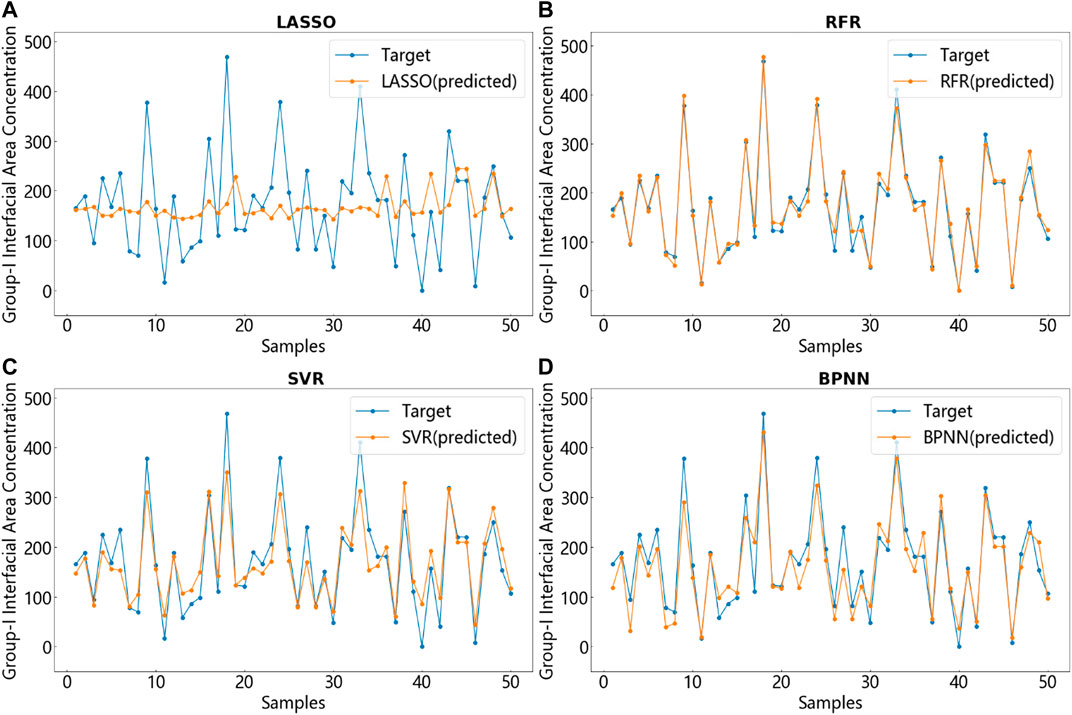
FIGURE 7. Prediction of the group-I interfacial area concentration using four models and comparison with target values. (A) LASSO. (B) RFR. (C) SVR (D) BPNN.

FIGURE 8

FIGURE 8. Prediction of the group-II interfacial area concentration using four models and comparison with target values. (A) LASSO. (B) RFR. (C) SVR (D) BPNN.

FIGURE 9

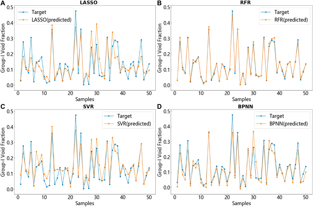
FIGURE 9. Prediction of the group-I void fraction using four models and comparison with target values. (A) LASSO. (B) RFR. (C) SVR (D) BPNN.

FIGURE 10

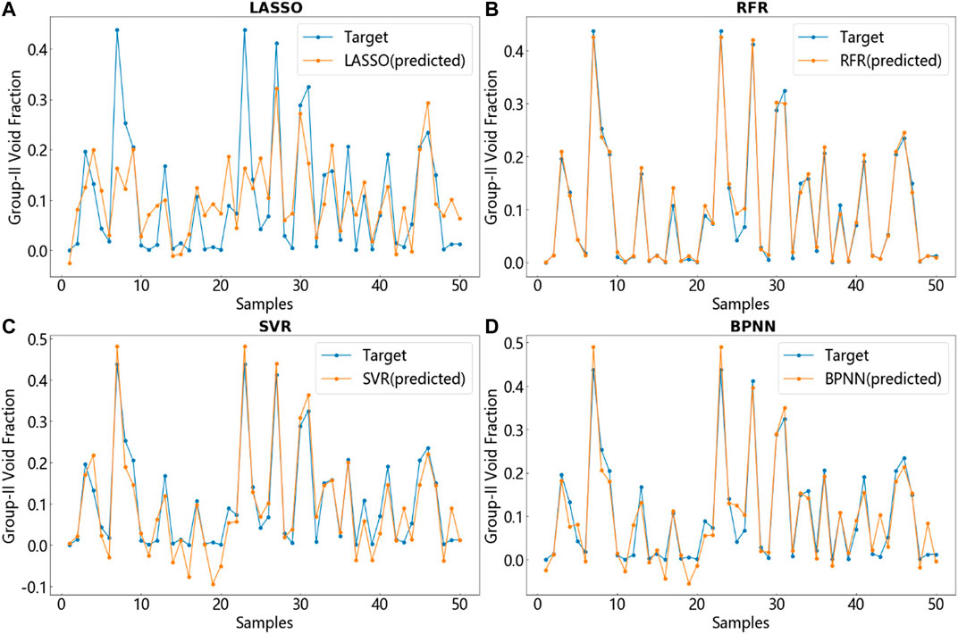
FIGURE 10. Prediction of the group-II void fraction using four models and comparison with target values. (A) LASSO. (B) RFR. (C) SVR (D) BPNN.

A phenomenon that can be clearly judged from the results shows that although each picture only takes 50 test set points (about $1/6$ of the total number of test sets) and the corresponding real values for visual display, a strong nonlinear characteristic is still showed by the real data set. It can be seen from Figures 7–10 that the predictive ability of LR is far inferior to the other three models. As a type of linear regression shipped with L1 regularization, one of the most crucial advantages of LR over non-linear models is LR usually performs great if the independent variables are linearly correlated with the dependent variable. However, non-linearity and scattered data features are obviously very disadvantageous and difficult for the LR algorithm because of its difficulty to capture the nonlinearity of dataset.

The performance of four models was measured by three metrics: ${\text{R}}^2$, $\text{RMSE}$ and $\text{CV}$ which are listed in Table 3. From the general distribution of the data, all models have significantly better predictive ability for group-I interfacial area concentration than group-II interfacial area concentration. Similarly, the predictive ability of all models for group-I void Fraction is significantly better than group-II void fraction. This phenomenon is consistent with the basic mechanism of two-phase flow, that is, the shape and size of the bubbles at the first interface are usually more regular and easier to predict than the bubbles at the second interface.

TABLE 3

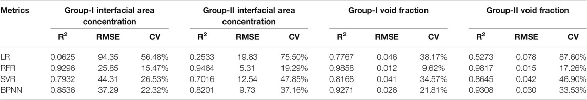
TABLE 3. The learning ability of the four models derived from the test set in terms of four two-phase flow parameter changes.

From the comparison of ${\text{R}}^2$ in Table 3, SVR and BPNN are significantly weaker than RFR in explaining experimental data in the present work. For the support vector regression, the prediction error $\text{CV}$ of the model for the four outputs is in the range of 26–48%, reflecting that there is still a certain gap between its prediction performance and actual experimental data. It is undeniable that the main advantages of SVR are that its computing power and complexity which do not depend on the dimensionality of the input space, its flexibility in dealing with nonlinear data, and its stability in dealing with slight changes in data (Awad and Khanna, 2015). However, one of the most prominent drawbacks of SVR is, for samples with discordant distributing complexities, the selection of reasonable parameters is very challenging (Liu et al., 2014), which is considered as the reason that SVR is not very satisfactory in terms of the data set fitting ability in the present research.

Finally, the two models RFR and BPNN are compared by using three metrics mentioned above. Although the interpretation of the data set by the two models is within an acceptable range, the prediction of the four outputs by RFR shows obviously higher accuracy rate. Although the neural network has a strong function approximation ability by preferentially fitting samples with higher discreteness in the data fitting process to achieve reduction in shavedness, but the learning ability of a single learner is always limited. By contrast, random forest, which belongs to ensemble learning, uses voting to solve the weak learning ability of a single learner and greatly improves the robustness of the model. For the prediction of the two sets of interfacial area concentrations, the errors of the RFR model are 15.47% and 19.49% while for the two sets of void fractions, the prediction errors of the RFR model are 9.62% and 17.26%. Moreover, it is worth mentioning that in the process of data preprocessing, the RFR requires simpler process, and the data required by its model does not need to be scaled. Because the numerical scaling does not affect the split point positions of the tree structure as well as the structure of the tree model. Moreover, the tree model cannot perform gradient descent because the tree model is constructed to find the best points by finding the optimal split points. Therefore, the tree model is stepped with non-differentiable step points, that means, the tree-structure model does not need to be normalized. In general, it is the distribution of the variables and the conditional probability between the variables instead of the values of the variables matter in tree-structure model. But for neural networks, the different feature ranges of the data will lead to catastrophic consequences such as gradient explosions. Consequently, the random forest regression algorithm shows robustness and effectiveness by taking advantage of the ‘wisdom of the crowds’ compared to other models in the present study. However, according to the mechanism of random forest regression in Section Random Forest Regression, the random forest regression model can only predict the data between the highest and lowest labels in the training data. For situations where the training and prediction inputs differ in their distributions, which named covariate shift (Tsuchiya et al., 2015), the characteristics of random forests that its disability to extrapolate will cause the attribute weights of its prediction outputs to be questionable. Therefore, it can be concluded that the explanatory and predictive capabilities of the random forest regression model for interfacial area concentration and void fraction in this study are better than those of the other three models, but whether the generalization ability of this model can be adapted to other working conditions still requires further exploration to verify. In addition, it is worth mentioning that, since the data used in this experiment is obtained from a rectangular channel of one size, this means that the size of the rectangular channel is not an input variable in this article. Therefore, it is unclear whether the generalization ability of the model obtained in this study can be applicable in rectangular channels of other sizes, which will be further explored in future research.

Conclusion

As an important cornerstone of artificial intelligence technology, machine learning has been widely used in many industries and various fields. The goal of this research is to explore the calculation of two-phase flow parameters based on data-driven methods in rectangular channels. In the paper, the four models, namely lasso regression, support vector machine regression, random forest regression and back propagation neural network regression were compared to mine and analyze the data collected through experiments, and the interfacial area concentration and void fraction were analyzed and predicted through the four models. It is found that the random forest regression is the most prominent algorithm among the four algorithms in terms of prediction accuracy, and meanwhile has strong anti-noise ability and good adaptability to nonlinear data. The prediction errors of four parameters including group-I interfacial area concentration, group-II interfacial area concentration, group-I void fraction and group-II void fraction predicted by the random forest regression are: 15.47, 19.29, 9.62 and 17.26%, respectively. In the future, data-driven methods are expected to be further applied in the prediction of other parameters of different flow conditions in rectangular channels, and the computational accuracy and efficiency of data-driven models could be improved further which shows the possibility of reducing the cost of experiment and replacing mechanical models in the nuclear reactor system safety analysis codes.

Data Availability Statement

The datasets presented in this article are not readily available because Due to the nature of this research, participants of this study did not agree for their data to be shared publicly, so supporting data is not available. Requests to access the datasets should be directed to huangqingyu950802@163.com.

Author Contributions

The authors confirm contribution to the paper as follows: study conception and design: QH and YY; data collection: YY; Data collation: QH, YY, and DC; Algorithms confirmation: QH; Implementation of Models: QH, YY, YZ, BP, and YZ; Analysis and interpretation of results: QH, YY, YZ, BP, and YW; Draft manuscript preparation: QH, YY, YZ, BP, and ZP. All authors reviewed the results and approved the final version of the manuscript.

Conflict of Interest

The authors declare that the research was conducted in the absence of any commercial or financial relationships that could be construed as a potential conflict of interest.

References

Awad, M., and Khanna, R. (2015). Efficient learning machines: theories, concepts, and applications for engineers and system designers. New York, NY: Springer Nature., 268.

Barre, F., and Bernard, M. (1990). The CATHARE code strategy and assessment. Nucl. Eng. Des. 124 (3), 257–284. doi:10.1016/0029-5493(90)90296-a

CrossRef Full Text | Google Scholar

Breiman, L. (1995). Better subset regression using the nonnegative garrote. Technometrics 37 (4), 373–384. doi:10.1080/00401706.1995.10484371

CrossRef Full Text | Google Scholar

Breiman, L. (2001a). Random forests. Mach. Learn. 45 (1), 5–32. doi:10.1023/a:1010933404324

CrossRef Full Text | Google Scholar

Breiman, L. (2001b). Statistical modeling: the two cultures (with comments and a rejoinder by the author). Stat. Sci. 16 (3), 199–231. doi:10.1214/ss/1009213726

CrossRef Full Text | Google Scholar

Gammerman, A. (1996). Machine learning: progress and prospects. London, UK: Royal Holloway.

Gomez-Fernandez, M., Higley, K., Tokuhiro, A., Welter, K., Wong, W. K., and Yang, H. (2020). Status of research and development of learning-based approaches in nuclear science and engineering: a review. Nucl. Eng. Des. 359, 110479. doi:10.1016/j.nucengdes.2019.110479

CrossRef Full Text | Google Scholar

Guo, L. J. (2002). Two-phase and multiphase flow dynamics. Xi’an, China: Xi’an Jiaotong University Press.

Guo, Z., and Uhrig, R. E. (1992). Use of artificial neural networks to analyze nuclear power plant performance. Nucl. Technol. 99 (1), 36–42. doi:10.13182/nt92-a34701

CrossRef Full Text | Google Scholar

Ishii, M., Kim, S., and Uhle, J. (2002). Interfacial area transport equation: model development and benchmark experiments. Int. J. Heat Mass Tran. 45 (15), 3111–3123. doi:10.1016/s0017-9310(02)00041-8

CrossRef Full Text | Google Scholar

Ishii, M. (1975). Thermo-fluid dynamic theory of two-phase flow. Paris, Eyrolles, Editeur., NASA Sti/recon Technical Report A 75, 29657.

Google Scholar

Kocamustafaogullari, G., and Ishii, M. (1995). Foundation of the interfacial area transport equation and its closure relations. Int. J. Heat Mass Tran. 38 (3), 481–493. doi:10.1016/0017-9310(94)00183-v

CrossRef Full Text | Google Scholar

Kohavi, R. (1995). A study of cross-validation and bootstrap for accuracy estimation and model selection. Ijcai 14 (2), 1137–1145.

Google Scholar

Kohonen, T. (1988). An introduction to neural computing. Neural Networks 1 (1), 3–16. doi:10.1016/0893-6080(88)90020-2

CrossRef Full Text | Google Scholar

Liu, Y., Jiang, B., Yi, H., and Bo, C. (2014). Fault isolation for nonlinear systems using flexible support vector regression. Math. Probl Eng. 2014, 1–10. doi:10.1155/2014/713018

CrossRef Full Text | Google Scholar

Lombardi, C., and Mazzola, A. (1997). Prediction of two-phase mixture density using artificial neural networks. Ann. Nucl. Energy 24 (17), 1373–1387. doi:10.1016/s0306-4549(97)00006-6

CrossRef Full Text | Google Scholar

Martin, R. P. (1995). RELAP5/MOD3 code coupling model. Nucl. Saf. 36 (2), 290–298.

Google Scholar

McClelland, J. L., and Rumelhart, D. E.PDP Research Group. (1986). Parallel distributed processing. Cambridge, MA: MIT press., Vol. 2, 20–21.

McLachlan, G. J., Do, K. A., and Ambroise, C. (2005). Analyzing microarray gene expression data. Hoboken, NJ: John Wiley & Sons.

Montes, J. L., Francois, J. L., Ortiz, J. J., Martín-del-Campo, C., and Perusquía, R. (2009). Local power peaking factor estimation in nuclear fuel by artificial neural networks. Ann. Nucl. Energy 36 (1), 121–130. doi:10.1016/j.anucene.2008.09.011

CrossRef Full Text | Google Scholar

Nair, V., and Hinton, G. E. (2010). “Rectified linear units improve restricted Boltzmann machines,” In Icml, Haifa, Israel, June 21–24, 2010.

Google Scholar

Radaideh, M. I., Pigg, C., Kozlowski, T., Deng, Y., and Qu, A. (2020). Neural-based time series forecasting of loss of coolant accidents in nuclear power plants. Expert Syst. Appl. 160, 113699. doi:10.1016/j.eswa.2020.113699

CrossRef Full Text | Google Scholar

Segal, M. R. (2004). Machine learning benchmarks and random forest regression. San Francisco, CA, Division of Biostatistics, University of California.

Su, G. H. (2013). Thermal-hydraulic calculation method for nuclear power system. Beijing, China: Tsinghua University Press.

Tambouratzis, T., and Pàzsit, I. (2010). A general regression artificial neural network for two-phase flow regime identification. Ann. Nucl. Energy 37 (5), 672–680. doi:10.1016/j.anucene.2010.02.004

CrossRef Full Text | Google Scholar

Tibshirani, R. (1996). Regression shrinkage and selection via the lasso. J. Roy. Stat. Soc. B. 58 (1), 267–288. doi:10.1111/j.2517-6161.1996.tb02080.x

CrossRef Full Text | Google Scholar

Tsuchiya, M., Yamauchi, Y., Yamashita, T., and Fujiyoshi, H. (2015). “Transfer forest based on covariate shift,” 2015 3rd IAPR asian conference on pattern recognition (ACPR), Kuala Lumpur, Malaysia, November 2015 (New York: IEEE.), 760–764.

Google Scholar

Van Rossum, G., and Drake, F. L. (1995). Python reference manual. Amsterdam: Centrum voor Wiskunde en Informatica.

Vapnik, V. (1998). “The support vector method of function estimation,” in Nonlinear modeling (Boston, MA: Springer.), 55–85.

CrossRef Full Text | Google Scholar

Zhang, G. Y., and Li, L. (2006). Support vector machine and its application research. Hunan: Hunan University.

Google Scholar