Short-Term Wind Power Forecasting Using Mixed Input Feature-Based Cascade-connected Artificial Neural Networks

Accurate short-term wind power forecasting is crucial for the efficient operation of power systems with high wind power penetration. Many forecasting approaches have been developed in the past to forecast short-term wind power. Artificial neural network-based approaches (ANNs) have become one of the most effective and popular short-term wind speed and wind power forecasting approaches in recent years. However, most researchers have used only historical data from a specific station to train the ANNs without considering meteorological variables from many neighboring stations on the forecasting performance. Using additional meteorological variables from neighboring stations can contribute valuable surrounding information to the forecasting model of the target station and improve ANNs performance. In this paper, a mixed input features-based cascade-connected artificial neural network (MIF-CANN) is used to train input features from many neighboring stations without encountering overfitting issues caused by many input features. Multiple ANNs train different combinations of input features in the first layer of the MIF-CANN model to produce preliminary results, then cascading into the second phase of the MIF-CANN model as inputs. The performance of the proposed MIF-CANN model is compared with the ANNs-based spatial correlation models. Simulation results show that the proposed MIF-CANN has better performance than the ANNs-based spatial correlation models.

Introduction

In recent years, conventional fossil fuels that have severe impacts on the global ecological systems have gradually been replaced by renewable energy (Chai et al., 2015). The wind is one of the most available, affordable, and efficient renewable sources. A total of 60.4 GW of wind power capacity was installed globally in 2019, a 19% increase from installations in 2018 (Global Wind Energy Council, 2020). However, power systems with high wind penetration will have to deal with many challenges, including real-time grid operations, competitive market designs, stability, and reliability of power systems (Soman et al., 2010). Accurate short-term wind power forecasting can be utilized to identify wind power fluctuations in advance to mitigate the impact of wind intermittency on the power system with high wind penetration (Soman et al., 2010; Peng et al., 2016).

In the literature, various wind power forecasting approaches have been proposed to improve the accuracy of short-term wind power forecasting (30 min to 6 h ahead). Most of the existing forecasting models (Wang et al., 2017; Hao and Tian., 2019; Sideratos and Hatziargyrious, 2007; Ren et al., 2016; Wu and Peng, 2017; Zameer et al., 2017; Liu et al., 2018) are using historical data from a specific target station without considering the effect of meteorological variables such as wind speed, wind direction, temperature, pressure and air density of the neighboring stations on the performance of forecasting model of the target station. Alexiadis et al. (1998) and Focken et al. (2002) found that the inclusion of meteorological variables from neighboring stations in the prediction model outperformed the models that only use the historical data of a single station. In Alexiadis et al. (1998); Ye et al. (2017), the authors used a mathematical equation-based spatial correlation method to learn the relationship between wind speeds at a target station and neighboring stations and utilized this relationship to enhance the forecasting model performance of the target station. However, the parameters of the mathematical equation-based spatial correlation models need to be tuned for each turbine, which is complicated and impractical (Ye et al., 2017). Instead of using complex mathematical equations to model the relationships among wind speeds at a target station and its neighboring stations, Alexiadis et al. (1998) and Zhu et al. (2018) have used ANNs to determine the relationships. Alexiadis et al. (1999) used a feedforward-ANN model to determine the wind speed relationship between a target station and neighboring stations. Zhu et al. (2018) used a predictive deep convolutional neural network as a spatial correlation model to learn the wind speed relationships of different stations.

However, most of the existing machine learning spatial correlation models have only used variables from a few neighboring stations (i.e., less than 5) (Alexiadis et al., 1999; Zhu et al., 2018). Furthermore, the majority of the existing spatial correlation models have used only wind speed from neighboring stations as inputs, other meteorological variables such as wind direction, temperature, atmospheric pressure, and air density are seldomly considered (Alexiadis et al., 1998; Alexiadis et al., 1999; Ye et al., 2017; Zhu et al., 2018). It has been shown in (Chen and Folly, 2019) that meteorological variables from neighboring stations such as wind direction, temperature, and atmospheric pressure can also affect the target station’s wind speed forecasting. Target station is the station where wind power forecasting is required. Therefore, it is essential to include meteorological variables as input variables into the target station’s forecasting model. Zhou et al. (2017) and Chen and Folly (2020) have used multiple meteorological variables to measure the spatial correlation between two stations to enhance the spatial correlation model’s prediction performance. However, the number of neighboring stations involved in (Zhou et al., 2017) and (Chen and Folly, 2020) was relatively small (i.e., less than 5). Although using meteorological variables from many neighboring stations (i.e., larger than 25 stations) could allow the forecasting model to better learn the spatial characteristic of wind speed and provide better forecasting results, it is challenging. One of the disadvantages of using many neighboring stations’ meteorological variables to train ANN-based models is model overfitting (Li et al., 2015). ANNs might over-fit the model or not recognize patterns from the input data with many input variables (Wimmer and Powell, 2016). Therefore, a model that can both take a large number of inputs and avoid model overfitting issues is proposed.

In this paper, a mixed input features-based cascade-connected artificial neural network (MIF-CANN), consisting of 30 first layer predictors and a single second layer predictor, is used to obtain input features from 30 neighboring stations. For example the first predictor only takes inputs from the target station. The second predictor takes inputs from the target station and a neighboring station. The third predictor takes input from the target station and two neighboring stations. Preliminary outputs of all 30 predictors were cascaded to the second layer of the proposed model as inputs, which the second layer predictor then trains to produce a final output. In this way, the proposed MIF-CANN model was able to obtain meteorological information from many neighboring stations and avoid overfitting.

The main contributions of this paper are as follows. The impact of various meteorological variables from many neighboring stations on the performance of ANN-based forecasting models is evaluated. A mixed input features-based cascade-connected artificial neural network is proposed to effectively learn useful information of a large number of input features and at the same time avoid model overfitting issues. More advanced forecasting models can apply the same model structure as the proposed model to minimize overfitting issues.

The rest of this paper is organized as follows. Training Data briefly introduces data collection, data preprocessing, and input-output pairs for supervised learning. Artificial Neural Networks Based Spatial Correlation describes the configuration selection of an ANN model, the building block of the proposed model, and explains the ANN-based spatial correlation model structure. The Proposed Mixed input feature-Based Cascade-Connected Artificial Neural Network Model presents the construction steps of the MIF-CANN Model. Simulation Results and Discussions discuss the evaluation metrics and simulation results of short-term wind speed and wind power forecasting. Finally, the findings of the paper are summarized in the Conclusion section.

Training Data

Date Collection

The acronyms used in this paper are shown in Table 1. The flowchart of the methodology is shown in Figure 1. As shown in Figure 1, the first step is collecting and preprocessing the data. The second step is to determine a suitable basic ANN model configuration which is shown in Artificial Neural Networks . The third step is to construct both the ANN-based spatial correlation model and the proposed MIF-CANN. Data used in this paper were collected from the National Renewable Energy Laboratory (NREL). The NREL datasets consist of wind power, wind speed, wind direction, temperature, barometric pressure, air density. NREL’s wind power data are generated from the Weather Research and Forecasting (WRF) model version 3.4.1. Table 2 summarizes the variables’ descriptive statistics from the NREL: ID61118 dataset (Wind Prospector, 2019). In our opinion, the quality of the dataset used in this study is good because it does not contain any missing values and outliers. The quality of the meteorological variables and wind power of the NREL datasets is also validated by NREL (King, Clifton, and Hodge, 2014; Draxl et al., 2015). The ten minutely data of each station from January 2007 to October 2009 (150,000 samples) are used for the model training and validation. Data from April 2011 to October 2012 (75,000 samples) are used for model testing.

TABLE 1

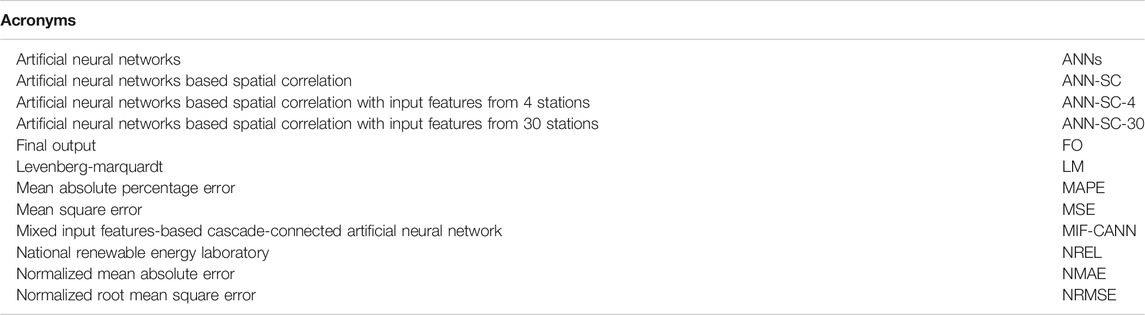
TABLE 1. Summary of acronyms used in this paper.

FIGURE 1

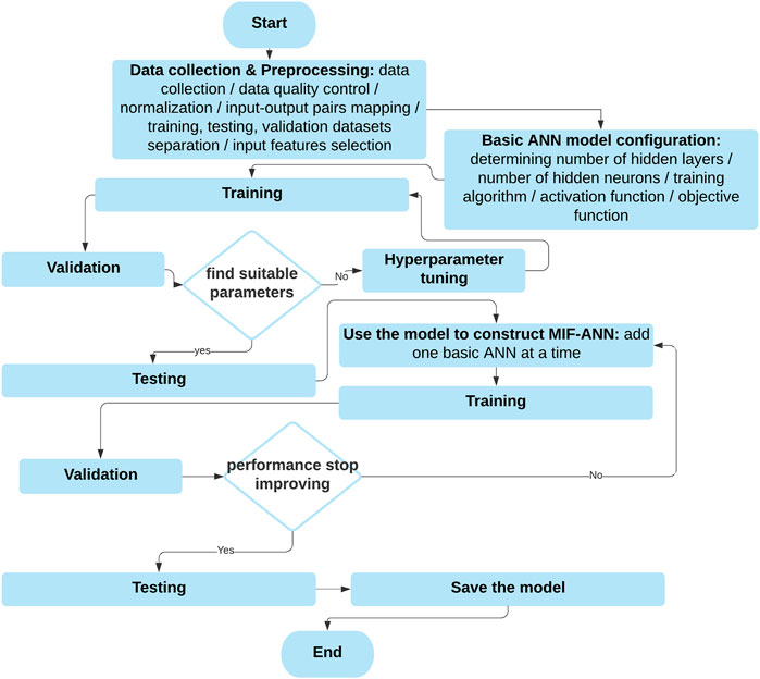
FIGURE 1. Flowchart of the methodology.

TABLE 2

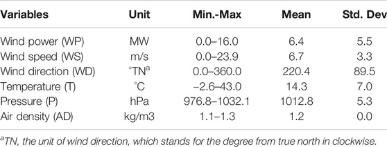
TABLE 2. Summary of the descriptive statistics of the NREL: ID61118 dataset.

Normalization

Variables with larger values might suppress the impact of the one with smaller values on the forecasting model. The normalization technique minimizes the impact by scaling the values of different input variables into the same range (usually from 0 to 1 or from -1 to 1) to improve the model convergence rate and forecasting accuracy.

Linear mapping over a specified range is the most commonly used normalization method. A minimum-maximum normalization technique, which is defined as Equation 1, is used in this paper.

$X_i^{\text{'}}=\left(\frac{X_i-X_{min}}{X_{max}-X_{min}}\right)\left(X_{max}^{\text{'}}- X_{min}^{\text{'}}\right)+ X_{min}^{\text{'}}(1)$

where $X_i$, $X_{min}$, $X_{max}$ , $X_i^{\text{'}}$, $X_{min}^{\text{'}}$, $X_{max}^{\text{'}}$, is the mean, minimum, and maximum of the actual input data and the corresponding normalized values, respectively. In this paper, $X_{min}^{\text{'}}$ is set to 0 and $X_{max}^{\text{'}}$, is set to 1 to match the range of the logistic sigmoid function of ANNs.

Input-Output Pairs for Supervised Learning

The time interval between samples denotes forecast interval (data resolution), and the forecasting horizon is the length of time into the future for which forecasts are to be prepared. This paper focuses on short-term wind speed and wind power forecasting ranging from 30 min to 6 h ahead (Soman et al., 2010; Chang, 2014; Jung and Broadwater, 2014). The data resolution of the NREL dataset is 10 min per sample. For example, for two hours ahead forecasting, the gap between input and output samples is 12 steps (12 × 10 min = 120 min = 2 h). Table 3 shows input-output pairs for ANN models. As can be seen, all five of the meteorological variables shown in Table 2 were used as inputs and wind speed as the output. The sample gap between inputs and the output is 12 steps which are represented by using t-12. Other than meteorological variables, time of day [time indicator (TI)] is also used as an input because it contains a cyclic characteristic. Therefore, it is essential to label the input data with time of day so the forecasting models can recognize the daily cycle within the wind speed time series. The range of time indicator (TI) is between 1 and 144 (cover 24 h of a day)

TABLE 3

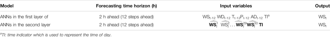
TABLE 3. Input-output pairs for ANN model.

Artificial Neural Networks Based Spatial Correlation

Artificial Neural Networks

A simple but efficient feedforward-ANN with two hidden layers, each containing ten hidden neurons, was used by Chen and Folly (2019) to effectively handle the complicated relationship between wind speed and other meteorological variables such as wind direction, temperature, temperature gradient, pressure and relative humidity. The number of hidden layers and hidden neurons were selected using the rule-of-thumb and trial and error approach (Karsoliya, 2012). Different combinations of hidden layers and hidden neurons were tested. The best performer was chosen for the final model configuration. Examples of some varieties of numbers of hidden layers and hidden neurons that have been considered in this article are listed in Table 4. The simulation results indicate that a feedforward-ANN with two hidden layers, each contain ten hidden neurons, was adequate for the short-term wind power forecasting. As a result, the feedforward-ANN with two hidden layers, each with ten hidden neurons, was used in this study as the core structure of the ANN-SC model and the first-layer predictors of the proposed MIF-CANN model. As can be seen in Figure 2, the feed-forward ANN contains two hidden layers, and each hidden layer contains n hidden neurons. The relationship between the inputs and output of each node is defined as (Tesfaye et al., 2016):

$Y_i=f_i({\displaystyle \sum }_{j=1}^n{W}_{ij}.X_j+b_i)(2)$

where X_j is the j^th input, Y_i is the output, W^ij is the connection weight, b_i is the bias, and f_i is the activation function.

TABLE 4

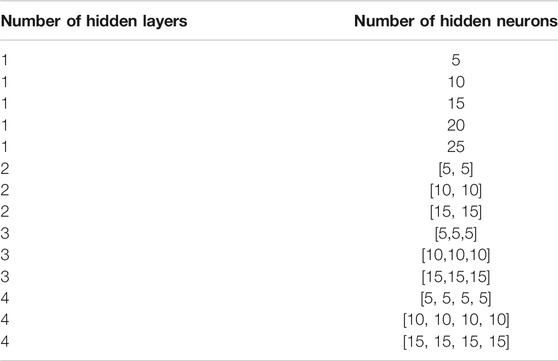
TABLE 4. Some combinations of different numbers of hidden layers and hidden neurons tested in this research.

FIGURE 2

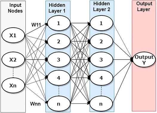
FIGURE 2. Structure of a feed-forward ANN model with two hidden layers each contains ten hidden neurons.

The next step was to find a suitable training algorithm. The back-propagation algorithm is one of the most commonly used algorithms for ANNs. Levenberg-Marquardt (LM) is a popular training algorithm. It is the combination of the Gauss-Newton method and the steepest descent method. LM is defined as:

$X_{K+1}=X_K-{\left[J^{T}J+\mu I\right]}^{-1}{J}^{T}e(3)$

where x is the training weight, $\mu$ is the damping factor, J is the Jacobian matrix of the first derivatives of the network errors with respect to the weights and biases, I is the identity matrix, and e is a vector of network errors. Thus, when $\mu$is zero, LM becomes Newton’s method. On the other hand, when $\mu$is large, LM becomes gradient descent with a small step size (MathWorks, 2019). As a result, LM has the speed advantage of the Gauss-Newton method and the stability advantage of the steepest descent method. Therefore, Levenberg-Marquardt back-propagation algorithm was utilized in this study.

Artificial neural networks use activation functions to map the relationship between input data and output targets (Santos and Da Silva 2014). The logistic sigmoid function, a nonlinear function, was used in this paper’s hidden layer to capture the nonlinear relationship between inputs and outputs. The range of normalized variables is also from 0 to 1. The logistic sigmoid function is defined as:

$f\left(x\right)=\frac{1}{\left(1+e^{-x}\right)}(4)$

A linear activation function was used to return the weighted sum of the input in the output layer. The initial weights and biases of the ANNs are generated randomly. The minimization of the mean square error (MSE) between the input data such as wind speed, wind direction, temperature, pressure, air density, time indicator, and the target data, wind speed of the target station, is the objective function.

Artificial Neural Networks-Based Spatial Correlation

In this paper, station ID61118 from the NREL datasets was used as the target station due to its central location. The surrounding stations of Station ID61118 were used as the neighboring stations. It has been shown in (Chen and Folly, 2019) that all the available meteorological variables have different levels of impact on the short-term wind speed and wind power forecasting performance. Therefore, all the meteorological variables shown in Table 2 were used as inputs in this study. The selection of neighboring stations was mainly based on two criteria. The first one was based on the wind speed correlation coefficient between the target and neighboring stations. The second one was based on the stations’ geographical location. Spearman rank correlation is preferred to describe the monotonic nonlinear relationship between two variables (Schober, Boer, and Schwarte, 2018). Wind speed frequency distribution graphs of different stations were different, some of them were similar to the normal distribution curve, and some were not. Therefore, the Spearman rank correlation determines the wind speed correlation between two stations in this paper. The neighboring stations with high wind speed correlation with the target station and low wind speed correlation with the selected neighboring stations were added to the ANN-SC model.

Spearman rank correlation is defined as Equation 5 (Mukaka, 2012):

${\rho }_s\left(x, y\right)=1- \frac{6{{\displaystyle \sum }}_{i=1}^N\left(d_i\right)2}{N(N^2-1)}(5)$

where $d_i$ is the difference between the ranks of the ith variables; N is the total number of observations.

In our previous work (Chen and Folly, 2020), we used an ANN-based spatial correlation model to forecast short-term wind power. It was suggested that the ANN-based spatial correlation model’s forecasting performance could be further improved if meteorological variables from more neighboring stations were used as inputs. However, it was found that the model’s performance improved up to a certain number (i.e. 15) of neighboring station before started to deteriorate, as we will show later. Figure 3 shows the structure of the forecasting model of the ANN-SC used. As can be seen in Figure 3, meteorological variables from 30 stations were used. That is, input features from a target station and 29 neighboring stations were considered. Meteorological variables from neighboring stations allow the ANN-SC model to learn the upwind and downwind information to enhance forecasting performance. The ANN-SC model used in this paper is similar to the one used in (Chen and Folly, 2020), except that more meteorological variables are used in this paper. In (Chen and Folly, 2020), the ANN-SC model used meteorological variables from four stations (herein called ANN-SC-4), whereas in this paper, meteorological variables from 30 (herein called ANN-SC-30) are used.

FIGURE 3

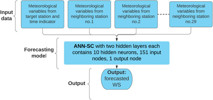
FIGURE 3. Structure of the ANN-SC with the input features from 1 target station and 29 neighboring stations.

The Proposed Mixed Input Features-Based Cascade-Connected Artificial Neural Network Model

Although the ANN-SC model can utilize the information provided by the meteorological variables of neighboring stations to enhance forecasting performance, the ANN-SC model can only handle a limited number of input features. A large number of input features might over-fit ANNs. Therefore, the proposed MIF-CANN model uses 30 feed-forward ANNs, each with two hidden layers as the first-layer predictors, and a feed-forward ANN with a single hidden layer at the second layer to mitigate the overfitting effect arising from using the ANN-SC model.

The parallel structure of the MIF-CANN model mimics the structure of ANNs, which allows its second layer ANN to assign weights to the stronger predictors to mitigate the chance of overfitting. Due to the space limitation, only a portion of the MIF-CANN model’s structure is shown in Figure 4 as an example. As shown in Figure 4, the first-layer nodes indicate the input features sources, i.e., input features from the target station are indicated as T1, and input features from the first neighboring station are indicated as N1. Thus, P1 to P6 are used to identify the predictors of the MIF-CANN model. P1 means that the predictor uses input features from one station, whereas P6 means that the predictor uses input features from six stations (i.e., one target station and five neighboring stations).

FIGURE 4

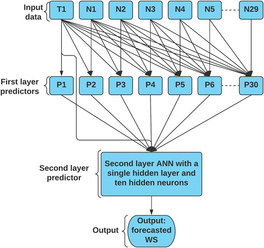
FIGURE 4. The structure of the proposed MIF-CANN model with input features from one target station and the structure of the proposed MIF-CANN model neighboring stations.

Figure 5 shows the flowchart of the proposed MIF-CANN training process, which used two main steps to obtain a final forecasting result. The first step was to get preliminary outputs from each of the 30 predictors (i.e., P1 to P30). The output of each predictor was obtained by using Equation 6.

$Y_i=f{\displaystyle \sum }_{h2=1}^{10}f\left[{\displaystyle \sum }_{h1=1}^{10}W({\displaystyle \sum }_{j=1}^i\left(X_j\right)+TI)+b\right] (6)$

where Y_i is the output of the i^th predictor; f is the activation function; W is the connection weight; X_j is the meteorological variables from i stations, TI is the time indicator, b is the bias. In the second step, the outputs of 30 first layer predictors were cascaded into the second layer as inputs, which were trained by the second layer ANN to obtain the final results. The second layer ANN nonlinearly assigned bigger weights to the outputs of the stronger first layer predictors and smaller weights to the outputs of the weaker predictors. The final output (FO) of MIF-CANN was obtained by using Equation 7.

$FO=f({\displaystyle \sum }_{i=1}^{30}W.Y_i+b)(7)$

where f is the activation function; W is the connection weight; Y_i is the preliminary output of the i^th predictor; b is the bias.

FIGURE 5

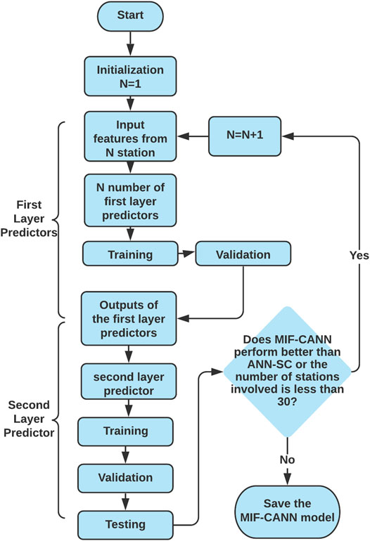
FIGURE 5. Flowchart of the proposed MIF-CANN model.

The proposed MIF-CANN model can obtain meteorological information from a large number of neighboring stations. Simultaneously, it can select only useful information to enhance forecasting performance and mitigate the overfitting problem of large models.

Simulation Results and Discussions

All the simulations were run in MATLAB R2020a on a computer with an Intel(R) Xeon (R) E-2104G CPU @ 3.20 GHz and 16 GB of RAM. Forecasting time horizons of all the simulation results presented for this study were 2 hours ahead forecasting.

Three of the most commonly used forecasting evaluation metrics (i.e., NRMSE, NMAE, MAPE) were applied for this study to evaluate the proposed models’ forecasting performance. Normalized root mean square error (NRMSE) is more sensitive to large errors when compared to normalized mean absolute error (NMAE) because the errors are squared before they are averaged (Wesner, 2016; Uniejewski, Marcjasz, and Weron, 2019). Mean absolute percentage error (MAPE) is preferred when the forecast error cost has a higher correlation with the percentage error than the numerical size error (Azadeh et al., 2011). NRMSE, NMAE equations can be found in (Chen and Folly, 2019). MAPE is defined as:

$MAPE=\frac{100}{N}{\displaystyle \sum }_{t=1}^N\left|\frac{e_t}{\overline{P}}\right|(8)$

$\overline{P}= \frac{1}{N}{\displaystyle \sum }_{t=1}^N{P}_t(9)$

where$e_t$ the is the forecasting error of sample t, N is the total number of samples, $P_t$ is wind speed or wind power in this paper.

The summary of the model structure and training time of the three forecasting models is shown in Table 5. As shown in Table 5, the ANN-SC-4 model and ANN-SC-30 model have a more straightforward model structure than the proposed MIF-CANN model. However, a longer time is required to train the more complex MIF-CANN model.

TABLE 5

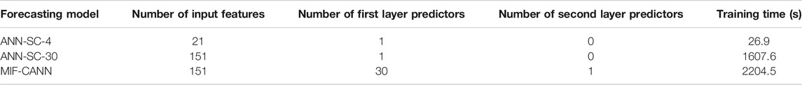
TABLE 5. Summary of the model structure and training time of three forecasting models.

Short-Term Wind Speed Forecasting

The simulation results of 2 h-ahead wind speed forecasting of three forecasting approaches are shown in Table 6. The ANN-SC-4 proposed in (Chen and Folly, 2020) used input features from one target station and three neighboring stations. Both the ANN-SC-30 model and the MIF-CANN model used input features from a total of 30 stations. As shown in Table 6, the proposed MIF-CANN model has the best short-term wind speed forecasting performance, followed by the ANN-SC-30 model. The forecasting performance of the MIF-CANN model and the ANN-SC-30 model improved by 25.35% and 6.62% with respect to the ANN-SC-4 model, respectively. This result suggests that additional input features from more neighboring stations can enhance the ANN-based model. The significant improvement of the MIF-CANN model compared to the ANN-SC-30 model indicates that the model with mixed input features and cascaded structure can further enhance the forecasting performance of the ANNs-based spatial correlation model (ANN-SC). Figure 6 shows the training time of ANN-SC and MIF-CANN against the number of stations involved. As can be seen from Figure 6, both the proposed model and ANN-SC take longer to train with a larger number of input features.

TABLE 6

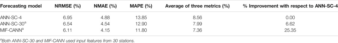
TABLE 6. Simulation results of 2 h-ahead wind speed forecasting of the three forecasting approaches.

FIGURE 6

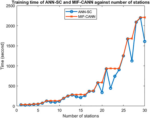
FIGURE 6. The training time of ANN-SC and MIF-CANN against the number of stations.

The NRMSE, NMAE, and MAPE values of 2 h-ahead wind speed forecasting of the ANN-SC model (i.e., from ANN-SC-1 to ANN-SC-30) and the MIF-CANN model are shown in Table 7. The simulation results of every 5^th additional station are shown in Table 7 to shorten the tables’ length. As shown in Table 7, there is an advantage in using the MIF-CAN model over the ANN-SC model when the number of neighboring stations involved becomes larger than 15. The average value of three evaluation metrics of the MIF-CANN model with input features from 30 stations improved by 7.97% compared to the ANN-SC-30 model.

TABLE 7

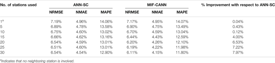
TABLE 7. Simulation results of 2 h-ahead wind speed forecasting of the ANN-SC and MIF-CANN.

Figure 7 shows the evaluation results of the ANN-SC and the MIF-CANN models against the number of stations used to train the forecasting models. The downward trend of all the evaluation metrics suggests that the neighboring stations’ input features do have a positive impact on the forecasting performance of the target station. However, when the number of neighboring stations involved in the ANN-SC model training become too large (i.e., more than 25 stations), the improvement in the target station’s forecasting performance stopped. This is due to the model overfitting caused by using many input features from the neighboring stations.

FIGURE 7

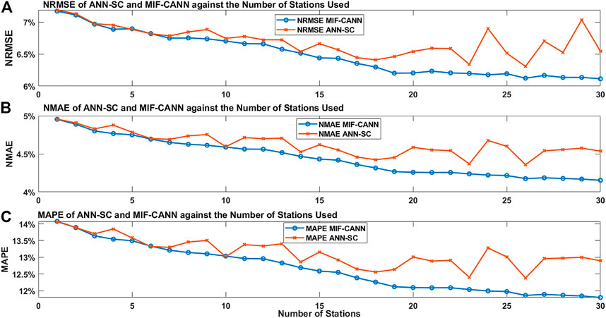
FIGURE 7. The evaluation results of the ANN-SC and MIF-CANN against input features from different numbers of stations: (A), NRMSE, (B), NMAE, (C), MAPE.

The advantage of using MIF-CANN is not very obvious when a small number of neighboring stations (i.e., less than 15) is used in the forecasting model training. However, both the ANN-SC and the MIF-CANN can handle a small number of input features. Although additional meteorological variables from neighboring stations can enhance the forecasting model’s performance, using too many input features can overfit the forecasting model. The proposed MIF-CANN model performs better than the ANN-SC model when the number of neighboring stations used for training becomes larger than 15 stations. The first layer predictors of the MIF-CANN model with different input features produce relatively diverse outputs. The MIF-CANN model used a second layer ANN model to train the outputs of the first layer predictors. Thus, using a total of 30 outputs which contain useful information from 30 first layer predictors as input features to train the second layer predictors can provide useful information from 151 input features and at the same time avoid over-fitting issue.

Although the MIF-CANN is more complicated than the ANN-SC-30 model, the parallel structure of the MIF-CANN model allows all 30 predictors to be trained simultaneously. Therefore, the MIF-CANN model’s training time is equal to the sum of the longest training time of its first layer predictors and the training time of the second layer model. The MIF-CANN model requires a slightly longer training time than the ANN-SC-30 model. Both forecasting models were trained offline, and forecasting accuracy is a more critical performance measuring factor than the training time. As a result, the MIF-CANN is preferred over the ANN-SC-30 model for short-term wind power forecasting.

Short-Term Wind Power Forecasting

The forecasted wind speed was converted to wind power. The benefit of using the MIF-CANN model is verified by comparing its forecasting performance to the ANN-SC-4 model and the ANN-SC-30 model. The simulation results of 2 h-ahead wind power forecasting of the three models are shown in Table 8. As can be seen in Table 8, the MIF-CANN model performs better than the two ANN-SC models. The average value of the three evaluation metrics of the MIF-CANN model improved by 8.51% and 15.12% compared to the ANN-SC-30 model and the ANN-SC-4 model, respectively. The performance of the three models was evaluated by checking the error histogram. Figure 8 shows the forecasting error histograms of ANN-SC-4, ANN-SC-30, and MIF-CANN. As shown in Figure 8, most forecasting errors (indicated in red) of MIF-CANN are concentrated near the Zero Error line. Therefore, the red color is much less than the green or blue color on the sides of the graph.

TABLE 8

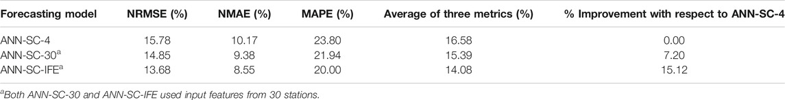
TABLE 8. Simulation results of 2 h-ahead wind power forecasting of the three forecasting approaches.

FIGURE 8

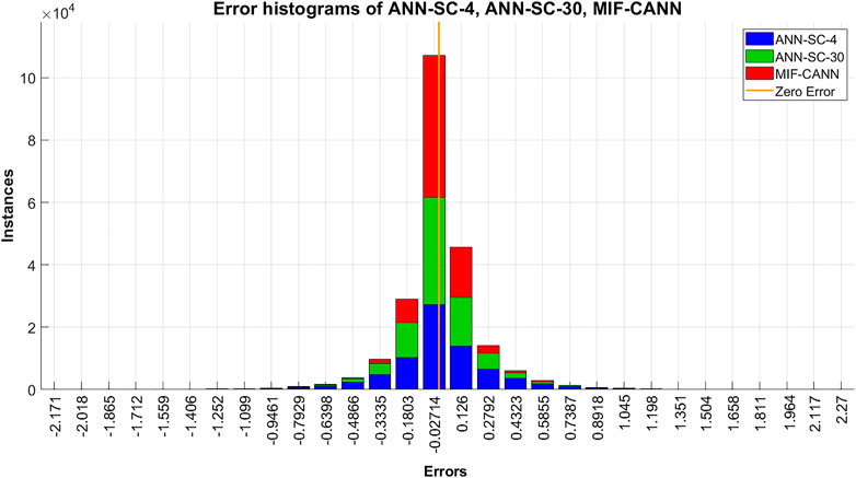
FIGURE 8. Error histograms of ANN-SC-4, ANN-SC-30, MIF-CANN.

Figure 9 shows the simulated wind power and the forecasted wind power of the ANN-SC-4 model, the ANN-SC-30 model, the MIF-CANN model. As shown in Figure 9, the two hours ahead forecasted wind power of all three models could closely track the simulated power. The forecasting error of the MIF-CANN model is smaller than that of the ANN-SC-4 model and the ANN-SC-30 model for the peaks and downward regions (i.e., between hour 1 and hour 3; between hour 12 and hour 15). The results suggest that the MIF-CANN model can take additional information from many neighboring stations to provide the best results. Therefore, both spatial correlation and cascaded structure can be used together to handle several input features and avoid overfitting issues. Figure 10 shows the 95% forecasting confidence interval of the proposed MIF-CANN. As shown in Figure 10, the forecasted wind power can track the simulated wind power closely for most of the samples. The 95% prediction confidence interval covers most of the simulated wind power except hour 8 and hour 20 which is due to the unexpected sudden changes in wind speed. Wind ramp events need to be considered in further studies to improve the forecasting performance further.

FIGURE 9

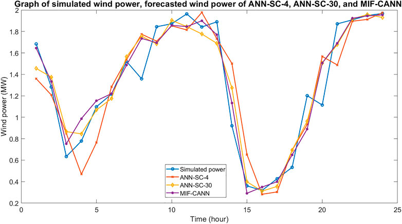
FIGURE 9. Graph of simulated wind power and forecasted wind power of the ANN-SC-4 model, the ANN-SC-30 model, and the MIF-CANN model.

FIGURE 10

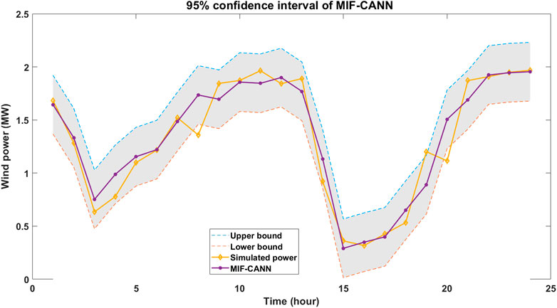
FIGURE 10. 95% forecasting confidence interval of the proposed MIF-CANN.

Conclusion

In this paper, a mixed input features-based cascade-connected artificial neural network (MIF-CANN) was used to enhance the short-term wind speed and wind power forecasting performance of ANN-based spatial correlation (ANN-SC) models. The ANN-SC model improved the forecasting performance by using meteorological variables such as wind speed, wind direction, temperature, pressure and air density from neighboring stations compared to the case where a small amount or none of the meteorological variables from neighboring stations were used. However, the ANN-SC model's performance deteriorates when the input features are too large (i.e., input features from more than 25 neighboring stations). The proposed MIF-CANN model utilized 30 feed-forward ANNs in the first layer to obtain surrounding meteorological information from many neighboring stations. It then employed a second layer ANN model to train the outputs of 30 first-layer ANN predictors to enhance the forecasting performance. Although the structure of the proposed MIF-CANN is much larger than ANN-SC, it mimics the parallel structure of ANN, which can train input features in parallel. Therefore, the training time of MIF-CANN is very similar to ANN-SC. The simulation results indicate that the proposed MIF-CANN model can obtain useful information from many input features without encountering the model overfitting issues. Thus, the spatial correlation and cascaded techniques can be applied together to more advanced artificial intelligence-based models to enhance short-term wind speed and wind power forecasting performance.

Data Availability Statement

Publicly available datasets were analyzed in this study. This data can be found here (NREL WIND PROSPECTOR) (https://maps.nrel.gov/wind-prospector/).

Author Contributions

QC was responsible for the concept, methodology, simulations, and the initial draft of the paper; KAF supervised the paper and provided input on the research concept and methodology and the final draft of the paper.

Funding

This research was funded in part by the National Research Foundation (NRF) of South Africa, grants number NRF Grant UID 118550.

Conflict of Interest

The authors declare that the research was conducted in the absence of any commercial or financial relationships that could be construed as a potential conflict of interest.

Publisher’s Note

All claims expressed in this article are solely those of the authors and do not necessarily represent those of their affiliated organizations, or those of the publisher, the editors and the reviewers. Any product that may be evaluated in this article, or claim that may be made by its manufacturer, is not guaranteed or endorsed by the publisher.

Acknowledgments

The financial assistance of the National Research Foundation (NRF) towards this research is hereby acknowledged. This research is partially supported financially in part by the NRF. Opinions expressed and conclusions arrived at, are those of the author and are not necessarily to be attributed to the NRF.

References

Alexiadis, M. C., Dokopoulos, P. S., Sahsamanoglou, H. S., and Manousaridis, I. M. (1998). Short-term Forecasting of Wind Speed and Related Electrical Power. Solar Energy 63 (1), 61–68. doi:10.1016/S0038-092X(98)00032-2

CrossRef Full Text | Google Scholar

Alexiadis, M. C., Dokopoulos, P. S., and Sahsamanoglou, H. S. (1999). Wind Speed and Power Forecasting Based on Spatial Correlation Models. IEEE Trans. Energy Convers. 14 (3), 836–842. doi:10.1109/60.790962

CrossRef Full Text | Google Scholar

Azadeh, A., Sheikhalishahi, M., Tabesh, M., and Negahban, A. (2011). The Effects of Preprocessing Methods on Forecasting Improvement of Artificial Neural Networks. Aust. J. Basic Appl. Sci. 5 (6), 570–580.

Google Scholar

Chai, S., Xu, Z., Lai, L. L., and Wong, K. P. (2015). “An Overview on Wind Power Forecasting Methods,” in International Conference on Machine Learning and Cybernetics. Guangzhou. IEEE, 765–770. doi:10.1109/ICMLC.2015.7340651

CrossRef Full Text | Google Scholar

Chang, W.-Y. (2014). A Literature Review of Wind Forecasting Methods. Jpee 02, 161–168. doi:10.4236/jpee.2014.24023

CrossRef Full Text | Google Scholar

Chen, Q., and Folly, K. (2019). “Effect of Input Features on the Performance of the ANN-Based Wind Power Forecasting,” in 2019 SAUPEC/RobMech/PRASA Conference. Bloemfontein. IEEE, 673–678. doi:10.1109/RoboMech.2019.8704725

CrossRef Full Text | Google Scholar

Chen, Q., and Folly, K. (2020). “Short-term Wind Power Forecasting Based on Spatial Correlation and Artificial Neural Network,” in Southern African Universities Power Engineering Conference/ Robotics and Mechatronics/ Pattern Recognition Association of South Africa. Cape Town. IEEE. doi:10.1109/SAUPEC/RobMech/PRASA48453.2020.9041033

CrossRef Full Text | Google Scholar

Draxl, C., Hodge, B. M., Clifton, A., and McCaa, J. (2015). Overview and Meteorological Validation of the Wind Integration National Dataset Toolkit. Denver: National Renewable Energy Laboratory (NREL). doi:10.2172/1214985

CrossRef Full Text

Focken, U., Lange, M., Mönnich, K., Waldl, H.-P., Beyer, H. G., and Luig, A. (2002). Short-term Prediction of the Aggregated Power Output of Wind Farms-A Statistical Analysis of the Reduction of the Prediction Error by Spatial Smoothing Effects. J. Wind Eng. Ind. Aerodynamics 90, 231–246. doi:10.1016/S0167-6105(01)00222-7

CrossRef Full Text | Google Scholar

Global Wind Energy Council (2020). Global Wind Energy Council. Available at: https://gwec.net/gwec-over-60gw-of-wind-energy-capacity-installed-in-2019-the-second-biggest-year-in-history/.

Google Scholar

Hao, Y., and Tian, C. (2019). A Novel Two-Stage Forecasting Model Based on Error Factor and Ensemble Method for Multi-step Wind Power Forecasting. Appl. Energ. 238, 368–383. doi:10.1016/j.apenergy.2019.01.063

CrossRef Full Text | Google Scholar

WesnerJ. (2016). Human in a Machine World March. Available at: https://medium.com/human-in-a-machine-world/mae-and-rmse-which-metric-is-better-e60ac3bde13d (Accessed August 31, 2019).

Jung, J., and Broadwater, R. P. (2014). Current Status and Future Advances for Wind Speed and Power Forecasting. Renew. Sust. Energ. Rev. 31, 762–777. doi:10.1016/j.rser.2013.12.054

CrossRef Full Text | Google Scholar

Karsoliya, S. (2012). Approximating Number of Hidden Layer Neurons in Multiple Hidden Layer BPNN Architecture. Int. J. Engine. Trends Technol. 3, 714–717.

King, J., Clifton, A., and Hodge, B. M. (2014). Validation of Power Output for the WIND Toolkit. Denver: National Renewable Energy Laboratory. doi:10.2172/1159354

CrossRef Full Text

Li, S., Wang, P., and Goel, L. (2015). Wind Power Forecasting Using Neural Network Ensembles with Feature Selection. IEEE Trans. Sustain. Energ. 6 (4), 1447–1456. doi:10.1109/TSTE.2015.2441747

CrossRef Full Text | Google Scholar

Liu, H., Duan, Z., Li, Y., and Lu, H. (2018). A Novel Ensemble Model of Different Mother Wavelets for Wind Speed Multi-step Forecasting. Appl. Energ. 228, 1783–1800. doi:10.1016/j.apenergy.2018.07.050

CrossRef Full Text | Google Scholar

MathWorks, (2019). "MathWorks," The Matchworks, Inc., [Online]. Available at: https://www.mathworks.com/help/deeplearning/ref/trainlm.html. (Accessed October 22, 2019).

Google Scholar

Mukaka, M. M. (2012). Statistics Corner: A Guide to Appropriate Use of Correlation Coefficient in Medical Research. Malawi Med. J. 24 (3), 69–71.

PubMed AbstractGoogle Scholar

Peng, X., Deng, D., Wen, J., Xiong, L., Feng, S., and Wang, B. (2016). “A Very Short Term Wind Power Forecasting Approach Based on Numerical Weather Prediction and Error Correction Method,” in International Conference on Electricity Distribution. Xi'an. IEEE. doi:10.1109/CICED.2016.7576362

CrossRef Full Text | Google Scholar

Ren, Y., Suganthan, P. N., and Srikanth, N. (2016). A Novel Empirical Mode Decomposition with Support Vector Regression for Wind Speed Forecasting. IEEE Trans. Neural Netw. Learn. Syst. 27 (8), 1793–1798. doi:10.1109/TNNLS.2014.2351391

PubMed Abstract | CrossRef Full Text | Google Scholar

Santos, C. A. G., and Da Silva, G. B. L. (2014). Daily Streamflow Forecasting Using a Wavelet Transform and Artificial Neural Network Hybrid Models. Hydrological Sci. J. 59 (2), 2150–3435. doi:10.1080/02626667.2013.800944

CrossRef Full Text | Google Scholar

Schober, P., Boer, C., and Schwarte, L. A. (2018). Correlation Coefficients. Anesth. Analgesia 126 (5), 1763–1768. doi:10.1213/ANE.0000000000002864

PubMed Abstract | CrossRef Full Text | Google Scholar

Sideratos, G., and Hatziargyriou, N. D. (2007). An Advanced Statistical Method for Wind Power Forecasting. IEEE Trans. Power Syst. 22 (1), 258–265. doi:10.1109/TPWRS.2006.889078

CrossRef Full Text | Google Scholar

Soman, S. S., Zareipour, H., Malik, O., and Mandal, P. (2010). “A Review of Wind Power and Wind Speed Forecasting Methods with Different Time Horizons,” in IEEE. North American Power Symposium. Arlington, TX, USA. IEEE, 1–8. doi:10.1109/NAPS.2010.5619586

CrossRef Full Text | Google Scholar

Tesfaye, A., Zhang, J. H., Zheng, D. H., and Shiferaw, D. (2016). Short-term Wind Power Forecasting Using Artificial Neural Networks for Resource Scheduling in Microgrids. Ijsea 5 (3), 144–151. doi:10.7753/ijsea0503.1005

CrossRef Full Text | Google Scholar

Uniejewski, B., Marcjasz, G., and Weron, R. (2019). Understanding Intraday Electricity Markets: Variable Selection and Very Short-Term price Forecasting Using LASSO. Int. J. Forecast. 35, 1533–1547. doi:10.1016/j.ijforecast.2019.02.001

CrossRef Full Text | Google Scholar

Wang, H.-z., Li, G.-q., Wang, G.-b., Peng, J.-c., Jiang, H., Jiang, H., et al. (2017). Deep Learning Based Ensemble Approach for Probabilistic Wind Power Forecasting. Appl. Energ. 188, 56–70. doi:10.1016/j.apenergy.2016.11.111

CrossRef Full Text | Google Scholar

Wimmer, H., and Powell, L. (2016). “Principle Component Analysis for Feature Reduction and Data Preprocessing in Data Science,” in Proceedings of the Conference on Information Systems Applied Research. Vegas, Nevada: Las Vegas.

Google Scholar

Wind Prospector (2019). National Renewable Energy Laboratory. Available at: https://maps.nrel.gov/wind-prospector/ (Accessed November 11, 2019).

Google Scholar

Wu, W., and Peng, M. (2017). A Data Mining Approach Combining $K$ -Means Clustering with Bagging Neural Network for Short-Term Wind Power Forecasting. IEEE Internet Things J. 4 (4), 979–986. doi:10.1109/JIOT.2017.2677578

CrossRef Full Text | Google Scholar

Ye, L., Zhao, Y., Zeng, C., and Zhang, C. (2017). Short-term Wind Power Prediction Based on Spatial Model. Renew. Energ. 101, 1067–1074. doi:10.1016/j.renene.2016.09.069

CrossRef Full Text | Google Scholar

Zameer, A., Arshad, J., Khan, A., and Raja, M. A. Z. (2017). Intelligent and Robust Prediction of Short Term Wind Power Using Genetic Programming Based Ensemble of Neural Networks. Energ. Convers. Manage. 134, 361–372. doi:10.1016/j.enconman.2016.12.032

CrossRef Full Text | Google Scholar

Zhou, H., Xue, Y., Guo, J., and Chen, J. (2017). Ultra-short-term Wind Speed Forecasting Method Based on Spatial and Temporal Correlation Models. J. Eng. (Iet) 2017 (13), 1071–1075. doi:10.1049/joe.2017.0494

CrossRef Full Text | Google Scholar

Zhu, Q., Chen, J., Zhu, L., Duan, X., and Liu, Y. (2018). Wind Speed Prediction with Spatio-Temporal Correlation: a Deep Learning Approach. Energies 11 (4). doi:10.3390/en11040705

CrossRef Full Text | Google Scholar